The active bijection for graphs

Abstract

The active bijection forms a package of results studied by the authors in a series of papers in oriented matroids. The present paper is intended to state the main results in the particular case, and more widespread language, of graphs. We associate any directed graph, defined on a linearly ordered set of edges, with one particular of its spanning trees, which we call its active spanning tree. For any graph on a linearly ordered set of edges, this yields a surjective mapping from orientations onto spanning trees, which preserves activities (for orientations in the sense of Las Vergnas, for spanning trees in the sense of Tutte), as well as some partitions (or filtrations) of the edge set associated with orientations and spanning trees. It yields a canonical bijection between classes of orientations and spanning trees, as well as a refined bijection between all orientations and edge subsets, containing various noticeable bijections, for instance: between orientations in which smallest edges of cycles and cocycles have a fixed orientation and spanning trees; or between acyclic orientations and no-broken-circuit subsets. Several constructions of independent interest are involved. The basic case concerns bipolar orientations, which are in bijection with their fully optimal spanning trees, as proved in a previous paper, and as computed in a companion paper. We give a canonical decomposition of a directed graph on a linearly ordered set of edges into acyclic/cyclic bipolar directed graphs. Considering all orientations of a graph, we obtain an expression of the Tutte polynomial in terms of products of beta invariants of minors, a remarkable partition of the set of orientations into activity classes, and a simple expression of the Tutte polynomial using four orientation activity parameters. We derive a similar decomposition theorem for spanning trees. We also provide a general deletion/contraction framework for these bijections and relatives.

 

1 Introduction

The general setting of this paper is to relate orientations and spanning trees of graphs, and to study graphs on a linearly ordered set of edges, in terms of structural properties, fundamental constructions, decompositions, enumerative properties, and bijections. The original motivation was to provide a bijective interpretation and a structural understanding of the equality of two classical expressions of the Tutte polynomial, one in terms of spanning tree activities by Tutte [43]:

$\displaystyle t(G;x,y)=\sum_{\iota,\varepsilon}t_{\iota,\varepsilon}x^{\iota}y^{\varepsilon}$

where $t_{\iota,\varepsilon}$ is the number of spanning trees of the graph $G$ with internal activity $\iota$ and external activity $\varepsilon$, the other in terms of orientation activities by Las Vergnas [38]:

$\displaystyle t(G;x,y)=\sum_{\iota,\varepsilon}o_{\iota,\varepsilon}\ \Bigl{(}{x\over 2}\Bigr{)}^{\iota}\ \Bigl{(}{y\over 2}\Bigr{)}^{\varepsilon}$

where $o_{\iota,\varepsilon}$ is the number of orientations of $G$ with dual-activity $\iota$ and activity $\varepsilon$, which contains various famous enumerative results from the literature, such as counting acyclic reorientations (and more generally regions in hyperplane arrangements and oriented matroids), e.g. [46, 42, 47, 32].

Our solution is made of several constructions and results of independent interest, whose central achievement is to associate, in a canonical way, any directed graph ${\overrightarrow{G}}$ defined on a linearly ordered set of edges with one particular of its spanning trees, denoted $\alpha({\overrightarrow{G}})$, which we call the active spanning tree of ${\overrightarrow{G}}$. For any graph on a linearly ordered set of edges, this yields a surjective mapping from orientations onto spanning trees, which preserves the above activities, and such that exactly $2^{\iota+\varepsilon}$ orientations with orientation activities $(\iota,\varepsilon)$ are associated with the same spanning tree with spanning tree activities $(\iota,\varepsilon)$. This yields a canonical bijection between remarkable orientation classes and spanning trees (depending only on the ordered undirected graph), along with a naturally refined bijection between orientations and edge-subsets (depending in addition on any fixed reference orientation).

Before turning into the graph language, let us give to the reader one of the shortest possible complete definition of the active basis in the general setting of oriented matroids. For any oriented matroid $M$ on a linearly ordered set $E$, the active basis $\alpha(M)$ of $M$ is determined by:

• Fully optimal basis of a bounded region. If $M$ is acyclic and every positive cocircuit of $M$ contains $\mathrm{min}(E)$, then $\alpha(M)$ is the unique basis $B$ of $M$ such that:

  • for all $b\in B\setminus p$, the signs of $b$ and $\mathrm{min}(C^{*}(B;b))$ are opposite in $C^{*}(B;b)$;

  • for all $e\in E\setminus B$, the signs of $e$ and $\mathrm{min}(C(B;e))$ are opposite in $C(B;e)$.

• Duality. $\alpha(M)=E\setminus\alpha(M^{*}).$

• Decomposition. $\alpha(M)=\alpha(M/F)\ \uplus\ \alpha(M(F))$ where $F$ is the union of all positive circuits of $M$ whose smallest element is the greatest possible smallest element of a positive circuit of $M$.

This definition, developed in [14, 24, 25, 26], applies to directed graphs: for a directed graph ${\overrightarrow{G}}$ on a linearly ordered set of edges $E$, we have $\alpha({\overrightarrow{G}})=\alpha(M({\overrightarrow{G}}))$ where $M({\overrightarrow{G}})$ is the usual oriented matroid on $E$ associated with ${\overrightarrow{G}}$. In Section 4 of the present paper, we directly define $\alpha({\overrightarrow{G}})$ in terms of graphs. However, a specificity of graphs is their lack of duality, which implies that the definitions have to be adapted. Throughout the paper, in comparison with [24, 25, 26], the fact that a graph does not have a dual graph forces us to repeat some definitions and some proofs, first from the primal viewpoint and second from the dual viewpoint, which is usually a simple translation using cycle/cocycle duality, whereas, in (oriented) matroids, definitions and proofs can be shortened by applying them directly to the dual. Other specificities of the graph case will be mentioned later.

What we call the active bijection is actually a three-level construction, summarized in the diagram of Figure 1. It is based on several results of independent interest, including various Tutte polynomial expressions as shown in this diagram, yielding various bijections listed in Table 1, and forming a consistent whole. Let us describe all this along with the organization of the paper. In what follows, $G$ is a graph on a linearly ordered set of edges, also called ordered graph for short.

Figure 1: Diagram of results and constructions for the active bijection of an ordered graph $G$. Horizontal arrows indicate in which ways the constructions or definitions apply (the deletion/contraction constructions can be used to build the whole bijections as matchings rather than mappings). Vertical arrows indicate how objects are related. Dotted rectangles indicate how the Tutte polynomial is involved or transforms through the constructions. All results quoted in the diagram are proved in terms of graphs in the paper (or the companion paper [29]), except Theorem 5.50 [26] and Theorem 4.29 [20, 24] (alternative or more general proofs of all results can be found in [24, 25, 26, 27, 28]).

orientations	spanning trees/subsets
canonical active bijection of an ordered undirected graph
activity classes of orientations	spanning trees	$t(G;1,1)$
activity classes of acyclic orientations	internal spanning trees	$t(G;1,0)$
activity classes of strongly connected orientations	external spanning trees	$t(G;0,1)$
bipolar orientations (up to opposite)	uniactive internal spanning trees	$t_{1,0}$
cyclic-bipolar orientations (up to opposite)	uniactive external spanning trees	$t_{0,1}$
refined active bijection w.r.t. a given reference orientation
orientations	subsets of the edge set	$t(G;2,2)$
orientations with fixed orientation for active edges	forests	$t(G;2,1)$
orientations with fixed orientation for dual-active edges	connected spanning subgraphs	$t(G;1,2)$
acyclic orientations	no-broken-circuit subsets	$t(G;2,0)$
strongly connected orientations	supersets of external spanning trees	$t(G;0,2)$
orientations with fixed orientation            for active edges and dual-active edges	spanning trees	$t(G;1,1)$
acyclic orientations with            fixed orientation for dual-active edges	internal spanning trees	$t(G;1,0)$
strongly connected orientations with            fixed orientation for active edges	external spanning trees	$t(G;0,1)$
particular cases
(for suitable orderings) unique sink acyclic orientations	internal spanning trees	[20, Section 6]
(complete graph seen as a chordal graph) permutations	increasing trees	[21, Section 5]

Table 1: Active bijections and noticeable restrictions. The first blocks of lines come from Theorems 4.34 and 4.41. The third column indicates the evaluation (or the coefficient) of the Tutte polynomial that counts the involved objects. Activity classes of orientations are obtained by arbitrarily reorienting parts of the active partition/filtration (see Section 3), that is by arbitrarily reorienting unions of all directed cycles or cocycles whose smallest edges are greater than a given edge. Internal, resp. external, spanning trees are those whose external activity, internal activity equals 0, and they are uniactive when the other activity equals 1 (see Section 2.2). Active/dual-active edges of an ordered directed graph are smallest edges of directed cycles/cocycles (see Section 2.3). An orientation is said to have fixed orientation for some edge it this edge has the same direction as in a given reference orientation of the graph (see Section 3.3). The two last lines recall particular cases addressed in other papers.

At the first level, the uniactive bijection of $G$ concerns the case where $\iota=1$ and $\varepsilon=0$ in the above setting, hence the term uniactive, which includes also the case where $\iota=0$ and $\varepsilon=1$ by some dual construction. This case is addressed for graphs in [20, 29] (see [24, 27] in oriented matroids, or [26, Section 5] for a summary). Let us sum it up below. Details are recalled in Section 4.1.

In [20] (see also [24]), we showed that a bipolar directed graph ${\overrightarrow{G}}$ on a linearly ordered set of edges, with adjacent unique source and sink connected by the smallest edge, has a unique so-called fully optimal spanning tree $\alpha({\overrightarrow{G}})$ that satisfies a simple criterion on fundamental cycle/cocycle directions (let us point out that this is a tricky theoretical result, with various interpretations, see the summary [26, Section 5] for details and [29] for complexity issues). Associating bipolar orientations of $G$ (with fixed orientation for the smallest edge) with their fully optimal spanning trees provides a canonical bijection with spanning trees with internal activity 1 and external activity 0 (called uniactive internal). It is a classical result from [47], also implied by [38], that those two sets have the same size, also known as the $\beta$ invariant of the graph [8], that is $\beta(G)=t_{1,0}=(1/2).o_{1,0}$.

In the companion paper [29], we address the problem of computing the fully optimal spanning tree. The inverse mapping, producing a bipolar orientation for which a given spanning tree is fully optimal, is very easy to compute by a single pass over the ordered set of edges. But the direct computation is complicated and it had not been addressed in previous papers. When generalized to real hyperplane arrangements, the problem contains and strengthens the real linear programming problem (as shown in [24], hence the name fully optimal). This “one way function” feature is a noteworthy aspect of the active bijection. In general, we give a direct construction by means of elaborations on linear programming [23, 27], allowing for a polynomial time computation. This construction is translated and adapted in the graph case in the companion paper [29].

Finally, from [20, Section 4] (see also [24, Section 5] or [26, Section 5]), the bijection between bipolar orientations and their fully optimal spanning trees directly yields a bijection between orientations obtained from bipolar orientations by reversing the source-sink edge, namely cyclic-bipolar orientations, and spanning trees with internal activity $0$ and external activity $1$. This framework involves a remarkable duality property, the so-called active duality, essentially meaning that those two bijections are related to each other consistently with cycle/cocycle duality (that is oriented matroid duality, which extends planar graph duality, see Section 4.1). Let us mention that this duality property can be also seen as a strengthening of linear programming duality (see [24, Section 5]), and that it is also related to the equivalence of two dual formulations in the deletion/contraction construction of the uniactive bijection (see Section 6.1 or the companion paper [29]).

At the second level, which is the central achievement of the whole construction and of this paper, we define the active spanning tree $\alpha({\overrightarrow{G}})$ of an ordered directed graph ${\overrightarrow{G}}$, from the previous bipolar and cyclic-bipolar cases, by means of some decompositions of orientations and spanning trees. Then, the canonical active bijection is the bijection between preimages and images of the surjective mapping ${\overrightarrow{G}}\mapsto\alpha({\overrightarrow{G}})$, from orientations of $G$ to spanning trees of $G$, where preimages are characterized as natural equivalence classes in terms of the above decomposition of orientations, called activity classes. In other words, it is the combination of the uniactive bijection and those two decompositions for orientations and spanning trees. It is called canonical because it is built from those three independent canonical constructions, and because it is an intrinsic attribute of the undirected ordered graph $G$ (depending on the ordering but not depending on any orientation of $G$). These constructions have been shortly defined without proofs in [20]. The definition and properties of the canonical active bijection are addressed in Section 4.2. The decomposition of orientations and its various implications is addressed in Section 3 (those results are generalized to oriented matroids in [26]). The decomposition of spanning trees is briefly addressed in Section 5, obtained as corollaries of the previous results (see below). Now, let us precise the section contents.

In Section 3.1, we define the active partition/filtration of the set of edges of an ordered directed graph, a notion already introduced in [20] (see [26] for a geometrical interpretation in oriented matroids, and [15] for a generalization to oriented matroid perspectives and hence, in a sense, to directed graph homomorphisms). We show how to decompose a directed graph on a linearly ordered set of edges into a sequence of minors that are either bipolar or cyclic-bipolar. This construction refines the usual partition of the edge set into the union of directed cycles (yielding a strongly connected minor) and the union of directed cocycles (yielding an acyclic minor). We mention that the notion of active partition turns out to generalize a notion of vertex partition which is relevant in [7, 45, 13, 35], see Remark 3.5 for more information and [20, Section 7] for details.

In Section 3.2, considering all orientations of a graph, and building on a uniqueness property in the previous decomposition, we derive a general decomposition theorem for the set of all orientations, in terms of particular sequences of 2-connected minors (Theorem 3.14). The involved sequences of subsets provide a remarkable notion of filtrations for ordered graphs. Enumeratively, this decomposition can be seen as an expression of the Tutte polynomial in terms of products of beta invariants of minors (Theorem 3.15). This formula refines at the same time the formulas in terms of spanning tree activities [43], of orientation activities [38], and the convolution formula [11, 33]. Actually, it can be also seen as the enumerative interpretation of a spanning tree decomposition, see below (and in this context, it is generalized to matroids in [25]).

In Section 3.3, we define activity classes of orientations, obtained by reversing independently all parts in the active partition/filtration. Activity classes are isomorphic to boolean lattices and form a remarkable partition of the set of orientations. We show how this directly yields a simple expression of the Tutte polynomial using four orientation activity parameters (Theorem 3.24), as announced in [40]. This expression is the counterpart for orientations of a similar four parameter formula for subsets/supersets of spanning trees [31, 41] (Theorem 2.2). Furthermore, in each activity class, there is one and only one representative orientation with fixed direction for smallest edges of directed cycles or cocycles. In particular, as shown in [20, Section 6], given a vertex and a suitable ordering of the edge set (when all branches of the smallest spanning tree are increasing from the vertex), there is one and only one acyclic orientation with this vertex as a unique sink in each activity class of acyclic orientations. This discussion is continued in Section 4.3 about the refined active bijection, which relates the two above four parameter Tutte polynomial expressions.

In Section 4.2, we define the active spanning tree as explained above, by gluing together the images, by the uniactive bijection of Section 4.1, of the bipolar and cyclic-bipolar minors of the decomposition of Section 3. Equivalently, this definition can be formulated in a recursive way, as in the beginning of this introduction. This yields a canonical bijection between activity classes of orientations and spanning trees (Theorem 4.34), as shown in Table 1. Furthermore, this bijection not only preserves activities and active edges, but also active partitions that one can also define for spanning trees, as explained below.

Section 5 has a special status in the paper, as it addresses the constructions from the spanning tree viewpoint, whereas the rest of the paper is focused on the orientation viewpoint. First, in Section 5.1, we state counterparts in terms of spanning trees of the aforementioned decomposition of orientations. The main result is a decomposition theorem for spanning trees of an ordered graph in terms of the same filtrations, or the same particular sequences of minors, as above, into spanning trees with internal/external activities equal to $1/0$ or $0/1$ (Theorem 5.43). It refines the decomposition into two internal/external parts from [11]. As far as proofs are concerned, in this paper, we essentially prove this spanning tree decomposition in Section 4.2, at the same time as the canonical active bijection properties, building on the decomposition of orientations. It could also be defined and proved independently of the rest of constructions, directly in terms of spanning trees (which is the approach used in [25] to define these decompositions in matroids). Here we take advantage of the fact that graphs are orientable (in contrast with matroids: such proofs using orientations are not possible in non-orientable matroids).

Second, in Section 5.2, we give reformulations of the definitions of the active bijection starting from spanning trees, and we give a simple construction building, for a given spanning tree, at the same time the active partition of this spanning tree and its preimage under the canonical active bijection. It consists in a single pass over the set of edges and uses only fundamental cycles and cocycles. This section is given for completeness of the paper, but it is proved in [25, 26] (in contrast with the rest of the paper which is self-contained). Actually, it is the combination of a single pass construction of the active partition of (the fundamental graph of) a matroid basis [25], and the single pass inverse construction for the uniactive bijection alluded to above and recalled in Section 4.1. This construction also readily applies to the refined active bijection (the third level of the active bijection addressed below). The simplicity of the construction from spanning trees to orientations is again a noteworthy aspect of the active bijection.

At the third level of the active bijection, in Section 4.3, we choose a reference orientation ${\overrightarrow{G}}$ of $G$, and we define the refined active bijection of $G$ w.r.t. ${\overrightarrow{G}}$, denoted $\alpha_{\overrightarrow{G}}$, which is a mapping from $2^{E}$ to $2^{E}$. Precisely, it applies to $A\subseteq E$, by:

$\alpha_{\overrightarrow{G}}(A)=\alpha(-_{A}{\overrightarrow{G}})\ \setminus\ \bigl{(}A\cap O^{*}(-_{A}{\overrightarrow{G}})\bigr{)}\ \cup\ \bigl{(}A\cap O(-_{A}{\overrightarrow{G}})\bigr{)},$

where $O(-_{A}{\overrightarrow{G}})$, resp. $O^{*}(-_{A}{\overrightarrow{G}})$, denotes the set of smallest edges of a directed cycle, resp. cocycle, of $-_{A}{\overrightarrow{G}}$. This mapping provides a bijection between all subsets of edges $A\subseteq E$, thought of as orientations $-_{A}{\overrightarrow{G}}$, and all subsets of edges, thought of as subsets/supersets of spanning trees (Theorem 4.40), along with various interesting restrictions as shown in Table 1. In particular, $\alpha_{\overrightarrow{G}}(A)$ equals the spanning tree $\alpha(-_{A}{\overrightarrow{G}})$ when $A$ does not meet $O^{*}(-_{A}{\overrightarrow{G}})$ nor $O(-_{A}{\overrightarrow{G}})$, that is when the directions of smallest edges of directed cycles and cocycles agree with their directions in the reference orientation ${\overrightarrow{G}}$, which yields a bijection between spanning trees and these representatives of activity classes. This natural refinement of the canonical active bijection has been briefly introduced in [14, 22] and we develop it into the details. The construction is the following. The canonical active bijection maps an activity class of orientations onto a spanning tree. On one hand, the activity class is isomorphic to a boolean lattice, and activity classes partition the set of orientations. On the other hand, each spanning tree $T$ is associated with a classical subset interval $[T\setminus\mathrm{Int}(T),T\cup\mathrm{Ext}(T)]$, where $Int(T)$, resp. $Ext(T)$, denotes the set of internally, resp. externally, active edges of $T$ [9] (see also [10, 30, 41] for generalizations). These intervals are also isomorphic to boolean lattices, and partition the power set of $E$. The canonical active bijection can be seen as associating each activity class to an isomorphic spanning tree interval. Then the choice of a reference orientations ${\overrightarrow{G}}$ allows for breaking the symmetry in the two boolean lattices and specifying a boolean lattice isomorphism for each such couple. By this way, this refined active bijection preserves the four refined activity parameters alluded to above for orientations and for subsets about Section 3.3.

Let us point out that the constructions used at the three levels of the active bijection are fundamentally independent of each other. As explained in Section 4.4, one can get a whole large class of activity preserving bijections following the same decomposition framework: start at the first level with any arbitrary bijection between bipolar orientations and uniactive spanning trees, extend it at the second level using the same recursive definition, and set arbitrary boolean lattice isomorphisms at the third level. The active bijection is obtained by a canonical choice at each level.

In Section 6, we complete the paper by providing deletion/contraction constructions of the above active bijections: the uniactive one (Theorem 6.52, extract from the companion paper [29] which addresses the problem of computing the fully optimal spanning tree of an ordered bipolar digraph), the canonical one (Theorem 6.58), and the refined one (Theorem 6.63). We point out that those deletion/contraction constructions provide a global approach: they can be used to build the whole bijections at once, as a matching between orientations and spanning trees, rather than as a mapping (see Remark 6.60, see also [29, Remark LABEL:ABG2LP-rk:ind-10] in terms of complexity). We also present a general deletion/contraction framework for building correspondences/bijections between orientations and spanning trees/edge subsets involving more or less constraining activity preservation properties. Here again, the active bijection is determined by canonical choices.

At the end, in Section 7, we completely analyze the example of $K_{3}$ and $K_{4}$ (much more illustrations and details on the same example can be found in [25, 26]).

Further notes on the scope of this paper

This paper is intended for a reader primarily interested in graph theory. It is essentially self-contained and written in the graph language. Meanwhile, it is inspired from oriented matroid theory, meaning for example that the technique and constructions do not use the vertices of the graph at all, and often manipulates or highlights minors, combinations of cycles/cocycles, as well as cycle/cocycle duality.

Beyond graphs, this work is the subject of several papers by the present authors [19, 20, 21, 22, 23, 24, 25, 26, 27, 28]. In a much more general context, the active bijection has a geometrical flavour, in real hyperplane arrangements or pseudosphere arrangements. The main papers, which provide the whole construction in oriented matroids, are [24, 25, 26, 27, 28], and the reader can see the introduction of [26] for a more general and detailed overview. The previous paper on graphs [20] was a graphical version of [24]. Now, roughly, as mentioned in the above introduction, the present paper condenses the papers [25, 26, 28] and adapts them in terms of graphs (the main results of [25], available in matroids, are derived here from graph orientability), and the companion paper [29] condenses and adapts [27]. More examples, figures, results and details, which apply in particular to graphs, can be found in these papers [24, 25, 26, 27, 28]. Summaries can be found in [22, 17] (and a survey had been given in [18], partial translation of [14] in english and obsolete as for today).

Let us also highlight [21] which addresses the case of chordal graphs, also called triangulated graphs, in the more general context of supersolvable hyperplane arrangement (see [21, Example 3.2]). In particular, for acyclic orientations of the complete graph with a suitable edge set ordering, the active bijection coincides with a well-known bijection between permutations and increasing trees (see [21, Section 5] for details and references).

Originally, the question of relating spanning tree and orientation activities came from a paper by the second author [38], following on from which, in [39], a definition for a correspondence between spanning trees and orientations of graphs was proposed. It was based on an algorithm, given without a proof, which inspired the decomposition of activities developed for the active bijection, but which does not yield the correspondence given by the active bijection (not for general activities, nor for the restriction to $1/0$ activities, and nor with respect to duality). Also, let us mention that a different notion of activities for graph orientations had been introduced even earlier in [3], along with incorrect constructions according to [38]. Finally, the active bijection has been introduced in the Ph.D. thesis of the first author [14], where most of the results from [19, 20, 21, 22, 23, 24, 25, 26, 27, 28] were given, at least in a preliminary form.

Further literature notes

Information on literature related to specific results of the paper is given throughout the paper. To end this introduction, let us give further references on results involving orientations and spanning trees in graphs, distinct from the active bijection.

The equality between the number of unique sink acyclic orientations and internal spanning trees comes from [47]. A bijection between these objects appeared in [12], and our more involved bijection [20, Section 6] (see also Theorem 4.40) answers a question in this paper [12, (a) p. 145].

According to our knowledge, the first bijection between acyclic orientations and no-broken-circuit subsets in graph appeared in [6]. Another bijection between orientations and no-broken-circuit subsets appeared in [2] in the context of parking functions.

Other bijections between acyclic orientations, resp. strongly connected orientations, resp. general orientations, and internal-type, resp. external-type spanning trees, resp. edge subsets appeared in [4]. They rely on a different notion of activities, for spanning trees only, and depending on rotation schemes of combinatorial maps instead of linear orderings of the edge set.

However, none of the above bijections [12, 6, 4, 2] is intended to preserve activities, and none of them seems to generalize to hyperplane arrangements nor to oriented matroids.

Lastly, let us mention the recent work [1] which gathers both subset activity parameters (addressed in Section 2.5) and orientation activity parameters (addressed in Section 3.3) in a large Tutte polynomial expansion formula in the context of graph fourientations. This work also extends to graph fourientations a deletion/contraction property addressed in Section 6.4, see Remark 6.65.

2 Preliminaries

2.1 Generalities

For the sake of simple exposition, graphs in this paper are usually assumed to be connected, but the results apply to non-connected graphs as well, up to direct adaptations such as replacing spanning trees with spanning forests. Graphs can have loops and multiple edges. The 2-connectivity of a graph means its 2-vertex connectivity, and we consider a loopless graph on two vertices with at least one edge as 2-connected. Loops and isthmuses have the ususal meaning. A graph can be called loop, or isthmus, if it has a unique edge and this unique edge is a loop, or not a loop, respectively. A digraph is a directed graph, and an ordered graph is a graph $G=(V,E)$ on a linearly ordered set of edges $E$. Edges of a directed graph are supposed to be directed or equally oriented. A directed graph will be denoted with an arrow, ${\overrightarrow{G}}$, and the underlying undirected graph without arrow, $G$. Reversing the directions of a subset of edges $A$ in a directed graph ${\overrightarrow{G}}$ is called reorienting, and the resulting directed graph is denoted $-_{A}{\overrightarrow{G}}$. The digraph obtained by reorienting all edges is called the opposite digraph. The cycles, cocycles, and spanning trees of a graph $G=(V,E)$ are considered as subsets of $E$, hence their edges can be called their elements. The cycles and cocycles of $G$ are always understood as being minimal for inclusion. Given $F\subseteq E$, we denote $G(F)$ the graph obtained by restricting the edge set of $G$ to $F$, that is the minor $G\setminus(E\setminus F)$ of $G$ (observe that $G(F)$ is not necessarily connected, isolated vertices are pointless and can be ignored). For $e\in E$, a minor $G/\{e\}$, resp. a minor $G\backslash\{e\}$, resp. a subset $A\backslash\{e\}$ for $A\subseteq E$, can be denoted for short $G/e$, resp. $G\backslash e$, resp. $A\backslash e$. If $\mathcal{F}$ is a set of subsets of $E$, then $\cup\mathcal{F}$ denotes the subset of $E$ obtained by taking the union of all elements of $\mathcal{F}$. In the paper, $\subset$ denotes the strict inclusion, and $\uplus$ (or $+$) denotes the disjoint union. We call correspondence when several objects (e.g. some orientations) are associated with the same object (e.g. a spanning tree) by a surjection (hence a bijection can be seen as a one-to-one correspondence).

2.2 Spanning tree activities

Let $G$ be an ordered (connected) graph and let $T$ be a spanning tree of $G$. The next definitions are almost not practically used in the rest of the paper, but we use them here to define the Tutte polynomial and to settle the general setting of the paper. For $b\in T$, the fundamental cocycle of $b$ with respect to $T$, denoted $C_{G}^{*}(T;b)$, or $C^{*}(T;b)$ for short, is the cocycle joining the two connected components of $T\setminus\{b\}$. Equivalently, it is the unique cocycle contained in $(E\setminus T)\cup\{b\}$. For $e\not\in T$, the fundamental cycle of $e$ with respect to $T$, denoted $C_{G}(T;e)$, or $C(T;e)$ for short, is the unique cycle contained in $T\cup\{e\}$. Let

$$\mathrm{Int}(T)=\Bigl{\{}\ b\in T\mid b=\ \mathrm{min}\ \bigl{(}\ C^{*}(T;b)\ \bigr{)}\ \ \Bigr{\}},$$

$$\mathrm{Ext}(T)=\Bigl{\{}\ e\in E\setminus T\mid e=\ \mathrm{min}\ \bigl{(}\ C(T;e)\ \bigr{)}\ \ \Bigr{\}}.$$

The elements of $\mathrm{Int}(T)$, resp. $\mathrm{Ext}(T)$, are called internally active, resp. externally active, with respect to $T$. The cardinality of $\mathrm{Int}(T)$, resp. $\mathrm{Ext}(T)$ is called internal activity, resp. external activity, of $T$. Observe that $\mathrm{Int}(T)\cap\mathrm{Ext}(T)=\emptyset$ and that, for $p=\mathrm{min}(E)$, we have $p\in\mathrm{Int}(T)\cup\mathrm{Ext}(T)$. If $\mathrm{Int}(T)=\emptyset$, resp. $\mathrm{Ext}(T)=\emptyset$, then $T$ is called external, resp. internal. If $\mathrm{Int}(T)\cup\mathrm{Ext}(T)=\{p\}$ then $T$ is called uniactive. Hence, a spanning tree with internal activity $1$ and external activity $0$ can be called uniactive internal, and a spanning tree with internal activity $0$ and external activity $1$ can be called uniactive external. Let us mention that exchanging the two smallest elements of $E$ yields a canonical bijection between uniactive internal and uniactive external spanning trees, see [20, Section 4]. Also, we recall that if $T_{\mathrm{min}}$ is the smallest (lexicographic) spanning tree of $G$, then $\mathrm{Int}(T_{\mathrm{min}})=T_{\mathrm{min}}$, $\mathrm{Ext}(T_{\mathrm{min}})=\emptyset$ and $\mathrm{Int}(T)\subseteq T_{\mathrm{min}}$ for every spanning tree $T$. In the paper, we can also denote $\mathrm{Int}_{G}$ for $\mathrm{Int}$, resp. $\mathrm{Ext}_{G}$ for $\mathrm{Ext}$, to highlight the graph $G$.

By [43], the Tutte polynomial of $G$ is

$$t(G;x,y)=\sum_{\iota,\varepsilon}\ t_{\iota,\varepsilon}\ x^{\iota}\ y^{\varepsilon}$$

where $t_{\iota,\varepsilon}$ is the number of spanning trees of $G$ with internal activity $\iota$ and external activity $\varepsilon$.

2.3 Orientation activities

If ${\overrightarrow{G}}=(V,E)$ is a directed graph whose underlying undirected graph is $G$, we call ${\overrightarrow{G}}$ an orientation of $G$. A directed cycle of ${\overrightarrow{G}}$ is a cycle of $G$ such as all orientations of edges are consistent with a running direction of the cycle. A directed cocycle of ${\overrightarrow{G}}$ is a cocycle of $G$ such as all orientations of edges go from one of the two parts of the vertex set of $G$ induced by the cocycle to the other. The directed graph ${\overrightarrow{G}}$ is acyclic if it has no directed cycle, or, equivalently, if every edge belongs to a directed cocycle. The directed graph ${\overrightarrow{G}}$ is strongly connected (or totally cyclic), if every edge belongs to a directed cycle, or, equivalently, if it has no directed cocycle.

Let ${\overrightarrow{G}}$ be an orientation of an ordered connected graph $G$. Let

$$O^{*}({\overrightarrow{G}})=\Bigl{\{}\ a\in E\mid a=\ \mathrm{min}\ \bigl{(}\ D\ \bigr{)}\ \hbox{for a directed cocycle }D\ \Bigr{\}},$$

$$O({\overrightarrow{G}})=\Bigl{\{}\ a\in E\mid a=\ \mathrm{min}\ \bigl{(}\ C\ \bigr{)}\ \hbox{for a directed cycle }C\ \Bigr{\}}.$$

The elements of $O^{*}({\overrightarrow{G}})$, resp. $O({\overrightarrow{G}})$, are called dual-active, resp. active, with respect to ${\overrightarrow{G}}$. The cardinality of $O^{*}({\overrightarrow{G}})$, resp. $O({\overrightarrow{G}})$, is called dual-activity, resp. activity, of ${\overrightarrow{G}}$. Observe that $O^{*}({\overrightarrow{G}})\cap O({\overrightarrow{G}})=\emptyset$ and that, for $p=\mathrm{min}(E)$, we have $p\in O^{*}({\overrightarrow{G}})\cup O({\overrightarrow{G}})$. Observe also that we have $O^{*}({\overrightarrow{G}})=\emptyset$, resp. $O({\overrightarrow{G}})=\emptyset$, if and only if ${\overrightarrow{G}}$ is strongly connected, resp. acyclic.

By [38], we have the following theorem enumerating of orientation activities:

$$t(G;x,y)=\sum_{\iota,\varepsilon}\ o_{\iota,\varepsilon}\ {\Bigl{(}{x\over 2}\Bigr{)}}^{\iota}\ {\Bigl{(}{y\over 2}\Bigr{)}}^{\varepsilon}$$

where $o_{\iota,\varepsilon}$ is the number of orientations of $G$ with dual-activity $\iota$ and activity $\varepsilon$.

This last formula generalizes various results from the literature, for instance: counting acyclic orientations [42], which is a special case of counting the number of regions of a (real central) hyperplane arrangement [46, 47, 32], counting bounded regions in hyperplane arrangements or bipolar orientations in graphs [47] (see below), generalizations in (oriented) matroids [37], etc., see [24] for further references.

Comparing the above two expressions for $t(G;x,y)$ we get, for all $\iota,\varepsilon$:

$$o_{\iota,\varepsilon}\ =\ 2^{\iota+\varepsilon}\ t_{\iota,\varepsilon}.$$

2.4 Bipolar orientations and $\beta$ invariant

We say that a directed graph ${\overrightarrow{G}}$ on the edge set $E$ is bipolar with respect to $p\in E$ if ${\overrightarrow{G}}$ is acyclic and has a unique source and a unique sink which are the extremities of $p$. In particular, if ${\overrightarrow{G}}$ consists in a single edge $p$ which is an isthmus, then ${\overrightarrow{G}}$ is bipolar with respect to $p$. Equivalently, ${\overrightarrow{G}}$ is bipolar with respect to $p$ if and only if every edge of ${\overrightarrow{G}}$ is contained in a directed cocycle and every directed cocycle contains $p$, see [20]. We say that ${\overrightarrow{G}}$ is cyclic-bipolar with respect to $p\in E$ if either ${\overrightarrow{G}}$ consists in a single edge $p$ which is a loop, or ${\overrightarrow{G}}$ has more than two edges and the digraph $-_{p}{\overrightarrow{G}}$ obtained from reorienting $p$ in ${\overrightarrow{G}}$ is bipolar with respect to $p$. Equivalently, ${\overrightarrow{G}}$ is cyclic-bipolar if and only if every edge of ${\overrightarrow{G}}$ is contained in a directed cycle and every directed cycle contains $p$, see [20, Proposition 5]. Therefore, for graphs with at least two edges, reorienting $p$ provides a canonical bijection between bipolar orientations with respect to $p$ and cyclic-bipolar orientations with respect to $p$ [20, Section 4]. Another characterization is the following: ${\overrightarrow{G}}$ is bipolar w.r.t. $p$ (or equally $-_{p}{\overrightarrow{G}}$ is cyclic-bipolar w.r.t. $p$) if and only if ${\overrightarrow{G}}$ is acyclic and $-_{p}{\overrightarrow{G}}$ is strongly connected. Let us mention that if $G$ is planar then bipolar orientations of ${\overrightarrow{G}}$ with respect to $p$ correspond to cyclic-bipolar orientations of $G^{*}$ with respect to $p$.

Assuming $G$ is ordered, we get by definitions that: ${\overrightarrow{G}}$ is bipolar with respect to $p=\mathrm{min}(E)$ if and only if $O({\overrightarrow{G}})=\emptyset$ (i.e. ${\overrightarrow{G}}$ is acyclic, i.e. ${\overrightarrow{G}}$ has an activity equal to zero) and $O^{*}({\overrightarrow{G}})=\{p\}$ (i.e. it has exactly one dual-active edge, i.e. ${\overrightarrow{G}}$ has a dual-activity equal to one). Similarly, ${\overrightarrow{G}}$ is cyclic-bipolar if and only if $O^{*}({\overrightarrow{G}})=\emptyset$ (i.e. ${\overrightarrow{G}}$ is totally cyclic, i.e. ${\overrightarrow{G}}$ has a dual-activity equal to zero) and $O({\overrightarrow{G}})=\{p\}$ (i.e. it has exactly one active edge, i.e. ${\overrightarrow{G}}$ has an activity equal to one). For an ordered digraph, being (cylic-)bipolar is always meant w.r.t. its smallest edge (for short, we might omit this precision).

In particular

$$\beta(G)=t_{1,0}={o_{1,0}\over 2},$$

counts the number of uniactive internal spanning trees, as well as the number of bipolar orientations of $G$ with respect to a given edge with fixed orientation. This number does not depend on the linear ordering of the edge set $E$. This value is known as the beta invariant of $G$ [8] and denoted $\beta(G)=t_{1,0}$. Assuming $\mid E\mid>1$, it is known $\beta(G)=t_{1,0}=t_{0,1}$, and that $\beta(G)\not=0$ if and only if the graphic matroid of $G$ is connected, that is if and only if $G$ is loopless and 2-connected. Note that, if $\mid E\mid=1$, then we have $\beta(G)=1$ if the single edge is an isthmus of $G$, and $\beta(G)=0$ if the single edge is a loop of $G$.

Finally, for our constructions, we need to introduce the following dual slight variation of $\beta$:

$$\beta^{*}(G)=t_{0,1}={o_{0,1}\over 2}=\ \Biggr{\{}\begin{array}[]{ll}\beta(G)&\text{ if }|E|>1\\ 0&\text{ if $G$ is an isthmus}\\ 1&\text{ if $G$ is a loop.}\end{array}$$

2.5 Subset activities refining spanning tree activities

This section can be skipped in a first reading. It is crucial only for the refined active bijection in Section 4.3, which relates it to its counterpart for orientations developed in Section 3.3. This section can also be seen as completing Section 5 which addresses the spanning tree viewpoint.

Let $G$ be a graph on a linearly ordered set of edges $E$. Let $T$ be a spanning tree of $G$. The set of subsets of $E$ containing $T\setminus\mathrm{Int}(T)$ and contained in $T\cup\mathrm{Ext}(T)$ will be called the interval of $T$, denoted $[T\setminus\mathrm{Int}(T),T\cup\mathrm{Ext}(T)]$. It is a classical result from [9] (see also [10, 30, 41] for generalizations) that these sets considered for all spanning trees form a partition of $2^{E}$:

$$2^{E}=\biguplus_{T\hbox{ spanning tree}}[T\setminus\mathrm{Int}(T),T\cup\mathrm{Ext}(T)].$$

The four refined activities defined below, which we call subset activities, can be seen as situating a subset in the interval $[T\setminus\mathrm{Int}(T),T\cup\mathrm{Ext}(T)]$ to which it belongs for some spanning tree $T$. They are obviously consistent with the definition of activities for a spanning tree (Section 2.2).

Definition 2.1.

Let $G$ be a graph on a linearly ordered set $E$. Let $T$ be a spanning tree of $G$. Let $A$ be in the boolean interval $[T\setminus\mathrm{Int}_{G}(T),T\cup\mathrm{Ext}_{G}(T)]$. We denote:

$$\mathrm{Ext}_{G}(A) = \mathrm{Ext}_{G}(T)\setminus A;$$

$$Q_{G}(A) = \mathrm{Ext}_{G}(T)\cap A;$$

$$\mathrm{Int}_{G}(A) = \mathrm{Int}_{G}(T)\cap A;$$

$$P_{G}(A) = \mathrm{Int}_{G}(T)\setminus A.$$

Let us mention that these four parameters can be defined directly from $A$ without using $T$. In particular, $Q_{G}(A)$, resp. $P_{G}(A)$, counts smallest edges of cycles, resp. cocycles, contained in $A$, resp. $E\setminus A$. This yields $|P_{G}(A)|=r(G)-r_{G}(A)$ and $|Q_{G}(A)|=|A|-r_{G}(A)$, where $r$ is the usual rank function. These two values do not depend on the associated spanning tree. See [41] for details.

Finally, Theorem 2.2 below provides an expansion formula for the Tutte polynomial in terms of these activities. It is a specialization of a similar theorem in terms of generalized activities [31, Theorem 3]. The formulations used in this section and paper follow [41] (which generalized these notions from matroids to matroid perspectives). Let us mention that numerous Tutte polynomial formulas are directly derived from this general four parameter formula, see [31, 41]. Notably, setting $(x,u,y,v)$ to $(x,0,y,0)$ yields the Tutte polynomial expession in terms of spanning tree activities (Section 2.2), and setting $(x,u,y,v)$ to $(1,x-1,1,y-1)$ yields the classical Tutte polynomial expression in terms of rank function [43]. See also [16, 15] for overviews on the notions of this section.

Theorem 2.2 ([31, 41]).

Let $G$ be a graph on a linearly ordered set of edges $E$. We have

$$T(G;x+u,y+v)=\sum_{A\subseteq E}\ x^{\mid\mathrm{Int}_{G}(A)\mid}\ u^{\mid P_{G}(A)\mid}\ y^{\mid\mathrm{Ext}_{G}(A)\mid}\ v^{\mid Q_{G}(A)\mid}$$

2.6 Some tools and terminology from (oriented) matroid theory

The technique used in the paper is close from (oriented) matroid technique, which notably means that it focuses on edges, whereas vertices are usually not used. Given an orientation ${\overrightarrow{G}}$ of a graph $G$, we will have sometimes to deal with directions of edges in cycles and cocycles of the underlying graph $G$, and, at a few places, to deal with combinations of cycles or cocycles. To achieve this, we will use some practical notations and classical properties from oriented matroid theory [5].

A signed edge subset is a subset $C\subseteq E$ provided with a partition into a positive part $C^{+}$ and a negative part $C^{-}$. A cycle, resp. cocycle, of $G$ provides two opposite signed edge subsets called signed cycles, resp. signed cocycles, of ${\overrightarrow{G}}$ by giving a sign in $\{+,-\}$ to each of its elements accordingly with the orientation ${\overrightarrow{G}}$ of $G$ the natural way. Precisely: two edges having the same direction with respect to a running direction of a cycle will have the same sign in the associated signed cycles, and two edges having the same direction with respect to the partition of the vertex set induced by a cocycle will have the same sign in the associated signed cocycles. In particular, a directed cycle, resp. a directed cocycle, of ${\overrightarrow{G}}$ corresponds to a signed cycle, resp. a signed cocycle, all the elements of which are positive (and to its opposite all the elements of which are negative). We will often use the same notation $C$ either for a signed edge subset (formally a couple $(C^{+},C^{-})$, e.g. signed cycle) or for the underlying subset ($C^{+}\uplus C^{-}$, e.g. graph cycle). Given a spanning tree $T$ of $G$ and an edge $b\in T$, resp. an edge $e\not\in T$, the fundamental cocycle $C^{*}(T;b)$, resp. the fundamental cycle $C(T;e)$, induces two opposite signed cocycles, resp. signed cycles, of ${\overrightarrow{G}}$; then, by convention, the (signed) fundamental cocycle $C^{*}(T;b)$, resp. the (signed) fundamental cycle $C(T;e)$, is considered to be the one in which $b$ is positive, resp. $e$ is positive.

We will also use some terminology inherited from classical matroid theory. Let $G$ be a graph with edge set $E$. A flat $F$ of $G$ is a subset of $E$ such that $E\setminus F$ is a union of cocycles, equivalently: if $C\setminus\{e\}\subseteq F$ for some cycle $C$ and edge $e$, then $e\in F$; equivalently: $G/F$ has no loop. A dual-flat $F$ of $G$ is a subset of E which is a union of cycles (in fact its complement is a flat of the dual matroid), equivalently: if $D\setminus\{e\}\subseteq E\setminus F$ for some cocycle $D$ and edge $e$, then $e\in E\setminus F$; equivalently: $G(F)$ has no isthmus. A cyclic flat $F$ of $G$ is both a flat and a dual-flat of $G$; equivalently: $G/F$ has no loop and $G(F)$ has no isthmus.

Lastly, in Section 3, we will extensively use properties of cycles and cocycles in minors. So, let us recall some combinatorial technique, coming from classical (oriented) matroid theory. For $F\subseteq E$, it is known that: cycles of $G(F)$ are cycles of $G$ contained in $F$; cocycles of $G(F)$ are non-empty inclusion-minimal intersections of $F$ and cocycles of $G$; cycles of $G/F$ are non-empty inclusion-minimal intersections of $E\setminus F$ and cycles of $G$ (that is inclusion-minimal subsets obtained by removing $F$ from cycles of $G$); cocycles of $G/F$ are cocycles of $G$ contained in $E\setminus F$.

3 The active partition/filtration of an ordered digraph

We investigate into the details the notion of active partition (and active filtration) of the edge set of an ordered digraph (introduced in previous works, e.g. [14, 20]). This notion turns out to be fundamental for various results: a canonical decomposition of an ordered digraph into bipolar and cyclic-bipolar minors (Section 3.1); a decomposition of the set of all orientations, yielding a Tutte polynomial formula in terms of filtrations and beta invariants of minors (Section 3.2); a notion of activity classes of orientations that partition the set of orientations into boolean lattices, yielding a Tutte polynomial formula in terms of 4 variable orientation-activities (Section 3.3); and the extension of the canonical active bijection from the uniactive case to the general case (Section 4.2). The reader can see Section 1 for a global and more detailed introduction to the constructions of this section and their role in the whole construction.

3.1 Definition and examples - Decomposition of an ordered digraph into bipolar and cyclic-bipolar minors

Let us refine the classical partition of the edge set of a directed graph ${\overrightarrow{G}}$ as $E=F_{c}\uplus(E\setminus F_{c})$ where $F_{c}$ and $E\setminus F_{c}$ are respectively the union of directed cycles and cocycles of ${\overrightarrow{G}}$, which yields a decomposition of ${\overrightarrow{G}}$ into an acyclic minor ${\overrightarrow{G}}/F_{c}$ and a strongly connected minor $G(F_{c})$.

A simple example is provided in Figure 2. A more involved example is provided in Figure 3.

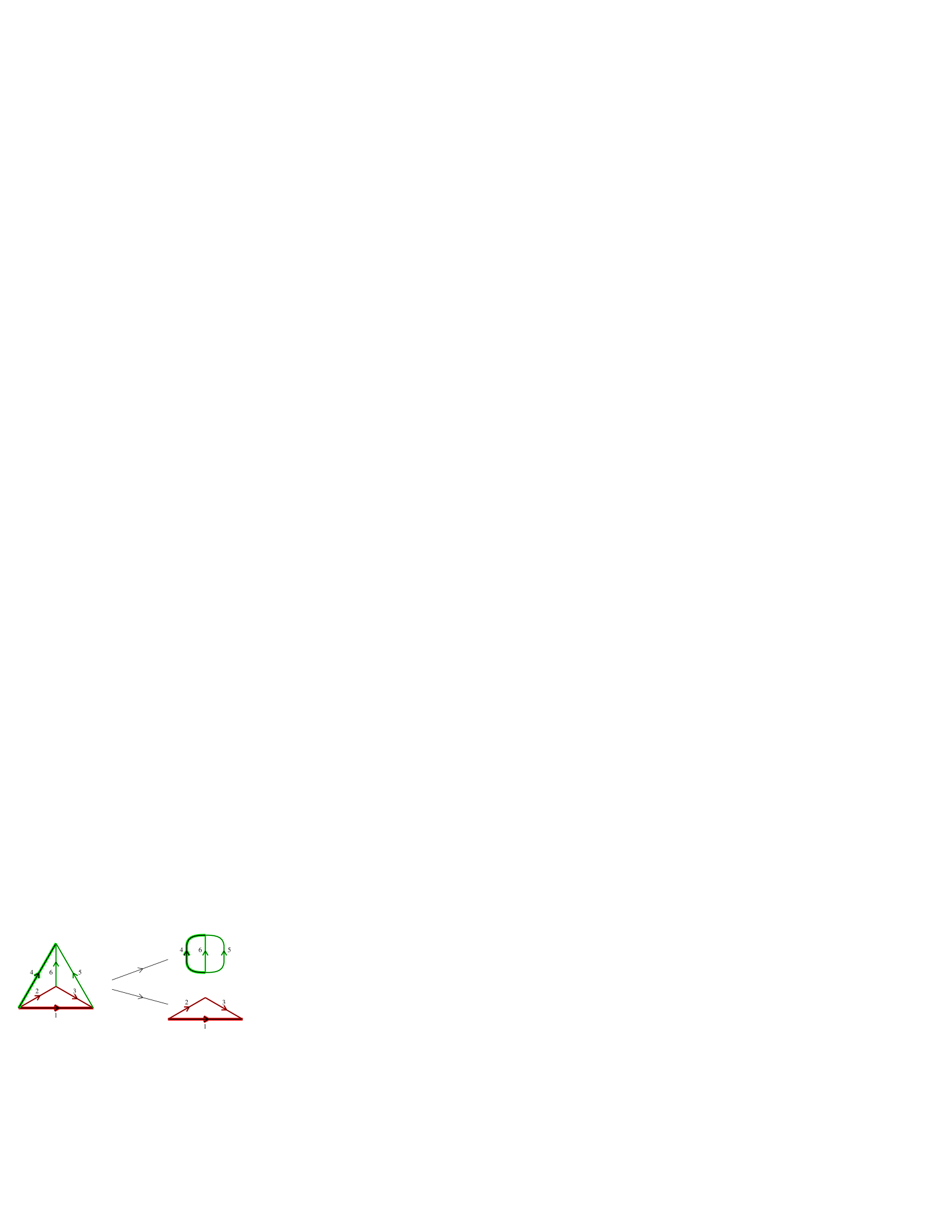
Figure 2: Active decomposition of an ordered acyclic digraph ${\overrightarrow{G}}$ (on the left). The active filtration is $\emptyset=F_{c}\subset 123\subset 123456$ (Definition 3.3). The active partition is $123+456$, with cyclic flat $F_{c}=\emptyset$ (Definition 3.4). The active minors (in the middle) are ${\overrightarrow{G}}(123456)/123$, which is bipolar w.r.t. $4$, and ${\overrightarrow{G}}(123)$, which is bipolar w.r.t. $1$ (Definition 3.6). On the right part, we show the four digraphs in the same activity class (Definition 3.19). They share the same active partition/filtration, and the same active minors up to reorienting all their edges.

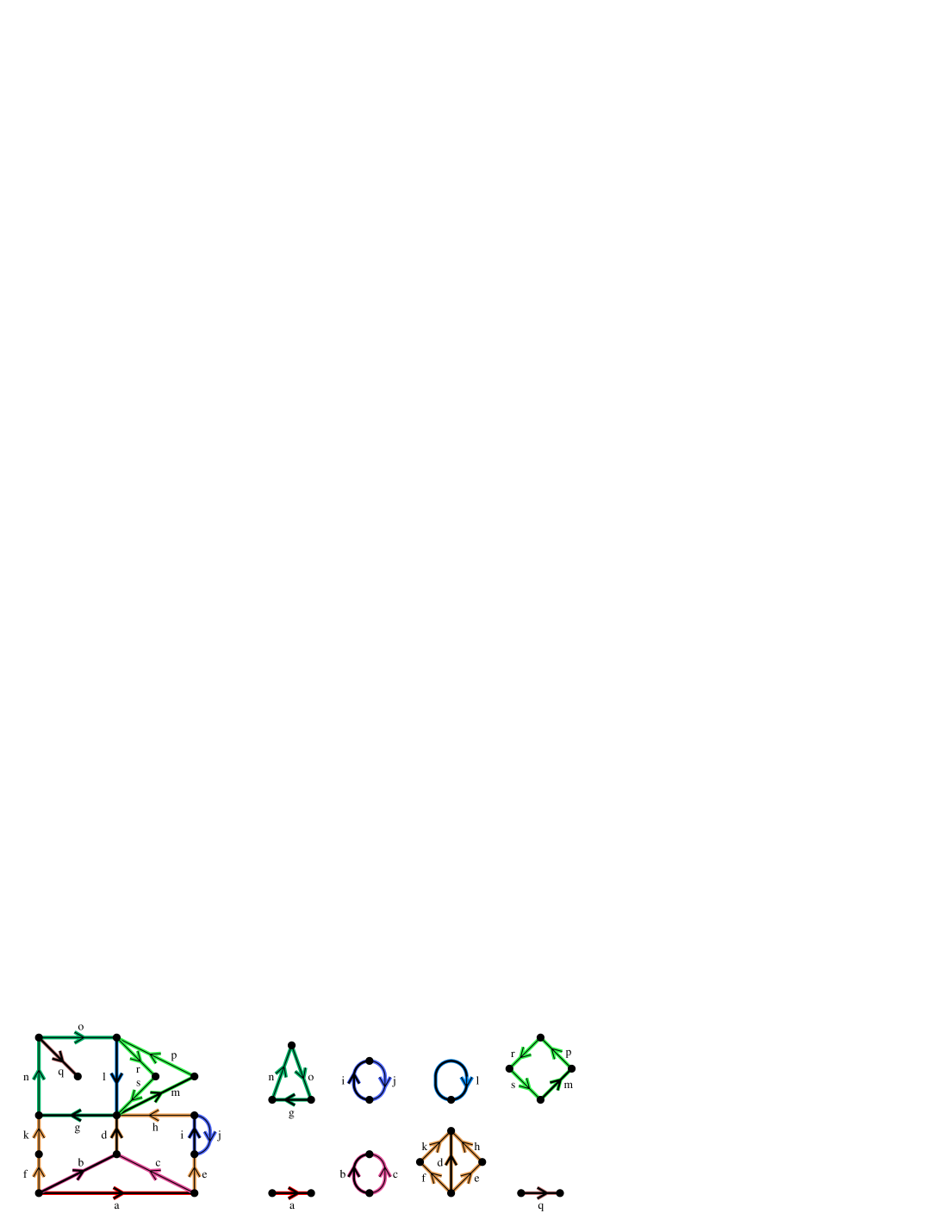
Figure 3: Active decomposition of an ordered digraph ${\overrightarrow{G}}$ (shown on the left). The ordering of $E$ is given by: $a<b<c<\dots<q<r<s$. The active partition is given by: $F_{c}=gno+ij+l+mprs$ and $E\setminus F_{c}=a+bc+defhk+q$ (Definition 3.4). In particular, the active edges are $O({\overrightarrow{G}})=\{g,i,l,m\}$ and the dual-active edges are $O^{*}({\overrightarrow{G}})=\{a,b,d,q\}$ (bold edges). The bipolar, resp. cyclic-bipolar, active minors w.r.t. their smallest edges, whose edge sets are given by the active partition, are shown in the bottom right line, resp. the upper right line (Definition 3.6).

Recall that $\subset$ denotes a strict inclusion. See Section 2.6 for properties of cycles and cocycles in minors, and for some terminology (e.g. cyclic flats), inherited from classical matroid theory.

Definition 3.3.

Let ${\overrightarrow{G}}$ be an ordered directed graph, with $\iota$ dual-active edges $a_{1}<...<a_{\iota}$ and $\varepsilon$ active edges $a^{\prime}_{1}<...<a^{\prime}_{\varepsilon}$. The active filtration of ${\overrightarrow{G}}$ is the sequence of subsets of $E$:

$$\emptyset=F^{\prime}_{\varepsilon}\subset F^{\prime}_{\varepsilon-1}\subset\ldots\subset F^{\prime}_{0}=F_{c}=F_{0}\subset\ldots\subset F_{\iota-1}\subset F_{\iota}=E,$$

that can be also denoted $(F^{\prime}_{\varepsilon},\ldots,F^{\prime}_{0},F_{c},F_{0},\ldots,F_{\iota})$, defined by the following. The subset $F_{c}$, called the cyclic flat of the sequence, is

$$F_{c}\ =\ \bigcup_{C\hbox{\small\ directed cycle}}C\ =\ E\ \setminus\ \bigcup_{C\hbox{\small\ directed cocycle}}C.$$

We have $F_{\iota}=E$, and for every $0\leq k\leq\iota-1$, we have

$$F_{k}=E\ \setminus\ \bigcup_{\begin{subarray}{c}D\hbox{\small\ directed cocycle}\\ {{\small\mathrm{min}}}(D)\;\geq\;a_{k+1}\end{subarray}}D.$$

We have $F^{\prime}_{\varepsilon}=\emptyset$, and for every $0\leq k\leq\varepsilon-1$, we have

$$F^{\prime}_{k}=\bigcup_{\begin{subarray}{c}C\hbox{\small\ directed cycle}\\ {{\small\mathrm{min}}}(C)\;\geq\;a^{\prime}_{k+1}\end{subarray}}C.$$

One can note that, for $0\leq k\leq\iota$, $F_{k}$ is a flat of $G$ and, for $0\leq k\leq\varepsilon$, $F^{\prime}_{k}$ is a dual flat of $G$ .

Definition 3.4.

The active partition of ${\overrightarrow{G}}$ is the partition of $E$ induced by successive differences of sets in the active filtration:

$$E=(F^{\prime}_{\varepsilon-1}\setminus F^{\prime}_{\varepsilon})\ \uplus\ \dots\ \uplus\ (F^{\prime}_{0}\setminus F^{\prime}_{1})\ \uplus\ (F_{1}\setminus F_{0})\ \uplus\ \dots\ \uplus\ (F_{\iota}\setminus F_{\iota-1}),$$

with:

$\begin{array}[]{ll}\mathrm{min}(F^{\prime}_{k-1}\setminus F^{\prime}_{k})=a^{\prime}_{k}&\text{for }1\leq k\leq\varepsilon,\\[2.84526pt] \mathrm{min}(F_{k}\setminus F_{k-1})=a_{k}&\text{for }1\leq k\leq\iota.\end{array}$

We assume that the active partition is always given with the cyclic flat $F_{c}$ (i.e. it can be thought of as a pair of partitions, one for $F_{c}$, the other for $E\setminus F_{c}$). For convenience, we can refer to $F_{c}$, or to the parts forming $F_{c}$, as the cyclic part of ${\overrightarrow{G}}$, and to $E\setminus F_{c}$, or to the parts forming $E\setminus F_{c}$, as the acyclic part of ${\overrightarrow{G}}$.

Observe that knowing the subsets forming the active partition of ${\overrightarrow{G}}$ allows us to build the active filtration of ${\overrightarrow{G}}$. Indeed, the sequence $\mathrm{min}(F_{k}\setminus F_{k-1})$, $1\leq k\leq\iota$, is increasing with $k$, and the sequence $\mathrm{min}(F^{\prime}_{k-1}\setminus F^{\prime}_{k})$, $1\leq k\leq\varepsilon$, is increasing with $k$, so the position of each part of the active partition with respect to the active filtration is identified. Also, we have, for $1\leq k\leq\iota$,

$$F_{k}\setminus F_{k-1}=\bigcup_{\begin{subarray}{c}D\hbox{\small\ directed cocycle}\\ {{\small\mathrm{min}}}(D)\;=\;a_{k}\end{subarray}}D\ \ \setminus\ \bigcup_{\begin{subarray}{c}D\hbox{\small\ directed cocycle}\\ {{\small\mathrm{min}}}(D)\;>\;a_{k}\end{subarray}}D,$$

and, for $1\leq k\leq\varepsilon$,

$$F^{\prime}_{k-1}\setminus F^{\prime}_{k}=\bigcup_{\begin{subarray}{c}D\hbox{\small\ directed cycle}\\ {{\small\mathrm{min}}}(D)\;=\;a^{\prime}_{k}\end{subarray}}D\ \ \setminus\ \bigcup_{\begin{subarray}{c}D\hbox{\small\ directed cycle}\\ {{\small\mathrm{min}}}(D)\;>\;a^{\prime}_{k}\end{subarray}}D.$$

Let us point out that the particular case of acyclic digraphs is addressed as the case where $F_{c}=\emptyset$, and the strongly connected case is addressed as the case where $F_{c}=E$. Those cases can be thought of as being dual to each other (they are actually dual in an oriented matroid setting). By the same token, in the planar case, $(F^{\prime}_{\varepsilon},\ldots,F^{\prime}_{0},F_{c},F_{0},\ldots,F_{\iota})$ is the active filtration of ${\overrightarrow{G}}$ if and only if $(E\setminus F_{\iota},\ldots,E\setminus F_{0},E\setminus F_{c},E\setminus F^{\prime}_{0},\ldots,E\setminus F^{\prime}_{\varepsilon})$ is the active filtration of a dual ${\overrightarrow{G}}^{*}$ of ${\overrightarrow{G}}$ (which is the reason for the symmmetry in the two subscript orderings). Also, one can see that if the active filtration of ${\overrightarrow{G}}$ is $(F^{\prime}_{\varepsilon},\ldots,F^{\prime}_{0},F_{c},F_{0},\ldots,F_{\iota})$ then the active filtration of ${\overrightarrow{G}}(F_{c})$ (strongly connected digraph) is $\emptyset=F^{\prime}_{\varepsilon}\subset F^{\prime}_{\varepsilon-1}\subset\ldots\subset F^{\prime}_{0}=F_{c}=F_{c},$ and the active filtration of ${\overrightarrow{G}}/F_{c}$ (acyclic digraph) is $\emptyset=F_{c}\setminus F_{c}=F_{0}\setminus F_{c}\subset\ldots\subset F_{\iota-1}\setminus F_{c}\subset F_{\iota}\setminus F_{c}=E\setminus F_{c}$ (an extensive refinement of these properties is provided in Observation 3.13 below).

Remark 3.5.

As shown in [20, Section 7], the notion of active partition for an ordered digraph generalizes the notion of components of acyclic orientations with a unique sink. This last notion, studied in [35] in relation with the chromatic polynomial, in [45] in terms of heaps of pieces, and in [7] in terms of non-commutative monoids (see also [13]), relies on certain linear orderings of the vertex set. For every such vertex ordering, there exists a consistent edge ordering such that active partitions exactly match acyclic orientation components. Our generalization allows us to consider any orientation and any ordering of the edge set (along with a generalization to oriented matroids).

Definition 3.6.

The active minors of ${\overrightarrow{G}}$ are the minors

$${\overrightarrow{G}}(F_{k})/F_{k-1},\text{ for }1\leq k\leq\iota,\text{ and }$$

$${\overrightarrow{G}}(F^{\prime}_{k-1})/F^{\prime}_{k},\text{ for }1\leq k\leq\varepsilon.\hphantom{\text{ and }}$$

Proposition 3.7.

With the notations of Definitions 3.3, and 3.6, we have:

• the $\iota$ active minors ${\overrightarrow{G}}(F_{k})/F_{k-1}$, $1\leq k\leq\iota,$ are bipolar w.r.t. $a_{k}=\mathrm{min}(F_{k}\setminus F_{k-1})$,

• the $\varepsilon$ active minors ${\overrightarrow{G}}(F^{\prime}_{k-1})/F^{\prime}_{k}$, $1\leq k\leq\varepsilon,$ are cyclic-bipolar w.r.t. $a^{\prime}_{k}=\mathrm{min}(F^{\prime}_{k-1}\setminus F^{\prime}_{k})$.

Proof.

Direct by recursively using Lemma 3.8 below. ∎

Lemma 3.8.

We use the notations of Definitions 3.3. If $\iota>0$ then, denoting $F=F_{\iota-1}$, we have:

• ${\overrightarrow{G}}/F$ is bipolar with respect to $a_{\iota}$,

• the active filtration of ${\overrightarrow{G}}(F)$ is $(F^{\prime}_{\varepsilon},\ldots,F^{\prime}_{0},F_{c},F_{0},\ldots,F_{\iota-1})$.

If $\varepsilon>0$ then, denoting $F^{\prime}=F^{\prime}_{\varepsilon-1}$, we have:

• ${\overrightarrow{G}}(F^{\prime})$ is cyclic-bipolar with respect to $a^{\prime}_{\varepsilon}$,

• the active filtration of ${\overrightarrow{G}}/F^{\prime}$ is $(F^{\prime}_{\varepsilon-1}\setminus F^{\prime},\ldots,F^{\prime}_{0}\setminus F^{\prime},F_{c}\setminus F^{\prime},F_{0}\setminus F^{\prime},\ldots,F_{\iota}\setminus F^{\prime})$.

Proof.

The proof separately deals with the two parts of the statement. We begin with the second part, in which we assume $\varepsilon>0$ and handle cycles. The other half of the proof, in which we assume $\iota>0$ and handle cocycles, is dual from the previous one. In an oriented matroid setting, we would not have to prove the two halves, we would just have to apply one half to the dual (see [26]). Here, in a graph setting, we have to adapt it. Essentially, the dual part consists in replacing terms and constructions with their dual corresponding ones, except that a supplementary technicality is used to handle cocycles. Also, recall that cycles and cocycles of $G$ and of its minors are all considered as subsets of $E$.

— Cycles part. Assume $\varepsilon>0$ and let $F^{\prime}=F^{\prime}_{\varepsilon-1}$. The cycles of ${\overrightarrow{G}}(F^{\prime})$ are the cycles of ${\overrightarrow{G}}$ contained in $F^{\prime}$, where $F^{\prime}$ is the union of all directed cycles $C$ of ${\overrightarrow{G}}$ with smallest edge $a^{\prime}_{\varepsilon}$. Hence every edge of ${\overrightarrow{G}}(F^{\prime})$ belongs to a directed cycle, hence ${\overrightarrow{G}}(F^{\prime})$ is totally cyclic. And $a^{\prime}_{\varepsilon}$ belongs to a directed cycle of ${\overrightarrow{G}}(F^{\prime})$, hence $a^{\prime}_{\varepsilon}$ is active in ${\overrightarrow{G}}(F^{\prime})$. If another element was active in ${\overrightarrow{G}}(F^{\prime})$, then it would also be the smallest element of a directed cycle in ${\overrightarrow{G}}$ and active in ${\overrightarrow{G}}$, a contradiction with $a^{\prime}_{\varepsilon}$ being the greatest active element of ${\overrightarrow{G}}$. So we have $O({\overrightarrow{G}}(F^{\prime}))=\{a^{\prime}_{\varepsilon}\}$ and $O^{*}({\overrightarrow{G}}(F^{\prime}))=\emptyset$, that is: ${\overrightarrow{G}}(F^{\prime})$ is cyclic-bipolar with respect to $a^{\prime}_{\varepsilon}$.

As $F^{\prime}$ is a union of directed cycles of ${\overrightarrow{G}}$, the directed cocycles of ${\overrightarrow{G}}/F^{\prime}$ are the directed cocycles of ${\overrightarrow{G}}$. Hence, ${\overrightarrow{G}}$ and ${\overrightarrow{G}}/F^{\prime}$ have the same dual-active edges and the same unions of directed cocycles with given smallest element. Hence, the “dual part” $(F_{c},F_{0},\ldots,F_{\iota-1},F_{\iota}=E)$ of their active filtration is the same up to removing $F^{\prime}$ from each subset.

The cycles of ${\overrightarrow{G}}/F^{\prime}$ are exactly the non-empty inclusion-minimal intersections of cycles of ${\overrightarrow{G}}$ with $E\setminus F^{\prime}$. More precisely, the signed subsets of the form $C\setminus F^{\prime}$, where $C$ is a cycle of ${\overrightarrow{G}}$, are unions of cycles of ${\overrightarrow{G}}/F^{\prime}$. Since every element of $F^{\prime}$ is greatest than $a^{\prime}_{\varepsilon}$ by definition of $a^{\prime}_{\varepsilon}$, we have that $a^{\prime}_{k}\in E\setminus F^{\prime}$ for every $1\leq k<\varepsilon$. A directed cycle $C$ of ${\overrightarrow{G}}$ with smallest element $a^{\prime}_{k}$, for $1\leq k<\varepsilon$, induces a directed cycle of $G/F^{\prime}$ contained in $C\setminus F^{\prime}$ with smallest element $a^{\prime}_{k}$, hence $a^{\prime}_{1},\dots,a^{\prime}_{\varepsilon-1}$ are active in ${\overrightarrow{G}}/F^{\prime}$. Let $H^{\prime}_{k}=\cup\{C\mid C\hbox{ directed cycle of }{\overrightarrow{G}}/F^{\prime},\ \mathrm{min}(D)>a^{\prime}_{k}\}$. Independently, by definition of $F^{\prime}_{k}$, we have $F^{\prime}_{k}\setminus F^{\prime}=\cup\{C\setminus F^{\prime}\mid C\hbox{ directed cycle of }{\overrightarrow{G}},\ \mathrm{min}(C)>a^{\prime}_{k}\}$. For every directed cycle $C$ of ${\overrightarrow{G}}$, $C\setminus F^{\prime}$ is a union of directed cycles of $G/F^{\prime}$, so we have $F^{\prime}_{k}\setminus F^{\prime}\subseteq H^{\prime}_{k}$.

Now, conversely, let $e$ be an element of $H^{\prime}_{k}$, for some $1\leq k<\varepsilon$. It belongs to be a directed cycle $C$ of ${\overrightarrow{G}}/F^{\prime}$ with smallest element $a>a^{\prime}_{k}$. As $F^{\prime}$ is a union of directed cycles of ${\overrightarrow{G}}$, it is easy to see that there exists a directed cycle $C^{\prime}$ of ${\overrightarrow{G}}$ containing $e$ and contained in $C\cup F^{\prime}$. Since every element of $F^{\prime}$ is greater than $a^{\prime}_{\varepsilon}$ and $a^{\prime}_{\varepsilon}\geq a>a^{\prime}_{k}$, the smallest element of $C^{\prime}$ is greater than $a$, hence strictly greater than $a^{\prime}_{k}$. Since $e$ belongs to $C^{\prime}\setminus F^{\prime}$, we get that $e\in F^{\prime}_{k}\setminus F^{\prime}$. We have proved $H^{\prime}_{k}\subseteq F^{\prime}_{k}\setminus F^{\prime}$, that is finally $F^{\prime}_{k}\setminus F^{\prime}\subseteq H^{\prime}_{k}$, which provides the active filtration of ${\overrightarrow{G}}/F^{\prime}$.

— Cocycles dual part. Assume $\iota>0$ and let $F=F_{\iota-1}$. The cocycles of ${\overrightarrow{G}}/F$ are the cocycles of ${\overrightarrow{G}}$ contained in $E\setminus F$, where $E\setminus F$ is the union of all directed cocycles $D$ of ${\overrightarrow{G}}$ with smallest edge $a_{\iota}$. Hence every edge of ${\overrightarrow{G}}/F$ belongs to a directed cocycle, hence ${\overrightarrow{G}}/F$ is acyclic. And $a_{\iota}$ belongs to a directed cocycle of ${\overrightarrow{G}}/F$, hence $a_{\iota}$ is dual-active in ${\overrightarrow{G}}/F$. If another element was dual-active in ${\overrightarrow{G}}/F$, then it would also be the smallest element of a directed cocycle in ${\overrightarrow{G}}$ and dual-active in ${\overrightarrow{G}}$, a contradiction with $a_{\iota}$ being the greatest dual-active element of ${\overrightarrow{G}}$. So we have $O^{*}({\overrightarrow{G}}/F)=\{a_{\iota}\}$ and $O({\overrightarrow{G}}/F)=\emptyset$, that is ${\overrightarrow{G}}/F$ is bipolar with respect to $a_{\iota}$.

As $E\setminus F$ is a union of directed cocycles of ${\overrightarrow{G}}$, the directed cycles of ${\overrightarrow{G}}(F)$ are the directed cycles of ${\overrightarrow{G}}$. Hence, ${\overrightarrow{G}}$ and ${\overrightarrow{G}}(F)$ have the same active edges, and the “primal part” $(F^{\prime}_{\varepsilon},\ldots,F^{\prime}_{0},F_{c})$ of their active filtration is the same.

The cocycles of ${\overrightarrow{G}}(F)$ are exactly the non-empty inclusion-minimal intersections of intersections of $F$ and cocycles of ${\overrightarrow{G}}$. More precisely, the signed subsets of the form $C\cap F$, where $C$ is a cocycle of ${\overrightarrow{G}}$, are unions of cocycles of ${\overrightarrow{G}}(F)$. Since every element of $E\setminus F$ is greatest than $a_{\iota}$ by definition of $a_{\iota}$, we have that $a_{k}\in F$ for every $1\leq k<\iota$. A directed cocycle $D$ of ${\overrightarrow{G}}$ with smallest element $a_{k}$, for $1\leq k<\iota$, induces a directed cocycle contained in $D\cap F$ of $G(F)$ with smallest element $a_{k}$, hence $a_{1},\dots,a_{\iota-1}$ are dual-active in ${\overrightarrow{G}}(F)$. Let $H_{k}=F\setminus\cup\{D\mid D\hbox{ directed cocycle of }{\overrightarrow{G}}(F),\ \mathrm{min}(D)>a_{k}\}$. Independently, by definition of $F_{k}$, we have $F_{k}=F\cap F_{k}=F\setminus\cup\{F\cap D\mid D\hbox{ directed cocycle of }{\overrightarrow{G}},\ \mathrm{min}(D)>a_{k}\}$. For every directed cocycle $D$ of ${\overrightarrow{G}}$, $D\cap F$ is a union of directed cocycles of $G(F)$, so we have $F\setminus F_{k}\subseteq F\setminus H_{k}$, that is $H_{k}\subseteq F_{k}$.

Now, conversely, let $e$ be an element of $F\setminus H_{k}$, for some $1\leq k<\iota$. It belongs to be a directed cocycle $D$ of ${\overrightarrow{G}}(F)$ with smallest element $a>a_{k}$. We want to prove that $e$ belongs to $F\cap D^{\prime}$ for some directed cocycle $D^{\prime}$ of ${\overrightarrow{G}}$ contained in $D\cup(E\setminus F)$. This is less easy to see than for cycles as in the above part of the proof. We give a proof using usual oriented matroid technique. Let us recall that the composition $A\circ B$ between two signed edge subsets as the edge subset $A\cup B$ with signs inherited from $A$ for the element of $A$ and inherited from $B$ for the elements of $B\setminus A$. The cocycle $D$ is contained in a cocycle $D_{G}$ of ${\overrightarrow{G}}$ with $D_{G}\cap F=D$. Let $D^{\prime}_{G}$ be the composition of all directed cocycles of ${\overrightarrow{G}}$ with smallest element $a_{\iota}$, whose support is $E\setminus F$ and whose signs are all positive (since given by directed cocycles). Then $D^{\prime}_{G}\circ D_{G}$ is positive, since it is positive on $E\setminus F$ as $D^{\prime}_{G}$, and positive on $D_{G}\cap F=D$ as $D$. And $D^{\prime}_{G}\circ D_{G}$ has smallest element $a$, since $a<a_{\iota}$. By the conformal composition property of covectors in oriented matroid theory, there exists a directed cocycle $D^{\prime}$ of ${\overrightarrow{G}}$ containing $e$ and contained in $D_{G}\cup(E\setminus F)$. Since every element of $E\setminus F$ is greater than $a_{\iota}$ and $a_{\iota}\geq a>a_{k}$, the smallest element of $D^{\prime}$ is greater than $a$, hence strictly greater than $a_{k}$. Since $e$ belongs to $F\cap D^{\prime}$, we get that $e\in F\setminus F_{k}$. We have proved $F\setminus H_{k}\subseteq F\setminus F_{k}$, that is finally $F_{k}=H_{k}$, which provides the active filtration of ${\overrightarrow{G}}(F)$. ∎

3.2 Decomposition of the set of all orientations of an ordered graph - Tutte polynomial in terms of filtrations and beta invariants of minors

Let us now characterize and build on the set of all possible sequences of subsets that can be active filtrations of an orientation of a given graph, and let us obtain general results involving all orientations of the underlying graph, not only a given directed graph. After giving definitions for these sequences, we first complete Proposition 3.7 with a uniqueness property in Proposition 3.12, then we extend this result to a bijective result taking into account all possible sequences in Theorem 3.14, whose enumerative counterpart is the Tutte polynomial formula of Theorem 3.15.

Definition 3.9.

Let $E$ be a linearly ordered set. Let $G=(V,E)$ be a graph with set of edges $E$. We call filtration of $G$ (or of $E$) a sequence $(F^{\prime}_{\varepsilon},\ldots,F^{\prime}_{0},F_{c},F_{0},\ldots,F_{\iota})$ of subsets of $E$ such that:

• $\emptyset=F^{\prime}_{\varepsilon}\subset...\subset F^{\prime}_{0}=F_{c}=F_{0}\subset...\subset F_{\iota}=E$;

• the sequence $\mathrm{min}(F_{k}\setminus F_{k-1})$, $1\leq k\leq\iota$ is increasing with $k$;

• the sequence $\mathrm{min}(F^{\prime}_{k-1}\setminus F^{\prime}_{k})$, $1\leq k\leq\varepsilon$, is increasing with $k$.

For convenience, in the rest of the paper, we can equally use the notations $(F^{\prime}_{\varepsilon},\ldots,F^{\prime}_{0},F_{c},F_{0},\ldots,F_{\iota})$ or $\emptyset=F^{\prime}_{\varepsilon}\subset...\subset F^{\prime}_{0}=F_{c}=F_{0}\subset...\subset F_{\iota}=E$ to denote a filtration of $G$.

Definition 3.10.

A filtration $(F^{\prime}_{\varepsilon},\ldots,F^{\prime}_{0},$ $F_{c},F_{0},\ldots,F_{\iota})$ of $G$ is called connected if, in addition:

• for every $1\leq k\leq\iota$, the minor $G(F_{k})/F_{k-1}$ is either loopless and 2-connected with at least two edges, or a single isthmus;

• for every $1\leq k\leq\varepsilon$, the minor $G(F^{\prime}_{k-1})/F^{\prime}_{k}$ is either loopless and 2-connected with at least two edges, or a single loop.

The minors involved in Definition 3.10 are said to be associated with or induced by the filtration. Let us recall that the 2-connectivity of a graph means its 2-vertex connectivity, and that we consider a loopless graph on two vertices with at least one edge as 2-connected (Section 2.1). Let us recall that, for a graph $G$ with at least two edges, $G$ is loopless 2-connected if and only if $\beta(G)\not=0$ if and only if $\beta^{*}(G)\not=0$ (if and only if there exists a bipolar orientation of $G$ if and only if there exists a cyclic-bipolar orientation of $G$ if and only if the cycle matroid of $G$ is connected, see Section 2.4). Let us lastly recall that, for a graph $G$ with one edge, we have $\beta(G)=1$ and $\beta^{*}(G)=0$ if it is an isthmus, and $\beta(G)=0$ and $\beta^{*}(G)=1$ if it is a loop. From these results, we derive the next lemma.

Lemma 3.11.

A filtration $(F^{\prime}_{\varepsilon},\ldots,F^{\prime}_{0},$ $F_{c},F_{0},\ldots,F_{\iota})$ of $G$ is connected if and only if

$\displaystyle\Bigl{(}\prod_{1\leq k\leq\iota}\beta\bigl{(}G(F_{k})/F_{k-1}\bigr{)}\Bigr{)}\ \Bigl{(}\prod_{1\leq k\leq\varepsilon}\beta^{*}\bigl{(}G(F^{\prime}_{k-1})/F^{\prime}_{k}\bigr{)}\Bigr{)}\ \not=\ 0.$ ∎

Proposition 3.12.

Let ${\overrightarrow{G}}$ be an ordered directed graph. The active filtration of ${\overrightarrow{G}}$ is the unique (connected) filtration $(F^{\prime}_{\varepsilon},\ldots,F^{\prime}_{0},F_{c},F_{0},\ldots,F_{\iota})$ of $G$ such that the $\iota$ minors

$${\overrightarrow{G}}(F_{k})/F_{k-1},\ \ 1\leq k\leq\iota,$$

are bipolar with respect to $a_{k}=\mathrm{min}(F_{k}\setminus F_{k-1})$, and the $\varepsilon$ minors

$${\overrightarrow{G}}(F^{\prime}_{k-1})/F^{\prime}_{k},\ \ 1\leq k\leq\varepsilon,$$

are cyclic-bipolar with respect to $a^{\prime}_{k}=\mathrm{min}(F^{\prime}_{k-1}\setminus F^{\prime}_{k})$.

Proof.

First, we check that the active filtration $\emptyset=F^{\prime}_{\varepsilon}\subset...\subset F^{\prime}_{0}=F_{c}=F_{0}\subset...\subset F_{\iota}=E$ of ${\overrightarrow{G}}$ is a filtration of $G$. Assume ${\overrightarrow{G}}$ has $\iota$ dual-active edges $a_{1}<...<a_{\iota}$, and $\varepsilon$ active edges $a^{\prime}_{1}<...<a^{\prime}_{\varepsilon}$. By definition of $a_{k}$, for $1\leq k\leq\iota$, there exists a directed cocycle of ${\overrightarrow{G}}$ whose smallest element is $a_{k}$, hence $a_{k}\in F_{k}\setminus F_{k-1}$ according to the definition of $F_{k}\setminus F_{k-1}$ given above. So we have $a_{k}=\mathrm{min}(F_{k}\setminus F_{k-1})$, $1\leq k\leq\iota$, which is increasing with $k$ by definition of $a_{k}$. Similarly, for $1\leq k\leq\varepsilon$, there exists a directed cycle of ${\overrightarrow{G}}$ whose smallest element is $a^{\prime}_{k}$, so we get $a^{\prime}_{k}=\mathrm{min}(F^{\prime}_{k-1}\setminus F^{\prime}_{k})$, which is increasing with $k$. Hence the result.

Second, by Proposition 3.7, the active minors exactly satisfy the property stated in the statement. This also proves that those minors are loopless and 2-connected as soon as they have more than one edge, which shows that the active filtration of ${\overrightarrow{G}}$ is a connected filtration of $G$.

Now, it remains to prove the uniqueness property. Assume $(F^{\prime}_{\varepsilon},\ldots,F^{\prime}_{0},F_{c},F_{0},\ldots,F_{\iota})$ is a filtration of $E$ satisfying the properties given in the statement. Then it is obviously a connected filtration of $G$, by the definitions, since being bipolar, resp. cyclic-bipolar, implies being either connected or reduced to an isthmus, resp. a loop. First, we prove that $F_{c}$ is the union of all directed cycles of ${\overrightarrow{G}}$. Assume $C$ is a directed cycle of ${\overrightarrow{G}}$, not contained in $F_{c}$. Let $k$ be the smallest such that $C\subseteq F_{k}$, $1\leq k\leq\iota$. Then $C\setminus F_{k-1}\not=\emptyset$ (otherwise $k$ would not be minimal), so $C\setminus F_{k-1}$ contains a directed cycle of ${\overrightarrow{G}}/F_{k-1}$. Moreover $C\setminus F_{k-1}\subseteq F_{k}\setminus F_{k-1}$ by definition of $k$, so $C\setminus F_{k-1}$ contains a directed cycle of ${\overrightarrow{G}}_{k}={\overrightarrow{G}}(F_{k})/F_{k-1}$, a contradiction with ${\overrightarrow{G}}_{k}$ being acyclic. Hence the union of directed cycles of ${\overrightarrow{G}}$ is contained in $F_{c}$. With exactly the same reasoning from the dual viewpoint, we get that the union of directed cocycles of ${\overrightarrow{G}}$ is contained in $E\setminus F_{c}$. Precisely: assume $D$ is a directed cocycle of ${\overrightarrow{G}}$, not contained in $E\setminus F_{c}$. Let $k$ be the smallest such that $D\subseteq E\setminus F^{\prime}_{k}$, $1\leq k\leq\varepsilon$. Then $D\cap F^{\prime}_{k-1}\not=\emptyset$ (otherwise $k$ would not be minimal), so $D\cap F^{\prime}_{k-1}$ contains a directed cocycle of ${\overrightarrow{G}}(F^{\prime}_{k-1})$. Moreover $D\cap F^{\prime}_{k-1}\subseteq F^{\prime}_{k-1}\setminus F^{\prime}_{k}$ by definition of $k$, so $D\cap F^{\prime}_{k-1}$ contains a directed cocycle of ${\overrightarrow{G}}^{\prime}_{k}={\overrightarrow{G}}(F^{\prime}_{k-1})/F^{\prime}_{k}$, a contradiction with ${\overrightarrow{G}}^{\prime}_{k}$ being strongly connected. Finally, $F_{c}$ contains the union of directed cycles of ${\overrightarrow{G}}$ and has an empty intersection with the union of all directed cocycles of ${\overrightarrow{G}}$, so $F_{c}$ is exactly the union of all directed cycles of ${\overrightarrow{G}}$.

Second, we prove the following claim: for every directed cycle $C$ of ${\overrightarrow{G}}$, the smallest element of $C$ equals $a^{\prime}_{k+1}$, where $k$ is the greatest possible such that $C\subseteq F^{\prime}_{k}$, $0\leq k\leq\varepsilon-1$. Indeed, for such $C$ and $k$, we have $C\setminus F^{\prime}_{k+1}\not=\emptyset$ (otherwise $k$ would not be maximal), so $C\setminus F^{\prime}_{k+1}$ is a union of directed cycles of ${\overrightarrow{G}}/F^{\prime}_{k+1}$. Moreover, $C\setminus F^{\prime}_{k+1}\subseteq F^{\prime}_{k}\setminus F^{\prime}_{k+1}$ by definition of $k$, so $C\setminus F^{\prime}_{k+1}$ is a union of directed cycles of ${\overrightarrow{G}}^{\prime}_{k+1}={\overrightarrow{G}}(F^{\prime}_{k})/F^{\prime}_{k+1}$. By assumption that ${\overrightarrow{G}}^{\prime}_{k+1}$ is cyclic-bipolar with respect to $a^{\prime}_{k+1}$, we have that $a^{\prime}_{k+1}$ belongs to every directed cycle of ${\overrightarrow{G}}^{\prime}_{k+1}$, so $a^{\prime}_{k+1}$ is the smallest edge of $C\setminus F^{\prime}_{k+1}$. By definition of a filtration, $a^{\prime}_{k+1}$ is the smallest edge in $F^{\prime}_{k}$ (it is the smallest in $F^{\prime}_{k}\setminus F^{\prime}_{k+1}$ and the sequence $\mathrm{min}(F^{\prime}_{i}\setminus F^{\prime}_{i+1})$ is increasing with $i$), hence we have $\mathrm{min}(C)=a^{\prime}_{k+1}$. In particular, we have proved that the active edges of ${\overrightarrow{G}}$ are of type $a^{\prime}_{k}$, $1\leq k\leq\varepsilon$.

Dually, we prove - the same way - the following claim: for every directed cocycle $D$ of ${\overrightarrow{G}}$, the smallest element of $D$ equals $a_{k+1}$, where $k$ is the greatest possible such that $D\subseteq E\setminus F_{k}$, $0\leq k\leq\iota-1$. Indeed, for such $D$ and $k$, we have $D\cap F_{k+1}\not=\emptyset$ (otherwise $k$ would not be maximal), so $D\cap F_{k+1}$ is a union of directed cocycles of ${\overrightarrow{G}}(F_{k+1})$. Moreover, $D\cap F_{k+1}\subseteq F_{k+1}\setminus F_{k}$ by definition of $k$, so $D\cap F_{k+1}$ is a union of directed cocycles of ${\overrightarrow{G}}_{k+1}={\overrightarrow{G}}(F_{k+1})/F_{k}$. By assumption that ${\overrightarrow{G}}_{k+1}$ is bipolar with respect to $a_{k+1}$, we have that $a_{k+1}$ belongs to every directed cocycle of ${\overrightarrow{G}}_{k+1}$, so $a_{k+1}$ is the smallest edge of $D\cap F_{k+1}$. By definition of a filtration, $a_{k+1}$ is the smallest edge in $E\setminus F_{k}$ (it is the smallest in $F_{k}\setminus F_{k-1}$ and the sequence $\mathrm{min}(F_{i}\setminus F_{i-1})$ is increasing with $i$), hence we have $\mathrm{min}(C)=a_{k+1}$. In particular, we have proved that the dual-active edges of ${\overrightarrow{G}}$ are of type $a_{k}$, $1\leq k\leq\iota$.

Third, we prove that the parts of the considered filtration are indeed the parts of the active filtration. Let us denote $F=F_{\varepsilon-1}$ and so $a^{\prime}_{\varepsilon}=\mathrm{min}(F)$. We want to prove that $F=\cup\{C\mid C\hbox{ directed cycle of }{\overrightarrow{G}},\ \mathrm{min}(C)=a^{\prime}_{\varepsilon}\}$. By assumption, $G^{\prime}_{\varepsilon}={\overrightarrow{G}}(F)$ is cyclic-bipolar. So, every edge of ${\overrightarrow{G}}(F)$ belongs to a directed cycle of ${\overrightarrow{G}}(F)$ with smallest element $a^{\prime}_{\varepsilon}$. The cycles of ${\overrightarrow{G}}(F)$ are the cycles of ${\overrightarrow{G}}$ contained in $F$. Hence, every edge of ${\overrightarrow{G}}$ belonging to $F$ belongs to a directed cycle of ${\overrightarrow{G}}$ with smallest element $a^{\prime}_{\varepsilon}$, which proves that $F\subseteq\cup\{C\mid C\hbox{ directed cycle of }{\overrightarrow{G}},\ \mathrm{min}(C)=a^{\prime}_{\varepsilon}\}$. Conversely, let $C$ be a directed cycle of ${\overrightarrow{G}}$ with smallest element $a^{\prime}_{\varepsilon}$. By the above claim, we have that $\varepsilon-1$ is the greatest possible such that $D\subseteq F^{\prime}_{\varepsilon-1}$, that is $D\subseteq F$, hence the result.

Dually, let us denote $F=F_{\iota-1}$ and so $a_{\iota}=\mathrm{min}(E\setminus F)$. We want to prove that $F=E\setminus\cup\{D\mid D\hbox{ directed cocycle of }{\overrightarrow{G}},\ \mathrm{min}(D)=a_{\iota}\}$. By assumption, $G_{\iota}={\overrightarrow{G}}/F$ is bipolar. So, every edge of ${\overrightarrow{G}}/F$ belongs to a directed cocycle of ${\overrightarrow{G}}/F$ with smallest element $a_{\iota}$. The cocycles of ${\overrightarrow{G}}/F$ are the cocycles of ${\overrightarrow{G}}$ contained in $E\setminus F$. Hence, every edge of ${\overrightarrow{G}}$ belonging to $E\setminus F$ belongs to a directed cocycle of ${\overrightarrow{G}}$ with smallest element $a_{\iota}$, which proves that $E\setminus F\subseteq\cup\{D\mid D\hbox{ directed cocycle of }{\overrightarrow{G}},\ \mathrm{min}(D)=a_{\iota}\}$. Conversely, let $D$ be a directed cocycle of ${\overrightarrow{G}}$ with smallest element $a_{\iota}$. By the above claim, we have that $\iota-1$ is the greatest possible such that $D\subseteq E\setminus F_{\iota-1}$, that is $D\subseteq E\setminus F$, hence the result.

Now, we can conclude by induction, assuming the proposition is true for minors of ${\overrightarrow{G}}$. Assume $\iota>0$ and denote again $F=F_{\iota-1}$, we have proved above that $F$ is indeed the largest part different from $E$ in the active filtration of ${\overrightarrow{G}}$. It is easy to check that the sequence of subsets $(F^{\prime}_{\varepsilon},\ldots,F^{\prime}_{0},F_{c},F_{0},\ldots,F_{\iota}-1)$ is a filtration of $G(F)$. Moreover this filtration obviously satisfies the properties of the proposition for the directed graph ${\overrightarrow{G}}(F)$, as the involved minors are unchanged. Hence, this filtration is the active filtration of ${\overrightarrow{G}}(F)$, by induction assumption. Hence, by Lemma 3.8, we have that the subsets $F^{\prime}_{\varepsilon},\ldots,F^{\prime}_{0},F_{c},F_{0},\ldots,F_{\iota}-1$ are indeed the same subsets as in the active filtration of ${\overrightarrow{G}}$. Finally, assume that $\varepsilon>0$ and denote again $F^{\prime}=F_{\varepsilon-1}$, we have proved above that $F^{\prime}$ is indeed the largest part different from $\emptyset$ in the active filtration of ${\overrightarrow{G}}$. It is easy to check that the sequence of subsets $(F^{\prime}_{\varepsilon-1}\setminus F^{\prime},\ldots,F^{\prime}_{0}\setminus F^{\prime},F_{c}\setminus F^{\prime},F_{0}\setminus F^{\prime},\ldots,F_{\iota}\setminus F^{\prime})$ is a filtration of $G/F^{\prime}$. Moreover this filtration obviously satisfies the properties of the proposition for the directed graph ${\overrightarrow{G}}/F^{\prime}$, as the involved minors are unchanged. Hence, this filtration is the active filtration of ${\overrightarrow{G}}/F^{\prime}$, by induction assumption. Hence, by Lemma 3.8, we have that the subsets $F^{\prime}_{\varepsilon-1},\ldots,F^{\prime}_{0},F_{c},F_{0},\ldots,F_{\iota}$ are indeed the same subsets as in the active filtration of ${\overrightarrow{G}}$. ∎

Observation 3.13.

Let $\emptyset=F^{\prime}_{\varepsilon}\subset...\subset F^{\prime}_{0}=F_{c}=F_{0}\subset...\subset F_{\iota}=E$ be the active filtration of ${\overrightarrow{G}}$. Let $F^{\prime}$ and $F$ be two subsets in this sequence such that $F^{\prime}\subseteq F$ (with possibly $F\subseteq F_{c}$ or $F_{c}\subseteq F^{\prime}$). Then, by Proposition 3.12, the active filtration of ${\overrightarrow{G}}(F)/F^{\prime}$ is obtained from the subsequence with extremities $F^{\prime}$ and $F$ (i.e. $F^{\prime}\subset\dots\subset F$) of the active filtration of ${\overrightarrow{G}}$ by subtracting $F^{\prime}$ from each subset of the subsequence (with $F_{c}\setminus F^{\prime}$ as cyclic flat). In particular, the subsequence ending with $F$ (i.e. $\emptyset\subset\dots\subset F$) yields the active filtration of $M(F)$, and the subsequence beginning with $F$ (i.e. $F\subset\dots\subset E$) yields the active filtration of $M/F$ by subtracting $F$ from each subset.

Theorem 3.14.

Let $G$ be an ordered graph. We have

$\Bigl{\{}\ \hbox{orientations ${\overrightarrow{G}}$ of $G$}\ \Bigr{\}}\$

$$=\ \biguplus\ \Biggl{\{}\ {\overrightarrow{G}}\ \ \mid\ \ G(F_{k})/F_{k-1},\ \ 1\leq k\leq\iota,\hbox{ bipolar with respect to }\mathrm{min}(F_{k}\setminus F_{k-1}),$$

$$\hphantom{\Biggl{\{}\ {\overrightarrow{G}}\ \ \mid\ \ }\hbox{and}\ \ {\overrightarrow{G}}(F^{\prime}_{k-1})/F^{\prime}_{k},\ \ 1\leq k\leq\varepsilon,\hbox{ cyclic-bipolar with respect to }\mathrm{min}(F^{\prime}_{k-1}\setminus F^{\prime}_{k})\ \ \Biggr{\}}.$$

where the disjoint union is over all connected filtrations $(F^{\prime}_{\varepsilon},\ldots,F^{\prime}_{0},F_{c},F_{0},\ldots,F_{\iota})$ of $G$. The connected filtration of $G$ associated to an orientation ${\overrightarrow{G}}$ in the right-hand side of the equality is the active filtration of ${\overrightarrow{G}}$.

Proof.

This result consists in a bijection between all orientations ${\overrightarrow{G}}$ of $G$ and sequences of orientations of the minors involved in decomposition sequences of $G$. It is directly given by Proposition 3.12. From the first set to the second set, the active filtration of ${\overrightarrow{G}}$ provides the required decomposition. Conversely, from the second set to the first set, first choose a connected filtration of $G$. Then, for each minor of $G$ defined by this sequence, choose a bipolar/cyclic-bipolar orientation for this minor as written in the second set statement. This defines an orientation ${\overrightarrow{G}}$ of $G$ (since every edge of $G$ appears in one and only one of these minors). Now, for this orientation ${\overrightarrow{G}}$, the chosen filtration satisifies the property of Proposition 3.12, hence this filtration is the active filtration of this orientation ${\overrightarrow{G}}$ of $G$. Finally, the uniqueness in Proposition 3.12 ensures that the union in the second set is disjoint. ∎

Theorem 3.15.

Let $G$ be a graph on a linearly ordered set of edges $E$. We have

$$t(G;x,y)=\ \ \sum\ \ \Bigl{(}\prod_{1\leq k\leq\iota}\beta\bigl{(}G(F_{k})/F_{k-1}\bigr{)}\Bigr{)}\ \Bigl{(}\prod_{1\leq k\leq\varepsilon}\beta^{*}\bigl{(}G(F^{\prime}_{k-1})/F^{\prime}_{k}\bigr{)}\Bigr{)}\ {x^{\iota}\ y^{\varepsilon}}$$

where $\beta^{*}=\beta$ for a graph with at least two edges, $\beta^{*}$ of a loop equals $1$, $\beta^{*}$ of an isthmus equals $0$, and where the sum can be equally:

• either over all connected filtrations $(F^{\prime}_{\varepsilon},\ldots,F^{\prime}_{0},F_{c},F_{0},\ldots,F_{\iota})$ of $G$;

• or over all filtrations $(F^{\prime}_{\varepsilon},\ldots,F^{\prime}_{0},F_{c},F_{0},\ldots,F_{\iota})$ of $E$.

Proof.

By Lemma 3.11, we directly have that the sum over all filtrations and the sum over all connected filtrations yield the same result. The result where the sum is over all connected filtrations of $G$ is exactly the enumerative translation of Theorem 3.14. More precisely, consider the set of orientations ${\overrightarrow{G}}$ with dual-activity $\iota$ and activity $\varepsilon$, whose cardinality is $o_{\iota,\varepsilon}$. This set bijectively corresponds to the set $\biguplus\bigl{\{}{\overrightarrow{G}}\mid{\overrightarrow{G}}(F_{k})/F_{k-1},\ \ 1\leq k\leq\iota,$ $\hbox{bipolar with respect to }\mathrm{min}(F_{k}\setminus F_{k-1}),$ $\hbox{ and }\ {\overrightarrow{G}}(F^{\prime}_{k-1})/F^{\prime}_{k},\ \ 1\leq k\leq\varepsilon,$ cyclic-bipolar with respect $\hbox{to }\mathrm{min}(F^{\prime}_{k-1}\setminus F^{\prime}_{k})\ \bigr{\}}$ where the union is over all connected filtrations of $G$ with fixed $\iota$ and $\varepsilon$. The cardinality of each part of this set is obviously $\Bigl{(}\prod_{1\leq k\leq\iota}2.\beta\bigl{(}G(F_{k})/F_{k-1}\bigr{)}\Bigr{)}\ \Bigl{(}\prod_{1\leq k\leq\varepsilon}2.\beta^{*}\bigl{(}G(F^{\prime}_{k-1})/F^{\prime}_{k}\bigr{)}\Bigr{)}$ since $\beta$ counts half the number of bipolar or cyclic-bipolar orientations of a graph with more than two edges, $\beta=1$ for a graph with a single isthmus (which can happen for minors of type $G(F_{k})/F_{k-1}$), and $\beta^{*}=1$ for a graph with a single loop (which can happen for minors of type $G(F^{\prime}_{k-1})/F^{\prime}_{k}$). To achieve the proof, we use that the coefficient $t_{\iota,\varepsilon}$ of the Tutte polynomial equals $o_{\iota,\varepsilon}/{2^{\iota+\varepsilon}}$, as shown in [38] (see Section 2.3). ∎

Remark 3.16.

From Proposition 3.7, we already have that any orientation ${\overrightarrow{G}}$ can be decomposed into bipolar/cyclic-bipolar minors induced by a (connected) filtration of $G$ (the active one of ${\overrightarrow{G}}$). Then we could directly deduce a weaker version of Theorem 3.14 with a union instead of a disjoint union, and a weaker version of Theorem 3.15 with an inequality instead of an equality. It is the uniqueness result of Proposition 3.12 that allows us to state Theorems 3.14 and 3.15 as they are.

Corollary 3.17 ([11, 33]).

Let $G$ be a graph. We have

$$t(G;x,y)=\sum t(G/F_{c};x,0)\ t(G(F_{c});0,y)$$

where the sum can be either over all subsets $F_{c}$ of $E$, or over all cyclic flats $F_{c}$ of $G$.

Proof.

By fixing $y=0$ in Theorem 3.15, we get

$t(G;x,0)=\ \ \sum\ \ \Bigl{(}\prod_{1\leq k\leq\iota}\beta\bigl{(}G(F_{k})/F_{k-1}\bigr{)}\Bigr{)}\ {x^{\iota}}$

where the sum is over all connected filtrations of type $\emptyset=F^{\prime}_{0}=F_{c}=F_{0}\subset\ldots\subset F_{\iota}=E$ of $G$. By fixing $x=0$, we get

$t(G;0,y)=\ \ \sum\ \ \ \Bigl{(}\prod_{1\leq k\leq\varepsilon}\beta^{*}\bigl{(}G(F^{\prime}_{k-1})/F^{\prime}_{k}\bigr{)}\Bigr{)}\ {y^{\varepsilon}}$

where the sum is over all connected filtrations of type $\emptyset=F^{\prime}_{\varepsilon}\subset\ldots\subset F^{\prime}_{0}=F_{c}=F_{0}=E$ of $G$. For a given cyclic flat $F_{c}$ of $G$, pairs of connected filtrations of $G/F_{c}$ and $G(F_{c})$ of the above type, respectively for $y=0$ and $x=0$, obviously correspond to the connected filtrations of $G$ of type $(F^{\prime}_{\varepsilon},\ldots,F^{\prime}_{0},$ $F_{c},F_{0},\ldots,F_{\iota})$ involving this $F_{c}$ (note that the subset $F_{c}$ in a connected filtration has to be a cyclic flat of the graph, since it is the cyclic flat of some active partition, see also the similar observation below Definition 3.4 in terms of the active filtration). Then, by decomposing the sum in Theorem 3.15 as $\sum_{F_{c}}\sum_{i,j}\Pi_{1\leq k\leq\iota}\dots\Pi_{1\leq k\leq\varepsilon}\dots$, we get the formula $t(G;x,y)=\sum t(G/F_{c};x,0)\ t(G(F_{c});0,y)$ where the sum is over all cyclic flats $F_{c}$ of $G$. If $F_{c}$ is not a cyclic flat, then either $G/F_{c}$ has a loop or $G(F_{c})$ has an isthmus, implying that the corresponding term in the sum equals zero. ∎

The formula in Corollary 3.17 is called convolution formula for the Tutte polynomial in [33], and it is also the enumerative translation of the bijection given in [11]. For information, we mention that Corollary 3.17 can also be proved very shortly and directly for graphs, using the enumeration of orientation activities formula of the Tutte polynomial from [38] (see Section 2.3), along with the fact that a digraph ${\overrightarrow{G}}$ can be uniquely decomposed into an acyclic digraph ${\overrightarrow{G}}/F_{c}$ and a strongly connected digraph ${\overrightarrow{G}}(F_{c})$ where $F_{c}$ is the union of directed cycles of ${\overrightarrow{G}}$ (however, such a proof does not generalize to non-orientable matroids). The reader can complete details or find them in [17]. Let us also mention that an algebraic proof of the formula in Theorem 3.15 could be obtained using matroid set functions, a technique introduced in [34], according to its author [36].

3.3 Activity classes in the set of all orientations of an ordered graph - Tutte polynomial expansion in terms of four refined orientation activities

Let us continue to build on active partitions. We define the notion of activity classes of orientations of an ordered graph. They are a central concept in this paper, and they will be put in bijection with spanning trees by the canonical active bijection in Section 4.2 (as in [20]). Next, we develop this notion to derive further structural and enumerative results, which are interesting on their own and will be used later for the refined active bijection in Section 4.3. Let us mention that the whole content of this section is generalized to oriented matroid perspectives in [15].

Proposition 3.18.

Let ${\overrightarrow{G}}$ be a directed graph on a linearly ordered set of edges $E$, with $\iota$ dual-active edges and $\varepsilon$ active edges. The $2^{\iota+\varepsilon}$ orientations of $G$ obtained by reorienting any union of parts of the active partition of ${\overrightarrow{G}}$ have the same active filtration/partition as ${\overrightarrow{G}}$ (and hence also the same active and dual-active edges, and the same active minors up to taking the opposite).

Proof.

The result is not difficult to prove directly from Definition 3.3: consider $A$ the union of all directed cycles (or cocycles) of ${\overrightarrow{G}}$ whose smallest edge is greater than a given edge $e$, and prove that every union of all directed cycles (or cocycles) whose smallest edge is greater than any edge is the same in ${\overrightarrow{G}}$ and $-_{A}{\overrightarrow{G}}$. We leave this proof as an exercise (see [26] for a similar short proof in oriented matroid terms, see [15] for a detailed more general proof in oriented matroid perspectives). Alternatively, the result can also be seen as a direct corollary of Theorem 3.14 or Proposition 3.12. Indeed, reorienting a union of parts of the active partition of ${\overrightarrow{G}}$ implies reorienting completely some of the active minors of ${\overrightarrow{G}}$. Then, for the resulting orientation, the resulting minors still satisfie the property of Proposition 3.12, hence the active filtration is the same as that of ${\overrightarrow{G}}$. ∎

Definition 3.19.

We call (orientation) activity class of ${\overrightarrow{G}}$ the set of all orientations of $G$ obtained by reorienting any union of parts of the active partition of ${\overrightarrow{G}}$.

An illustration is given in Figure 2. From Proposition 3.18, we directly get the following result.

Proposition 3.20.

Activity classes of orientations of $G$ partition the set of orientations of $G$:

$\displaystyle\bigl{\{}\ \text{orientations of }G\ \bigr{\}}=\biguplus_{\begin{subarray}{c}\text{activity classes}\\ \text{of orientations of }G\\ \text{\tiny(one $-_{A}{\overrightarrow{G}}$ chosen in each class)}\end{subarray}}\Bigl{\{}\ 2^{|O(-_{A}{\overrightarrow{G}})|+|O^{*}(-_{A}{\overrightarrow{G}})|}\ \ \begin{subarray}{c}\text{\small orientations obtained by}\\ \text{\small active partition reorienting}\end{subarray}\ \Bigr{\}}.$

∎

Definition 3.21.

Let ${\overrightarrow{G}}$ be a digraph on a linearly set of edges $E$ (thought of as a reference orientation of the graph $G$). Let $A\subseteq E$. The digraph $-_{A}{\overrightarrow{G}}$ is said to be active-fixed, resp. dual-active fixed, (with respect to ${\overrightarrow{G}}$) if the directions of all active, resp. dual-active, edges of $-_{A}{\overrightarrow{G}}$ agree with their directions in ${\overrightarrow{G}}$, that is if $O(-_{A}{\overrightarrow{G}})\cap A=\emptyset$, resp. $O^{*}(-_{A}{\overrightarrow{G}})\cap A=\emptyset.$

From Propositions 3.18 and 3.20, the Tutte polynomial formula in terms of orientations activities (Section 2.3), and the usual cyclic/acyclic decomposition, we derive the following counting results.

Corollary 3.22.

Let $G$ be an ordered graph. The number of activity classes of orientations of $G$ with activity $i$ and dual activity $j$ equals $t_{i,j}$.

Let ${\overrightarrow{G}}$ be a reference orientation of $G$. Each activity class of $G$ contains exactly one orientation of $G$ which is active-fixed and dual-active-fixed (w.r.t. ${\overrightarrow{G}}$). The number of such orientations of $G$ with activity $i$ and dual activity $j$ thus equals $t_{i,j}$.

In this way, we also obtain the enumerations given by Table 2. ∎

orientations of $G$ / activity classes of $G$	number
active-fixed and dual-active-fixed / all	$t(G;1,1)$
acyclic and dual-active-fixed / acyclic	$t(G;1,0)$
active-fixed and strongly connected / strongly connected	$t(G;0,1)$
active-fixed (/ non-applicable)	$t(G;2,1)$
dual-active-fixed (/ non-applicable)	$t(G;1,2)$

Table 2: Enumeration of certain orientations based on representatives of activity classes (Corollary 3.22).

Now, let us refine orientation activities into four parameters w.r.t. a reference orientation ${\overrightarrow{G}}$.

Definition 3.23.

Let ${\overrightarrow{G}}$ be an ordered directed graph (reference orientation of $G$). We define:

$$\Theta_{\overrightarrow{G}}(A) = O(-_{A}{\overrightarrow{G}})\setminus A,$$

$$\mkern 1.5mu\overline{\mkern-1.5mu\Theta\mkern-1.5mu}\mkern 1.5mu_{\overrightarrow{G}}(A) = O(-_{A}{\overrightarrow{G}})\cap A,$$

$$\Theta^{*}_{\overrightarrow{G}}(A) = O^{*}(-_{A}{\overrightarrow{G}})\setminus A,$$

$$\mkern 1.5mu\overline{\mkern-1.5mu\Theta\mkern-1.5mu}\mkern 1.5mu^{*}_{\overrightarrow{G}}(A) = O^{*}(-_{A}{\overrightarrow{G}})\cap A.$$

Hence we have $O(-_{A}{\overrightarrow{G}})=\Theta_{\overrightarrow{G}}(A)\uplus\mkern 1.5mu\overline{\mkern-1.5mu\Theta\mkern-1.5mu}\mkern 1.5mu_{\overrightarrow{G}}(A)$ and $O^{*}(-_{A}{\overrightarrow{G}})=\Theta^{*}_{\overrightarrow{G}}(A)\uplus\mkern 1.5mu\overline{\mkern-1.5mu\Theta\mkern-1.5mu}\mkern 1.5mu^{*}_{\overrightarrow{G}}(A)$.

These parameters can be seen as situating a reorientation of ${\overrightarrow{G}}$ in its activity class. Indeed, the representative $-_{A}{\overrightarrow{G}}$ of its activity class which is active-fixed and dual-active fixed (Corollary 3.22) satisfies $\mkern 1.5mu\overline{\mkern-1.5mu\Theta\mkern-1.5mu}\mkern 1.5mu_{\overrightarrow{G}}(A)=O(-_{A}{\overrightarrow{G}})\cap A=\emptyset$ and $\mkern 1.5mu\overline{\mkern-1.5mu\Theta\mkern-1.5mu}\mkern 1.5mu^{*}_{\overrightarrow{G}}(A)=O^{*}(-_{A}{\overrightarrow{G}})\cap A=\emptyset,$ and the other orientations in the same activity class correspond to other possible values of $\mkern 1.5mu\overline{\mkern-1.5mu\Theta\mkern-1.5mu}\mkern 1.5mu_{\overrightarrow{G}}(A)\subseteq O(-_{A}{\overrightarrow{G}})$ and $\mkern 1.5mu\overline{\mkern-1.5mu\Theta\mkern-1.5mu}\mkern 1.5mu^{*}_{\overrightarrow{G}}(A)\subseteq O^{*}(-_{A}{\overrightarrow{G}})$. A way of understanding the role of the reference orientation ${\overrightarrow{G}}$ is that it breaks the symmetry in each activity class, so that its boolean lattice structure can be expressed relatively to its aforemetioned representative. This feature will be taken up in Section 4.3 on the refined active bijection, in connection with the similar four parameters for spanning trees from Section 2.5. Let us also mention that, for suitable orderings (roughly when all branches of the smallest spanning tree are increasing), unique sink acyclic orientations are also representatives of their activity classes, see [20, Section 6].

Finally, we derive the following Tutte polynomial expansion formula in terms of these four parameters. A (technical) proof for Theorem 3.24 below is proposed in the preprint [40] by deletion/contraction in the more general setting of oriented matroid perspectives. As announced in [40], this theorem can be proved by means of the above construction on activity classes (this theorem can also be seen as a direct corollary of the similar formula for subset activities from Theorem 2.2 and the refined active bijection from Theorem 4.41). We give this short proof below for completeness of the paper, though it is a translation of the proof given in [15] for oriented matroid perspectives.

Theorem 3.24 ([40, 15]).

Let $G$ be a graph on a linearly ordered set of edges $E$, and ${\overrightarrow{G}}$ be an orientation of $G$. We have

$$T(G;x+u,y+v)=\sum_{A\subseteq E}\ x^{|\Theta^{*}_{\overrightarrow{G}}(A)|}\ u^{|\mkern 1.5mu\overline{\mkern-1.5mu\Theta\mkern-1.5mu}\mkern 1.5mu^{*}_{\overrightarrow{G}}(A)|}\ y^{|\Theta_{\overrightarrow{G}}(A)|}\ v^{|\mkern 1.5mu\overline{\mkern-1.5mu\Theta\mkern-1.5mu}\mkern 1.5mu_{\overrightarrow{G}}(A)|}.$$

Proof.

The proof is obtained by a simple combinatorial transformation. Let us start with the right-hand side of the equality, where we denote $\theta^{*}_{\overrightarrow{G}}(A)$ instead of $|\Theta^{*}_{\overrightarrow{G}}(A)|$, etc., by setting:

$$[Exp]=\sum_{A\subseteq E}x^{\theta^{*}_{\overrightarrow{G}}(A)}u^{\mkern 1.5mu\overline{\mkern-1.5mu\theta\mkern-1.5mu}\mkern 1.5mu^{*}_{\overrightarrow{G}}(A)}y^{\theta_{\overrightarrow{G}}(A)}v^{\mkern 1.5mu\overline{\mkern-1.5mu\theta\mkern-1.5mu}\mkern 1.5mu_{\overrightarrow{G}}(A)}.$$

Since $2^{E}$ is isomorphic to the set of orientations, which is partitioned into orientation activity classes of ${\overrightarrow{G}}$ (Proposition 3.20), and by choosing a representative for each activity class which is active-fixed an dual-active-fixed (as discussed above), we get:

$$[Exp]=\sum_{\begin{subarray}{c}\text{orientation activity classes of }G\\ \text{with one $-_{A}{\overrightarrow{G}}$ chosen in each class}\\ \text{such that $O(-_{A}{\overrightarrow{G}})\cap A=\emptyset$ and $O^{*}(-_{A}{\overrightarrow{G}})\cap A=\emptyset$}\end{subarray}}\ \ \sum_{\begin{subarray}{c}-_{A^{\prime}}{\overrightarrow{G}}\text{ in the }\\ \text{class of }-_{A}{\overrightarrow{G}}\end{subarray}}x^{\theta^{*}_{\overrightarrow{G}}(A^{\prime})}u^{\mkern 1.5mu\overline{\mkern-1.5mu\theta\mkern-1.5mu}\mkern 1.5mu^{*}_{\overrightarrow{G}}(A^{\prime})}y^{\theta_{\overrightarrow{G}}(A^{\prime})}v^{\mkern 1.5mu\overline{\mkern-1.5mu\theta\mkern-1.5mu}\mkern 1.5mu_{\overrightarrow{G}}(A^{\prime})}$$

As discussed above, when $-_{A^{\prime}}{\overrightarrow{G}}$ ranges the activity class of $-_{A}{\overrightarrow{G}}$, $\mkern 1.5mu\overline{\mkern-1.5mu\Theta\mkern-1.5mu}\mkern 1.5mu_{\overrightarrow{G}}(A^{\prime})$ and $\mkern 1.5mu\overline{\mkern-1.5mu\Theta\mkern-1.5mu}\mkern 1.5mu^{*}_{\overrightarrow{G}}(A^{\prime})$ range subsets of $O(-_{A}{\overrightarrow{G}})$ and $O^{*}(-_{A}{\overrightarrow{G}})$, respectively. So, we get the following expression (where “idem” refers to the text below the first above sum), which we then transform using the binomial formula:

$$[Exp] = \sum_{\text{idem}}\ \ \sum_{\begin{subarray}{c}P\subseteq O^{*}(-_{A}{\overrightarrow{G}})\\ Q\subseteq O(-_{A}{\overrightarrow{G}})\end{subarray}}x^{\mid O^{*}(-_{A}{\overrightarrow{G}})\setminus P\mid}u^{\mid P\mid}y^{\mid O(-_{A}{\overrightarrow{G}})\setminus Q\mid}v^{\mid Q\mid}$$

$$= \sum_{\text{idem}}\ \ \Biggl{(}\sum_{P\subseteq O^{*}(-_{A}{\overrightarrow{G}})}x^{\mid O^{*}(-_{A}{\overrightarrow{G}})\setminus P\mid}u^{\mid P\mid}\Biggr{)}\Biggl{(}\sum_{Q\subseteq O(-_{A}{\overrightarrow{G}})}y^{\mid O(-_{A}{\overrightarrow{G}})\setminus Q\mid}v^{\mid Q\mid}\Biggr{)}$$

$$= \sum_{\text{idem}}\ \ (x+u)^{|O^{*}(-_{A}{\overrightarrow{G}})|}(y+v)^{|O(-_{A}{\overrightarrow{G}})|}$$

Since the activity class of $-_{A}{\overrightarrow{G}}$ has ${2^{|O(-_{A}{\overrightarrow{G}})|+|O^{*}(-_{A}{\overrightarrow{G}})|}}$ elements with the same orientation activities, we have (denoting for short $o(A)=|O(-_{A}{\overrightarrow{G}})|$ and $o^{*}(A)=|O(-_{A}{\overrightarrow{G}})|$):

$$[Exp] = \sum_{\text{idem}}\ \ {1\over{2^{o(A)+o^{*}(A)}}}\ \sum_{\begin{subarray}{c}-_{A^{\prime}}{\overrightarrow{G}}\text{ in the class of }-_{A}{\overrightarrow{G}}\end{subarray}}\ (x+u)^{o^{*}(A^{\prime})}(y+v)^{o(A^{\prime})}$$

$$= \sum_{\text{idem}}\ \ \sum_{\begin{subarray}{c}-_{A^{\prime}}{\overrightarrow{G}}\text{ in the class of }-_{A}{\overrightarrow{G}}\end{subarray}}\ {\Bigl{(}{x+u\over 2}\Bigr{)}}^{o^{*}(A^{\prime})}{\Bigl{(}{y+v\over 2}\Bigr{)}}^{o(A^{\prime})}$$

$$= \sum_{A\subseteq E}\ {\Bigl{(}{x+u\over 2}\Bigr{)}}^{o^{*}(A)}{\Bigl{(}{y+v\over 2}\Bigr{)}}^{o(A)}$$

$$= t(G;x+u,y+v)$$

using at the end the orientation activity enumeration formula from [38] recalled in Section 2.3. ∎

Remark 3.25.

Numerous Tutte polynomial formulas can be obtained from Theorem 3.24, for instance by replacing variables ($x$, $u$, $y$, $v$) with $(x/2,x/2,y/2,y/2)$, or $(x+1,-1,y+1,-1)$, or $(2,0,0,0)$. One can also obtain expressions for Tutte polynomial derivatives. Such formulas, and a detailed example for this set of formulas, are given in [40] (see also [15, 17, 26]).

4 The three levels of the active bijection of an ordered graph

In this section, we give the definitions and main properties of the three levels of the active bijection, as depicted in the diagram of Figure 1 and as globally described in Section 1. We focus on the construction from digraphs/orientations to spanning trees/subsets. The inverse direction is summarized in Section 5.

4.1 The uniactive bijection - The fully optimal spanning tree of an ordered bipolar digraph

Let us recall or reformulate the precise definitions and main properties of the uniactive case of the active bijection, subject of [20, 24]. See Section 1 for a global introduction with related results.

Definition 4.26.

Let ${\overrightarrow{G}}=(V,E)$ be a directed graph, on a linearly ordered set of edges, which is bipolar with respect to the minimal element $p$ of $E$. The fully optimal spanning tree $\alpha({\overrightarrow{G}})$ of ${\overrightarrow{G}}$ is the unique spanning tree $T$ of $G$ such that:

$\bullet$ for all $b\in T\setminus\{p\}$, the directions (or the signs) of $b$ and $\mathrm{min}(C^{*}(T;b))$ are opposite in $C^{*}(T;b)$;

$\bullet$ for all $e\in E\setminus T$, the directions (or the signs) of $e$ and $\mathrm{min}(C(T;e))$ are opposite in $C(T;e)$.

Note that a directed graph and its opposite have the same fully optimal spanning tree. Let us mention that the above definition has equivalent formulations involving unions of successive fundamental cycles/cocycles [20, 24] (recalled in [29, Section LABEL:ABG2LP-subsec:prelim-fob]). A detailed illustration of the above definition on a bipolar orientation of $K_{4}$ is given in [26] (see also [20] for another example).

The existence and uniqueness of the fully optimal spanning tree is the main result of [20, 24]. This is a deep and tricky result with several intepretations, mainly geometrical (see [26, Section 5] for a recap). It is equivalent to the key theorem below, before which we give dual definitions extending the above one, and after which we give further precisions from the constructive viewpoint.

Definition 4.27 (Dual and very similar to Definition 4.26).

Let ${\overrightarrow{G}}=(V,E)$ be a directed graph on a linearly ordered set of edges, cyclic-bipolar with respect to the minimal element $p$ of $E$. We define $\alpha({\overrightarrow{G}})$ as the unique spanning tree $T$ of $G$ such that:

$\bullet$ for all $b\in T$, the directions (or signs) of $b$ and $\mathrm{min}(C^{*}(T;b))$ are opposite in $C^{*}(T;b)$;

$\bullet$ for all $e\in(E\setminus T)\setminus\{p\}$, the directions (or signs) of $e$ and $\mathrm{min}(C(T;e))$ are opposite in $C(T;e)$.

Definition 4.28 (equivalent to Definition 4.27).

Let ${\overrightarrow{G}}=(V,E)$ be a directed graph on a linearly ordered set of edges, cyclic-bipolar with respect to the minimal element $p$ of $E$. We assume $|E|>1$. Then $-_{p}{\overrightarrow{G}}$ has the property to be bipolar with respect to $p$, and we define $\alpha({\overrightarrow{G}})$ as:

$$\alpha({\overrightarrow{G}})=\alpha(-_{p}{\overrightarrow{G}})\setminus\{p\}\cup\{p^{\prime}\}$$ (Active Duality)

where $p^{\prime}$ is the smallest edge of $E$ distinct from $p$.

The equivalence of these two definitions is given by [24, Theorem 5.3]. Only the second one was used in [20]. Let us observe that Definition 4.27 comes from Definition 4.26 and cycle/cocycle duality. Actually, for a planar ordered graph ${\overrightarrow{G}}$, assumed to be (cyclic-)bipolar w.r.t. the smallest edge, and a dual ${\overrightarrow{G}}^{*}$ of ${\overrightarrow{G}}$, we have:

$$\alpha({\overrightarrow{G}})=E\setminus\alpha({{\overrightarrow{G}}}^{*}).$$ (Duality)

Then, the Active Duality property provided by Definition 4.28 means that Definitions 4.26 and 4.27 are compatible with the canonical bijection between bipolar and cyclic-bipolar orientations (see Section 2.3), and the canonical bijection between internal and external uniactive spanning trees (see Section 2.2), as detailed in [20, Section 4]. Let us mention that the Active Duality property can also be seen as a strengthening of linear programming duality, see [24, Section 5]. We sum up these duality properties of $\alpha$ in the diagram of Figure 4.

Figure 4: Commutative diagram of duality properties of the uniactive bijection in the planar case. It involves the usual duality ($\vec{G}^{*}$ is any planar dual of $\vec{G}$) and the active duality (Definition 4.28). It generalizes to general graphs using the oriented matroid dual $M^{*}(\vec{G})$ instead of $\vec{G}^{*}$ (and, beyond, to general oriented matroids [24, 26]).

Theorem 4.29 (Key Theorem [20, 24]).

Let $G$ be a graph on a linearly ordered set of edges $E$ with smallest edge $p$.

The mapping ${\overrightarrow{G}}\mapsto\alpha({\overrightarrow{G}})$ yields a bijection between all bipolar orientations of $G$ w.r.t. $p$ with fixed orientation for $p$ and all spanning trees of $G$ with internal activity $1$ and external activity $0$.

Also, it yields a bijection between all cyclic-bipolar orientations of $G$ w.r.t. $p$ with fixed orientation for $p$ and all spanning trees of $G$ with internal activity $0$ and external activity $1$.

The bijection provided by Theorem 4.29 is called the uniactive bijection of the ordered graph $G$. This bijection was built in [20, 24] by its inverse, from uniactive internal spanning trees to bipolar orientations, provided by a single pass algorithm over the spanning tree, or equally (dually) over its complement. Actually, it is easy to see that, given a uniactive spanning tree, one just has to choose orientations one by one in a single pass over $E$ (following the ordering) so as to build an orientation for which this spanning tree satisfies the criterion of Definition 4.26 or 4.27. We recall this algorithm in Proposition 5.47 in Section 5.2. The problem of computing the direct image of a bipolar ordered digraph under $\alpha$ is not easy, and it is precisely addressed in the companion paper [29]. An efficient but technical solution [29, Section LABEL:ABG2LP-sec:fob] uses a linear number of minors, and consists in an adaptation for graphs of a more general construction by means of elaborations on linear programming [23, 27]. Alternatively, the uniactive bijection $\alpha$ can also be built by deletion/contraction, quite naturally but using an exponential number of minors, see Section 6.1 and [29, Section LABEL:ABG2LP-sec:induction] for details. Let us emphasize that those two constructions of $\alpha$ do not give a proof of Theorem 4.29, or of the existence and uniqueness of $\alpha({\overrightarrow{G}})$ in Definition 4.26: on the contrary, this fundamental result is used to prove their correctness.

4.2 The canonical active bijection - The active spanning tree of an ordered digraph

First, we give three equivalent definitions for the active spanning tree of an ordered digraph, consistently with the definition given in [20]. Then, we give the main theorem stating the consistency and properties of the construction, yielding the canonical active bijection of an ordered graph. Then, we give its complete proof, that mainly makes the link between spanning trees and constructions of Section 3 for orientations. See Section 1 for a global introduction.

An important feature of the canonical active bijection is that it preserves active partitions, meaning that the active partition of a digraph is the same as the active partition of its active spanning tree. We will mention this second notion of active partition though it has not yet been defined in the paper. For convenience, we postpone this definition to Section 5.1 (it can be defined by several ways, the proof of the main theorem of this section will prove at the same time this spanning tree decomposition, which is also shortly defined in [20] and detailed in [25]).

An interesting underlying feature, that we will not develop in this paper, is how the active spanning tree is characterized by a sign criterion directly on its fundamental cycles/cocycles (obtained by applying the criterion for the uniactive case used in the previous section to suitable subsets of these cycles/cocycles obtained by the decomposition used in the present section, which also yields the algorithm of Section 5.2). We invite the reader to look at the several detailed examples in [26] of active spanning trees of orientations of the graph $K_{4}$ (which are consistent with the $K_{4}$ example in Section 7).

Definition 4.30.

Let ${\overrightarrow{G}}$ be a directed graph on a linearly ordered set of edges. The active spanning tree $\alpha({\overrightarrow{G}})$ is defined by extending the definition of $\alpha$ from (cyclic-)bipolar (Definitions 4.26 to 4.28) to general ordered digraphs by the two following characteristic properties:

(1) $\bullet$ $\alpha({\overrightarrow{G}})=\alpha({\overrightarrow{G}}/F)\ \uplus\ \alpha({\overrightarrow{G}}(F))$ where $F$ is the union of all directed cycles of ${\overrightarrow{G}}$ whose smallest element is the greatest active element of ${\overrightarrow{G}}$.

(2) $\bullet$ $\alpha({\overrightarrow{G}})=\alpha({\overrightarrow{G}}/F)\ \uplus\ \alpha({\overrightarrow{G}}(F))$ where $F$ is the complementary of the union of all directed cocycles of ${\overrightarrow{G}}$ whose smallest element is the greatest dual-active element of ${\overrightarrow{G}}$.

Let us briefly justify why $\alpha({\overrightarrow{G}})$ is well defined, by Lemma 3.8: in property (1), if $F\not=\emptyset$, then ${\overrightarrow{G}}(F)$ is cyclic-bipolar, and ${\overrightarrow{G}}/F$ has one active element less than ${\overrightarrow{G}}$; in property (2), if $E\setminus F\not=\emptyset$, then ${\overrightarrow{G}}/F$ is bipolar, and ${\overrightarrow{G}}(F)$ has one dual-active element less than ${\overrightarrow{G}}$. Then, the two properties are consistent and can be used recursively in any way, finally yielding the next definition.

Definition 4.31 (equivalent to Definition 4.30).

Let ${\overrightarrow{G}}$ be a directed graph on a linearly ordered set of edges, with active filtration $\emptyset=F^{\prime}_{\varepsilon}\subset...\subset F^{\prime}_{0}=F_{c}=F_{0}\subset...\subset F_{\iota}=E$. We define

$$\alpha({\overrightarrow{G}})=\ \biguplus_{1\leq k\leq\iota}\alpha\bigl{(}{\overrightarrow{G}}(F_{k})/F_{k-1}\bigr{)}\ \uplus\ \biguplus_{1\leq k\leq\varepsilon}\alpha\bigl{(}{\overrightarrow{G}}(F^{\prime}_{k-1})/F^{\prime}_{k}\bigr{)}.$$

Observe that this definition is valid since each active minor is either bipolar or cyclic-bipolar, by Proposition 3.7, and its image has been defined in Definitions 4.26 to 4.28. Observe also that the $2^{\iota+\varepsilon}$ digraphs in the same activity class as ${\overrightarrow{G}}$ have the same image under $\alpha$ as ${\overrightarrow{G}}$ (as they have the same active minors up to taking the opposite, cf. Proposition 3.18).

Observation 4.32.

Let us consider an ordered digraph ${\overrightarrow{G}}$ and continue Observation 3.13. Let $\emptyset=F^{\prime}_{\varepsilon}\subset...\subset F^{\prime}_{0}=F_{c}=F_{0}\subset...\subset F_{\iota}=E$ be the active filtration of ${\overrightarrow{G}}$. Let $F$ and $F^{\prime}$ be two subsets in this sequence such that $F^{\prime}\subseteq F$. In particular, $F^{\prime}$ can be a $F^{\prime}_{i}$, $0\leq i\leq\varepsilon$, that is any union of directed cycles whose smallest edge is greater than a given edge, and $F$ can be a $F_{i}$, $0\leq i\leq\iota$, that is the complementary of any union of directed cocycles whose smallest edge is greater than a given edge. Then, by Definition 4.31, we have

$$\alpha({\overrightarrow{G}})=\alpha\bigl{(}{\overrightarrow{G}}(F^{\prime})\bigr{)}\uplus\alpha\bigl{(}{\overrightarrow{G}}(F)/F^{\prime}\bigr{)}\uplus\alpha\bigl{(}{\overrightarrow{G}}/F\bigr{)}.$$

In this way, we can also derive the following equivalent relaxed definition.

Definition 4.33 (equivalent to Definitions 4.30 and 4.31).

Let ${\overrightarrow{G}}$ be an ordered directed graph. We define $\alpha({\overrightarrow{G}})$ by Definitions 4.26 to 4.28 if ${\overrightarrow{G}}$ is (cyclic-)bipolar w.r.t. its smallest edge, and by the following characteristic property:

$$\alpha({\overrightarrow{G}})=\alpha({\overrightarrow{G}}/F)\ \uplus\ \alpha({\overrightarrow{G}}(F))$$

where $F$ is either any union of all directed cycles of ${\overrightarrow{G}}$ whose smallest edge is greater than a fixed edge of ${\overrightarrow{G}}$, or the complementary of any union of all directed cocycles of ${\overrightarrow{G}}$ whose smallest edge is greater than a fixed edge of ${\overrightarrow{G}}$.

Let us finally observe that the definition of $\alpha$ is consistent with cycle/cocycle duality. For a dual pair of planar graphs ${\overrightarrow{G}}$ and ${\overrightarrow{G}}^{*}$, this is expressed the following way:

$$\alpha({\overrightarrow{G}})=E\setminus\alpha({{\overrightarrow{G}}}^{*})$$ (Duality)

(which is also valid for general graphs by replacing ${\overrightarrow{G}}^{*}$ with the dual oriented matroid $M^{*}({\overrightarrow{G}})$).

Theorem 4.34.

Let $G$ be a graph on a linearly ordered set of edges $E$.

1. For any orientation ${\overrightarrow{G}}$ of $G$, $\alpha({\overrightarrow{G}})$ is well defined, and Definitions 4.30, 4.31 and 4.33 are equivalent.

2. For any orientation ${\overrightarrow{G}}$ of $G$, $\alpha({\overrightarrow{G}})$ is a spanning tree of $G$ with the same active filtration as ${\overrightarrow{G}}$ (Definitions 3.3 in Section 3.1, and 5.44 in Section 5.1), which implies in particular

   $$\mathrm{Int}\bigl{(}\alpha({\overrightarrow{G}})\bigr{)} = O^{*}({\overrightarrow{G}}),$$

   $$\mathrm{Ext}\bigl{(}\alpha({\overrightarrow{G}})\bigr{)} = O({\overrightarrow{G}}).$$

3. The $2^{i+j}$ orientations of $G$ in a given activity class with activity $j$ and dual-activity $i$ are mapped onto the same spanning tree by $\alpha$.

4. The mapping ${\overrightarrow{G}}\mapsto\alpha({\overrightarrow{G}})$ from orientations of $G$ to spanning trees of $G$ is surjective. It provides a bijection between all activity classes of orientations of $G$ and all spanning trees of $G$ (see Table 1 in Section 1 for noticeable restrictions).

The bijection provided by Theorem 4.34 is called the canonical active bijection of the ordered graph $G$. Observe that it depends only on $G$ and its edge-set ordering, not on a particular orientation ${\overrightarrow{G}}$ of $G$. Let us mention that the inverse mapping can be computed by a single pass over $E$, see Section 5.2 (and let us mention a deletion/contraction construction, see Section 6.2).

The rest of the section is devoted to proving Theorem 4.34. Using the decomposition for orientations from Theorem 3.14 and the bijection in the bipolar case from Theorem 4.29, we can prove Theorem 4.34 by means of two lemmas establishing the link with spanning trees, and we can derive at the same time a decomposition for spanning trees. This decomposition will be stated later as Theorem 5.43 and will yield equivalent definitions of the active filtration of a spanning tree in Definition 5.44, see Section 5. Let us observe that this last decomposition generalizes to matroid bases [25], but such proofs based on orientations are not possible in non-orientable matroids.

Property 4.35.

Let $T$ be a spanning tree of a graph $G$ with set of edges $E$. Let $B\subset A\subseteq E$. Assume $T^{\prime}=T\cap A\setminus B$ is a spanning tree of $G^{\prime}=G(A)/B$. Then, for all $b\in T^{\prime}$, we have

$$C^{*}_{G^{\prime}}(T^{\prime};b)=C^{*}_{G}(T;b)\cap A=C^{*}_{G}(T;b)\cap A\setminus B,$$

and, for all $e\in(A\setminus B)\setminus T^{\prime}$, we have

$$C_{G^{\prime}}(T^{\prime};e)=C_{G}(T;e)\setminus B=C_{G}(T;e)\cap A\setminus B.$$

Proof.

Direct by the definitions and the properties of cycles and cocycles in minors. ∎

Lemma 4.36.

Let ${\overrightarrow{G}}$ be an ordered digraph. Then, $\alpha({\overrightarrow{G}})$ is well defined by Definitions 4.30, 4.31 and 4.33, equivalently. Moreover, denoting $T=\alpha({\overrightarrow{G}})$, we have that $T$ is a spanning tree of $G$, with $\mathrm{Int}(T)=O^{*}({\overrightarrow{G}})$ and $\mathrm{Ext}(T)=O({\overrightarrow{G}})$.

Proof.

The fact that $\alpha({\overrightarrow{G}})$ is a well defined subset of $E$ and that Definitions 4.30, 4.31 and 4.33 of $\alpha({\overrightarrow{G}})$ are equivalent directly comes from the above discussion and from Section 3.1.

Using notations of Definition 4.31, Proposition 3.7 that ensures that the active minors are (cyclic-)bipolar, and Theorem 4.29 stating the active bijection for (cyclic-)bipolar orientations, we have $T=\alpha({\overrightarrow{G}})=\ \biguplus_{1\leq k\leq\iota}T_{k}\ \uplus\ \biguplus_{1\leq k\leq\varepsilon}T^{\prime}_{k}$, where, for $1\leq k\leq\iota$, $T_{i}=\alpha\bigl{(}{\overrightarrow{G}}(F_{k})/F_{k-1}\bigr{)}$ is a uniactive internal spanning tree of $G_{k}=G(F_{k})/F_{k-1}$, and, for $1\leq k\leq\varepsilon$, $T^{\prime}_{i}=\alpha\bigl{(}{\overrightarrow{G}}(F^{\prime}_{k-1})/F^{\prime}_{k}\bigr{)}$ is a uniactive external spanning tree of $G^{\prime}_{k}=G(F^{\prime}_{k-1})/F^{\prime}_{k}$. Recall that, for every subset $F\subseteq E$, the union of a spanning tree of $G/F$ and of a spanning tree of $G(F)$ is a spanning tree of $G$. Then a direct induction shows that $T$ is a spanning tree of $G$.

The directed graph ${\overrightarrow{G}}$ has $\iota\geq 0$ dual-active elements, which we denote $a_{1}<...<a_{\iota}$, and $\varepsilon\geq 0$ active elements, which we denote $a^{\prime}_{1}<...<a^{\prime}_{\varepsilon}$. Also, let us denote ${\mathcal{S}}=(F^{\prime}_{\varepsilon},\ldots,F^{\prime}_{0},F_{c},F_{0},\ldots,F_{\iota})$ the active filtration of ${\overrightarrow{G}}$.

— External activity part. Let us prove that $\mathrm{Ext}(T)=\{a^{\prime}_{1},\dots,a^{\prime}_{\varepsilon}\}$.

Let $e\in\mathrm{Ext}(T)$. By definition, $e\not\in T$ and $e=\mathrm{min}(C(T;e))$. Since ${\mathcal{S}}$ induces a partition of $E$, $e$ is an edge of a minor $H$ of $G$ induced by this sequence ${\mathcal{S}}$: either $H=G_{k}$ for some $1\leq k\leq\iota$ or $H=G^{\prime}_{k}$ for some $1\leq k\leq\varepsilon$. In any case, $e$ is an element of the spanning tree $T_{H}$ induced by $T$ in $H$: either $T_{H}=T_{k}$ if $H=G_{k}$, or $T_{H}=T^{\prime}_{k}$ if $H=G^{\prime}_{k}$. By Property 4.35, $C_{H}(T_{H};e)$ is obtained from $C_{G}(T;e)$ by removing elements not in the edge set of $H$. So $e=\mathrm{min}(C_{H}(T_{H};e))$, so $e$ is externally active in the spanning tree $T_{H}$ of the graph $H$. By properties of the spanning trees induced by $T$ in the minors induced by the sequence ${\mathcal{S}}$, this implies that $e=a^{\prime}_{k}$ for some $1\leq k\leq\varepsilon$. Hence $\mathrm{Ext}(T)\subseteq\{a^{\prime}_{1},\dots,a^{\prime}_{\varepsilon}\}$.

Conversely, let $1\leq k\leq\varepsilon$. By properties of the sequence ${\mathcal{S}}$, we have $a^{\prime}_{k}=\mathrm{min}(C_{G^{\prime}_{k}}(T_{k};a^{\prime}_{k}))$. As above, it is easy to see that we have $C_{G^{\prime}_{k}}(T_{k};a^{\prime}_{k})=C_{G}(T;a^{\prime}_{k})\cap(F^{\prime}_{k-1}\setminus F^{\prime}_{k})$. Let $e=\mathrm{min}(C_{G}(T;a^{\prime}_{k}))$ and assume that $e<a^{\prime}_{k}$. Since ${\mathcal{S}}$ is a filtration, by Definition 3.9, the sequence $a^{\prime}_{j}=\mathrm{min}(F^{\prime}_{j-1}\setminus F^{\prime}_{j})$ is increasing with $j$. Hence $a^{\prime}_{k}=\mathrm{min}(F^{\prime}_{k-1})$. Hence $e\in E\setminus F^{\prime}_{k-1}$. On the other hand, since $T\cap F^{\prime}_{k-1}$ is a spanning tree of $G(F^{\prime}_{k-1})$, then we have $C_{G}(T;e)\setminus F^{\prime}_{k-1}=\emptyset$, which is a contradiction with $e\in E\setminus F^{\prime}_{k-1}$. So we have $e=a^{\prime}_{k}$. So $a^{\prime}_{k}\in\mathrm{Ext}(T)$ and we have proved $\mathrm{Ext}(T)\supseteq\{a^{\prime}_{1},\dots,a^{\prime}_{\varepsilon}\}$. Finally, we have proved $\mathrm{Ext}(T)=\{a^{\prime}_{1},\dots,a^{\prime}_{\varepsilon}\}$.

— Internal activity dual part. Exactly the same reasoning can be directly adapted (using cycle/cocycle duality) in order to prove $\mathrm{Int}(T)=\{a_{1},\dots,a_{\iota}\}$. We could leave the details to the reader (fundamental cocycles are used instead of fundamental cycles, deletion is used instead of contraction, etc.). However, for the sake of completeness, we give the proof below.

Let $b\in\mathrm{Int}(T)$. By definition, $b\in T$ and $b=\mathrm{min}(C^{*}(T;b))$. Since ${\mathcal{S}}$ induces a partition of $E$, $b$ is an edge of a minor $H$ of $G$ induced by this sequence ${\mathcal{S}}$: either $H=G_{k}$ for some $1\leq k\leq\iota$ or $H=G^{\prime}_{k}$ for some $1\leq k\leq\varepsilon$. In any case, $b$ is an element of the spanning tree $T_{H}$ induced by $T$ in $H$: either $T_{H}=T_{k}$ if $H=G_{k}$, or $T_{H}=T^{\prime}_{k}$ if $H=G^{\prime}_{k}$. By Property 4.35, $C^{*}_{H}(T_{H};b)$ is obtained from $C^{*}_{G}(T;b)$ by removing elements not in the edge set of $H$. So $b=\mathrm{min}(C^{*}_{H}(T_{H};b))$, so $b$ is internally active in the spanning tree $T_{H}$ of the graph $H$. By properties of the spanning trees induced by $T$ in the minors induced by the sequence ${\mathcal{S}}$, this implies that $b=a_{k}$ for some $1\leq k\leq\iota$. Hence $\mathrm{Int}(T)\subseteq\{a_{1},\dots,a_{\iota}\}$.

Conversely, let $1\leq k\leq\iota$. By properties of the sequence ${\mathcal{S}}$, we have $a_{k}=\mathrm{min}(C^{*}_{G_{k}}(T_{k};a_{k}))$. As above, it is easy to see that we have $C^{*}_{G_{k}}(T_{k};a_{k})=C^{*}_{G}(T;a_{k})\cap(F_{k}\setminus F_{k-1})$. Let $e=\mathrm{min}(C^{*}_{G}(T;a_{k}))$ and assume that $e<a_{k}$. Since ${\mathcal{S}}$ is a filtration, by Definition 3.9, the sequence $a_{j}=\mathrm{min}(F_{j}\setminus F_{j-1})$ is increasing with $j$. Hence $a_{k}=\mathrm{min}(E\setminus F_{k-1})$. Hence $e\in F_{k-1}$. On the other hand, since $T\setminus F_{k-1}$ is a spanning tree of $G/F_{k-1}$, then we have $C^{*}_{G}(T;b)\cap F_{k-1}=\emptyset$, which is a contradiction with $e\in F_{k-1}$. So we have $e=a_{k}$. So $a_{k}\in\mathrm{Int}(T)$ and we have proved $\mathrm{Int}(T)\supseteq\{a_{1},\dots,a_{\iota}\}$. Finally, we have proved $\mathrm{Int}(T)=\{a_{1},\dots,a_{\iota}\}$. ∎

Definition 4.37.

Let $G$ be an ordered graph with set of edges $E$. Let $T$ be a spanning tree of $G$.

For $X\subseteq Ext(T)$, the active closure of $X$, denoted $\mathrm{acl}(X)$, is the smallest (for inclusion) subset $A\subseteq E$ such that:

1. $X\subseteq A$;

2. if $e\in(E\setminus T)\cap A$ then $C(T;e)\subseteq A$;

3. if $e\in(E\setminus T)\setminus\mathrm{Ext}(T)$ and every $b\in C(T;e)$ with $b<e$ belongs to $A$ then $e\in A$.

For $X\subseteq Int(T)$, the active closure of $X$, denoted $\mathrm{acl}(X)$, is the smallest (for inclusion) subset $A\subseteq E$ such that:

1. $X\subseteq A$;

2. if $b\in T\cap A$ then $C^{*}(T;b)\subseteq A$;

3. if $b\in T\setminus\mathrm{Int}(T)$ and every $e\in C^{*}(T;b)$ with $e<b$ belongs to $A$ then $b\in A$.

Lemma 4.38.

Let ${\overrightarrow{G}}$ be an ordered digraph and $T=\alpha({\overrightarrow{G}})$ be the active spanning tree of ${\overrightarrow{G}}$. Assume either $a=\mathrm{max}(\mathrm{Ext}(T))=\mathrm{max}(O({\overrightarrow{G}}))$, or $a=\mathrm{max}(\mathrm{Int}(T))=\mathrm{max}(O^{*}({\overrightarrow{G}}))$. Then, the part of the active partition of ${\overrightarrow{G}}$ containing $a$ is $\mathrm{acl}(\{a\})$.

Before proving this lemma, let us emphasize the following observation.

Observation 4.39.

The part of the active partition constructed in Lemma 4.38 is built from Definition 4.37, hence only from $T$, and even more precisely only from the fundamental cycles and cocycles of $T$. By this way, the active closure of Definition 4.37 allows us to define the part of the active partition of the spanning tree $T$ containing $a$, see Definition 5.44 in Section 5.1 (which is consistent with [20, 25]). Actually, the notion of active closure is the central tool of [25], to which the reader is referred for several equivalent constructions (independent of orientations).

Proof of Lemma 4.38.

For the sake of completeness of the paper, we give below the two parts of the proof, for internal activities and for external activities. However, each part can be directly adapted from the other, following exactly the same reasoning, simply using dual objects with respect to cycle/cocycle duality, and one of the two parts could have been left as an exercise to the reader .

— External activity part. Assume that $\varepsilon>0$ and denote $a=\mathrm{max}(\mathrm{Ext}(T))$. Let $A$ be the smallest subset of $E$ satisfying properties (1)(2)(3). Let $F_{\varepsilon-1}$ be the part of the active partition of ${\overrightarrow{G}}$ with smallest element $a^{\prime}_{\varepsilon}$. Let us prove that $A=F^{\prime}_{\varepsilon-1}$.

First, we show that $F^{\prime}_{\varepsilon-1}$ satisfies the same properties (1)(2)(3) as $A$. By the previous lemma, Lemma 4.36, we have $\mathrm{Ext}(T)=\{a^{\prime}_{1},\dots,a^{\prime}_{\varepsilon}\}$, hence we have $a=a_{\varepsilon}$, hence $a\in F^{\prime}_{\varepsilon-1}$. So property (1) is satisfied. Let $e\in F^{\prime}_{\varepsilon-1}\setminus T^{\prime}_{\varepsilon}$, with $T^{\prime}_{\varepsilon}=T\cap F^{\prime}_{\varepsilon-1}$. Since $T^{\prime}_{\varepsilon}$ is a spanning tree of $G(F^{\prime}_{\varepsilon-1})$, we have $C_{G}(T;e)\subseteq F^{\prime}_{\varepsilon-1}$. So property (2) is satisfied. Finally, for $e\in E\setminus T$, let us denote $C(T;e)^{<}=\{b<e\mid b\in C(T;e)\}$. Assume that there exists $e\in E\setminus T$ such that $\emptyset\subset C(B;e)^{<}\subseteq F^{\prime}_{\varepsilon-1}$ and $e\not\in F^{\prime}_{\varepsilon-1}$. Then $e\not\in\mathrm{Ext}(T)$ as $C(B;e)^{<}\not=\emptyset$. And $e=\mathrm{min}(C(T;e)\setminus F^{\prime}_{\varepsilon-1})$ as $C(T;e)^{<}\subseteq F^{\prime}_{\varepsilon-1}$. By Property 4.35, $C(T;e)\setminus F^{\prime}_{\varepsilon-1}$ is the fundamental cycle of $e$ w.r.t. the spanning tree $T\setminus T^{\prime}_{\varepsilon}$ of $G/F^{\prime}_{\varepsilon-1}$ (it is a spanning tree by Lemma 4.36 applied to $G/F^{\prime}_{\varepsilon-1}$). Hence we have $e$ externally active in the spanning tree $T\setminus T^{\prime}_{\varepsilon}$ of $G/F^{\prime}_{\varepsilon-1}$, hence $e=a^{\prime}_{k}$ for some $1\leq k\leq\varepsilon-1$ by the above lemma, Lemma 4.36, applied to ${\overrightarrow{G}}/F^{\prime}_{\varepsilon-1}$ (precisely: $\mathrm{Ext}_{G/F^{\prime}_{\varepsilon-1}}(T\setminus T^{\prime}_{\varepsilon})=\{a^{\prime}_{1},\dots,a^{\prime}_{\varepsilon-1}\}$). This is a contradiction with $a^{\prime}_{\varepsilon}=\mathrm{min}(F^{\prime}_{\varepsilon-1})$. So property (3) is satisfied. Since $F^{\prime}_{\varepsilon-1}$ satisfies the three properties (1)(2)(3) and $A$ is the smallest set satisfying those three properties, we have shown $A\subseteq F^{\prime}_{\varepsilon-1}$.

To conclude, let us assume that there exists $e\in F^{\prime}_{\varepsilon-1}\setminus A$. In a first case, let us assume that $e\not\in T$. Then $C(T;e)\subseteq F^{\prime}_{\varepsilon-1}$ since $T^{\prime}_{\varepsilon}$ is a spanning tree of $G(F^{\prime}_{\varepsilon-1})$. And moreover $C(T;e)$ is the fundamental cycle of $e$ w.r.t. $T^{\prime}_{\varepsilon}$ in $G(F^{\prime}_{\varepsilon-1})$. If $e=\mathrm{min}(C(T;e))$ then we have $e$ externally active in the spanning tree $T^{\prime}_{\varepsilon}$ of $G(F^{\prime}_{\varepsilon-1})$. Then $e=a^{\prime}_{\varepsilon}=a$ by properties of $T^{\prime}_{\varepsilon}$, which is a contradiction with $e\not\in A$. So there exists $f<e$ in $C(T;e)\setminus A$ (otherwise $\emptyset\subset C(T;e)^{<}\subseteq A$, which implies $e\in A$ by definition of $A$). So there exists $f<e$ with $f\in F^{\prime}_{\varepsilon-1}\setminus A$. In a second case, let us assume that $e\in T$. Then, there exists $f\in E\setminus T$ with $f<e$ and $f\in C^{*}(T;e)\cap F^{\prime}_{\varepsilon-1}$ (otherwise, by Property 4.35, $e$ is externally active in $T^{\prime}_{\varepsilon}$, in contradiction with properties of $T^{\prime}_{\varepsilon}$). By assumption we have $e\in T\setminus A$. If $f\in A$ then, by definition of $A$, we have $C(T;f)\subseteq A$, hence $e\in A$ (since $f\in C^{*}(T;e)$ is equivalent to $e\in C(T;f)$), which is a contradiction with $e\not\in A$. So we have $f\in F^{\prime}_{\varepsilon-1}$. In any case, the existence of $e$ in $F^{\prime}_{\varepsilon-1}\setminus A$ implies the existence of $f<e$ in $F^{\prime}_{\varepsilon-1}\setminus A$, which is impossible. So we have proved $F^{\prime}_{\varepsilon-1}=A$.

— Internal activity part. Assume that $\iota>0$ and denote $a=\mathrm{max}(\mathrm{Int}(T))$. Let $A$ be the smallest subset of $E$ satisfying properties (1)(2)(3). Let $E\setminus F_{\iota-1}$ be the part of the active partition of ${\overrightarrow{G}}$ with smallest element $a_{\iota}$. Let us prove that $A=E\setminus F_{\iota-1}$

First, we show that $E\setminus F_{\iota-1}$ satisfies the same properties (1)(2)(3) as $A$. By the previous lemma, Lemma 4.36, we have $\mathrm{Int}(T)=\{a_{1},\dots,a_{\iota}\}$, hence we have $a=a_{\iota}$, hence $a\in E\setminus F_{\iota-1}$. So property (1) is satisfied. Let $b\in T_{\iota}$ with $T_{\iota}=T\cap(E\setminus F_{\iota-1})$. Since $T_{\iota}$ is a spanning tree of $G/F_{\iota-1}$, we have $C^{*}_{G}(T;b)\subseteq(E\setminus F_{\iota-1})$. So property (2) is satisfied. Finally, for $b\in T$, let us denote $C^{*}(T;b)^{<}=\{e<b\mid e\in C^{*}(T;b)\}$. Assume that there exists $b\in T$ such that $\emptyset\subset C^{*}(B;b)^{<}\subseteq E\setminus F_{\iota-1}$ and $b\not\in E\setminus F_{\iota-1}$. Then $b\not\in\mathrm{Int}(T)$ as $C^{*}(B;b)^{<}\not=\emptyset$. And $b=\mathrm{min}(C^{*}(T;b)\setminus(E\setminus F_{\iota-1}))$ as $C^{*}(T;b)^{<}\subseteq(E\setminus F_{\iota-1})$. By Property 4.35, $C^{*}(T;b)\setminus(E\setminus F_{\iota-1})$ is the fundamental cocycle of $b$ w.r.t. the spanning tree $T\setminus T_{\iota}$ of $G(F_{\iota-1})$ (it is a spanning tree by Lemma 4.36 applied to $G(F_{\iota-1})$). Hence we have $b$ internally active in the spanning tree $T\setminus T_{\iota}$ of $G(F_{\iota-1})$, hence $b=a_{k}$ for some $1\leq k\leq\iota-1$ by the above lemma, Lemma 4.36, applied to ${\overrightarrow{G}}(F_{\iota-1})$ (precisely: $\mathrm{Int}_{G(F_{\iota-1})}(T\setminus T_{\iota})=\{a_{1},\dots,a_{\iota-1}\}$). This is a contradiction with $a_{\iota}=\mathrm{min}(E\setminus F_{\iota-1})$. So property (3) is satisfied. Since $E\setminus F_{\iota-1}$ satisfies the three properties (1)(2)(3) and $A$ is the smallest set satisfying those three properties, we have shown $A\subseteq E\setminus F_{\iota-1}$.

To conclude, let us assume that there exists $e\in(E\setminus F_{\iota-1})\setminus A$. In a first case, let us assume that $e\in T$. Then $C^{*}(T;e)\subseteq E\setminus F_{\iota-1}$ since $T_{\iota}$ is a spanning tree of $G/F_{\iota-1}$. And moreover $C^{*}(T;e)$ is the fundamental cocycle of $e$ w.r.t. $T_{\iota}$ in $G/F_{\iota-1}$. If $e=\mathrm{min}(C^{*}(T;e))$ then we have $e$ internally active in the spanning tree $T_{\iota}$ of $G/F_{\iota-1}$. Then $e=a_{\iota}=a$ by properties of $T_{\iota}$, which is a contradiction with $e\not\in A$. So there exists $f<e$ in $C^{*}(T;e)\setminus A$ (otherwise $\emptyset\subset C^{*}(T;e)^{<}\subseteq A$, which implies $e\in A$ by definition of $A$). So there exists $f<e$ with $f\in(E\setminus F_{\iota-1})\setminus A$. In a second case, let us assume that $e\not\in T$. Then, there exists $f\in T$ with $f<e$ and $f\in C(T;e)\cap(E\setminus F_{\iota-1})$ (otherwise, by Property 4.35, $e$ is externally active in $T_{\iota}$, in contradiction with properties of $T_{\iota}$). By assumption we have $e\in E\setminus(A\cup T)$. If $f\in A$ then, by definition of $A$, we have $C^{*}(T;f)\subseteq A$, hence $e\in A$ (since $f\in C(T;e)$ is equivalent to $e\in C^{*}(T;f)$), which is a contradiction with $e\not\in A$. So we have $f\in(E\setminus F_{\iota-1})$. In any case, the existence of $e$ in $(E\setminus F_{\iota-1})\setminus A$ implies the existence of $f<e$ in $(E\setminus F_{\iota-1})\setminus A$, which is impossible. So we have proved $E\setminus F_{\iota-1}=A$. ∎

Proof of Theorem 4.34.

Let $T=\alpha({\overrightarrow{G}})$, which, by Lemma 4.36, is well-defined and is a spanning tree of $G$ with $\mathrm{Int}(T)=O^{*}({\overrightarrow{G}})=\{a_{1},\dots,a_{\iota}\}$ and $\mathrm{Ext}(T)=O({\overrightarrow{G}})=\{a^{\prime}_{1},\dots,a^{\prime}_{\varepsilon}\}$.

By Definition 4.26, two opposite bipolar orientations are mapped onto the same spanning tree. Hence, by Definition 3.19 and Definition 4.31, the $2^{\iota+\varepsilon}$ orientations of $G$ in the activity class of ${\overrightarrow{G}}$ are mapped onto the same spanning tree $T$.

It remains to prove that $\alpha$ yields a bijection between activity classes of orientations and spanning trees. Assume that an orientation ${\overrightarrow{G}}^{\prime}$ of $G$ is mapped onto the same spanning tree $T$ as ${\overrightarrow{G}}$. Then, by Lemma 4.36, we have $O^{*}({\overrightarrow{G}})=\mathrm{Int}(T)=O^{*}({\overrightarrow{G}}^{\prime})$ and $O({\overrightarrow{G}})=\mathrm{Ext}(T)=O({\overrightarrow{G}}^{\prime})$.

Assume $\iota>0$. By Lemma 4.38, the part $E\setminus F_{\iota-1}$ of the active partition of ${\overrightarrow{G}}$ containing $a_{\iota}$ depends only on $T$, hence it is the same for ${\overrightarrow{G}}^{\prime}$. By Definition 4.30, we have $\alpha({\overrightarrow{G}})=\alpha({\overrightarrow{G}}(F_{\iota-1}))\uplus\alpha({\overrightarrow{G}}/F_{\iota-1})$ and $\alpha({\overrightarrow{G}}^{\prime})=\alpha({\overrightarrow{G}}^{\prime}(F_{\iota-1}))\uplus\alpha({\overrightarrow{G}}^{\prime}/F_{\iota-1})$. By hypothesis, we have $\alpha({\overrightarrow{G}})=\alpha({\overrightarrow{G}}^{\prime})=T$ and $\alpha({\overrightarrow{G}}/F_{\iota-1})=\alpha({\overrightarrow{G}}^{\prime}/F_{\iota-1})=T\setminus F_{\iota-1}$. So we have $\alpha({\overrightarrow{G}}(F_{\iota-1}))=\alpha({\overrightarrow{G}}^{\prime}(F_{\iota-1}))$.

Similarly, if $\varepsilon>0$, by Lemma 4.38, we obtain that the part $F_{\varepsilon-1}$ of the active partition of ${\overrightarrow{G}}$ containing $a^{\prime}_{\varepsilon}$ is the same for ${\overrightarrow{G}}^{\prime}$ and that $\alpha({\overrightarrow{G}}/F_{\varepsilon-1})=\alpha({\overrightarrow{G}}^{\prime}/F_{\varepsilon-1})$.

Now we can conclude by induction, by Lemma 3.8. We finally have that ${\overrightarrow{G}}$ and ${\overrightarrow{G}}^{\prime}$ have exactly the same active partitions. By hypothesis, the image by $\alpha$ of each induced bipolar or cyclic-bipolar minor is the same for ${\overrightarrow{G}}$ and ${\overrightarrow{G}}^{\prime}$. Hence, by Theorem 4.29, those bipolar minors are either equal or opposite for ${\overrightarrow{G}}$ and ${\overrightarrow{G}}^{\prime}$, that is: ${\overrightarrow{G}}$ and ${\overrightarrow{G}}^{\prime}$ are in the same activity class (Definition 3.19).

So we have proved that $\alpha$ yields an injection from activity classes of orientations with dual-activity $\iota$ and activity $\varepsilon$ to spanning trees with internal activity $\iota$ and external activity $\varepsilon$. It is a bijection because the sets have the same cardinality, by the equality $o_{\iota,\varepsilon}=2^{\iota+\varepsilon}t_{\iota,\varepsilon}$ from [38], as recalled in Section 2. ∎

4.3 The refined active bijection (with respect to a reference orientation)

The present construction is a natural development of the canonical active bijection. Let us consider an ordered directed graph ${\overrightarrow{G}}$ and its active spanning tree $T=\alpha({\overrightarrow{G}})$. On one hand, the activity class of ${\overrightarrow{G}}$ (Definition 3.19) obviously has a boolean lattice structure isomorphic to the power set of $O({\overrightarrow{G}})\cup O^{*}({\overrightarrow{G}})$. On the other hand, the interval $[T\setminus\mathrm{Int}(T),T\cup\mathrm{Ext}(T)]$ of $T$ (Section 2.5) also has a boolean lattice structure isomorphic to the power set of $\mathrm{Int}(T)\cup\mathrm{Ext}(T)$. Since we have $\mathrm{Int}(T)\cup\mathrm{Ext}(T)=O({\overrightarrow{G}})\cup O^{*}({\overrightarrow{G}})$ by properties of $\alpha$ (Theorem 4.34), those two boolean lattices are isomorphic. See Figure 5 for an illustration. Furthermore, activity classes of orientations of $G$ form a partition of the set of orientations of $G$ (Proposition 3.20), intervals of spanning trees form a partition of the power set of $E$ (Section 2.5), and activity classes of orientations are in bijection with spanning trees under $\alpha$ (Theorem 4.34). Hence, selecting a boolean lattice isomorphism for each couple formed by an activity class and its active spanning tree directly yields a bijection between all orientations and all subsets of $E$, which refines the canonical active bijection of $G$, and transforms activity classes of orientations into intervals of spanning trees. The most natural way to select such isomorphisms (see also Section 4.4 for variants) is to use an orientation ${\overrightarrow{G}}$ as a reference orientation, whose role is to break the symmetry in activity classes, just as in Section 3.3. By this way, we shall obtain below the refined active bijection $\alpha_{\overrightarrow{G}}$ of $G$ w.r.t. ${\overrightarrow{G}}$, which relates the refined activities for orientations and for subsets from Definitions 2.1 and 3.23 (as announced in [40]), giving a bijective transformation between the formulas of Theorems 2.2 and 3.24:

$$T(G;x+u,y+v) = \sum_{A\subseteq E}\ x^{\mid\mathrm{Int}_{G}(A)\mid}\ u^{\mid P_{G}(A)\mid}\ y^{\mid\mathrm{Ext}_{G}(A)\mid}\ v^{\mid Q_{G}(A)\mid}$$

$$= \sum_{A\subseteq E}\ x^{|\Theta^{*}_{\overrightarrow{G}}(A)|}\ u^{|\mkern 1.5mu\overline{\mkern-1.5mu\Theta\mkern-1.5mu}\mkern 1.5mu^{*}_{\overrightarrow{G}}(A)|}\ y^{|\Theta_{\overrightarrow{G}}(A)|}\ v^{|\mkern 1.5mu\overline{\mkern-1.5mu\Theta\mkern-1.5mu}\mkern 1.5mu_{\overrightarrow{G}}(A)|}.$$

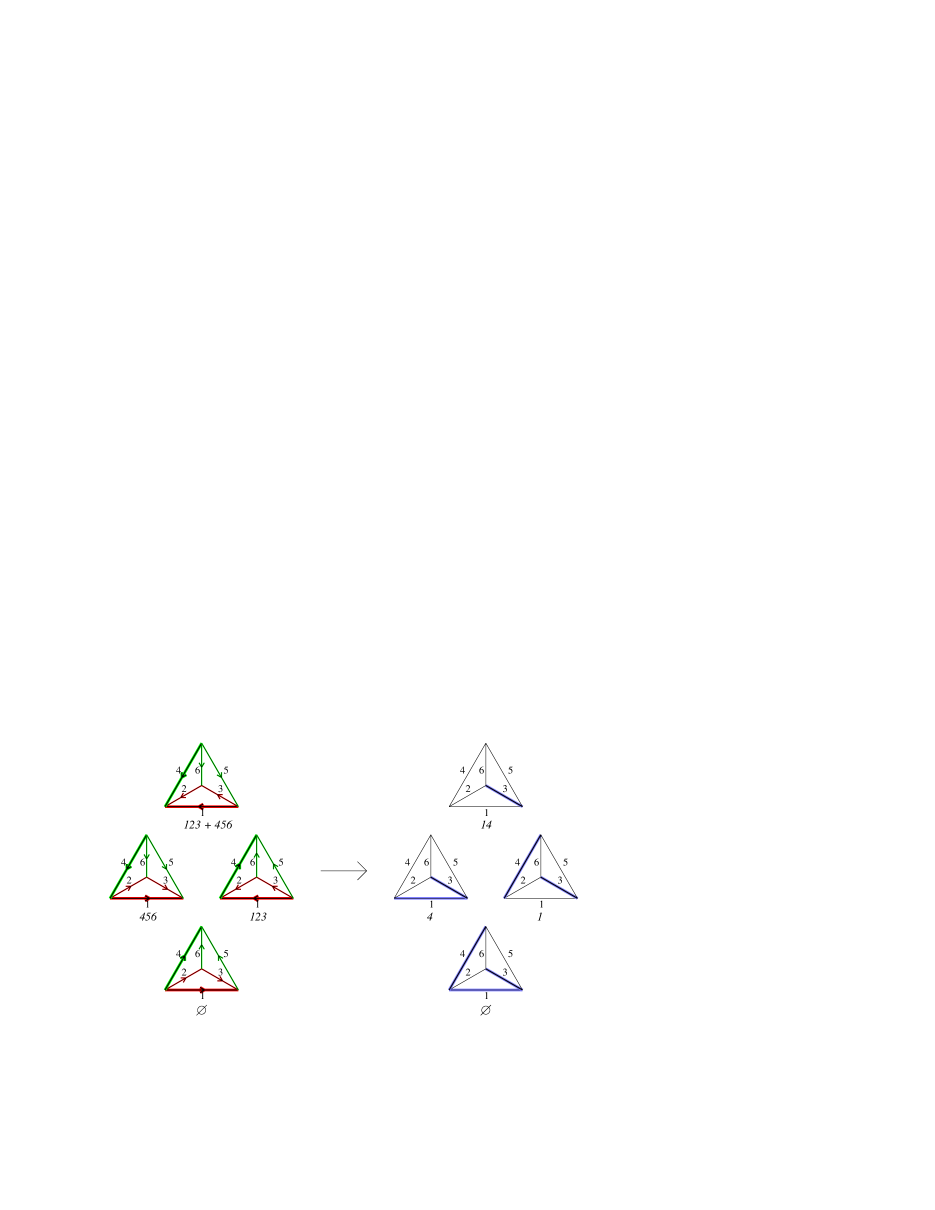
Figure 5: Boolean lattice isomorphism between an activity class of (re)orientations and the interval of the corresponding spanning tree, figured for the class of the graph ${\overrightarrow{G}}$ from Figure 2 with active partition $123+456$ and the spanning tree $T=\alpha({\overrightarrow{G}})$ with $[T\setminus\mathrm{Int}(T),T]=[3,134]$. Edges written below the graphs on the right are those removed from $T$, they correspond to reoriented parts in the digraphs on the left.

Technically, let $G$ be a graph on a linearly ordered set $E$. Let ${\overrightarrow{G}}$ be an orientation of $G$, thought of as the reference orientation. Let $A\subseteq E$. The active partition of $-_{A}{\overrightarrow{G}}$ can be denoted as:

$$E\ =\ \biguplus_{a\ \in\ O(-_{A}{\overrightarrow{G}})\ \cup\ O^{*}(-_{A}{\overrightarrow{G}})}A_{a}$$

where the index of each part is the smallest element of the part. Then, the activity class of $-_{A}{\overrightarrow{G}}$ can be denoted in the following way (where $\triangle$ denotes the symmetric difference):

$$cl(-_{A}{\overrightarrow{G}})=\Biggl{\{}\ -_{A^{\prime}}{\overrightarrow{G}}\ \mid\ A^{\prime}=A\ \triangle\ \Bigl{(}\ \biguplus_{a\in P\cup Q}A_{a}\Bigr{)}\ \text{ for }\ P\subseteq O^{*}(-_{A}{\overrightarrow{G}}),\ Q\subseteq O(-_{A}{\overrightarrow{G}})\ \Biggr{\}}.$$

Let $T=\alpha(-_{A}{\overrightarrow{G}})$ be the active spanning tree of $-_{A}{\overrightarrow{G}}$. The interval of $T$ can be also denoted:

$$[T\setminus\mathrm{Int}(T),T\cup\mathrm{Ext}(T)]\ =\ \Biggl{\{}\ T^{\prime}\subseteq E\ \mid\ T^{\prime}=T\triangle\bigl{(}\biguplus_{a\in P\cup Q}\{a\}\bigr{)}\text{ for }P\subseteq\mathrm{Int}(T),\ Q\subseteq\mathrm{Ext}(T)\ \Biggr{\}}.$$

The above notations emphasize the two boolean lattice structures. Then, we define an isomorphism between the two by choosing that the representative orientation of the activity class which is active-fixed and dual-active fixed w.r.t. ${\overrightarrow{G}}$ (Definition 3.21 and Corollary 3.22) is associated with the spanning tree $T$. Assume $-_{A}{\overrightarrow{G}}$ is the representative of its class with these properties, then we formally have: $\mkern 1.5mu\overline{\mkern-1.5mu\Theta\mkern-1.5mu}\mkern 1.5mu_{\overrightarrow{G}}(A)=O(-_{A}{\overrightarrow{G}})\cap A=\emptyset$ and $\mkern 1.5mu\overline{\mkern-1.5mu\Theta\mkern-1.5mu}\mkern 1.5mu^{*}_{\overrightarrow{G}}(A)=O^{*}(-_{A}{\overrightarrow{G}})\cap A=\emptyset,$ which corresponds to $A^{\prime}=A$, $P=\emptyset$ and $Q=\emptyset$ in the above setting, and which corresponds to the subset $T^{\prime}=T$ in the interval of the spanning tree $T$, that is to $P_{G}(T^{\prime})=\mathrm{Int}(T)\cap T^{\prime}=\emptyset$ and $Q_{G}(T^{\prime})=\mathrm{Ext}(T)\cap T^{\prime}=\emptyset$ (Definitions 3.23 and 2.1). Finally, all orientations in the same activity class and all subsets in the same interval correspond to all possible values of $P$ and $Q$ in the above notations, so that:

$\begin{array}[]{lclclclcl}P&=&\mkern 1.5mu\overline{\mkern-1.5mu\Theta\mkern-1.5mu}\mkern 1.5mu^{*}_{\overrightarrow{G}}(A^{\prime})&=&P_{G}(T^{\prime})&\subseteq&O^{*}(-_{A}{\overrightarrow{G}})&=&\mathrm{Int}(T),\\ Q&=&\mkern 1.5mu\overline{\mkern-1.5mu\Theta\mkern-1.5mu}\mkern 1.5mu_{\overrightarrow{G}}(A^{\prime})&=&Q_{G}(T^{\prime})&\subseteq&O(-_{A}{\overrightarrow{G}})&=&\mathrm{Ext}(T).\end{array}$

By this way, we naturally obtain the following definition and theorem.

Definition 4.40.

Let ${\overrightarrow{G}}$ be a directed graph on a linearly ordered set of edges $E$. For $A\subseteq E$, set

$$\alpha_{\overrightarrow{G}}(A)=\alpha(-_{A}{\overrightarrow{G}})\ \setminus\ \Bigl{(}A\cap O^{*}(-_{A}{\overrightarrow{G}})\Bigr{)}\ \cup\ \Bigl{(}A\cap O(-_{A}{\overrightarrow{G}})\Bigr{)}.$$

In other words, we set $\alpha_{\overrightarrow{G}}(A)=T\setminus P\cup Q$ with $T=\alpha(-_{A}{\overrightarrow{G}}),$ $P=A\cap\mathrm{Int}(T)=A\cap O^{*}(-_{A}{\overrightarrow{G}}),$ and $Q=A\cap\mathrm{Ext}(T)=A\cap O(-_{A}{\overrightarrow{G}}).$ The mapping $\alpha_{\overrightarrow{G}}$ is called the refined active bijection of $G$ w.r.t. ${\overrightarrow{G}}$.

Theorem 4.41.

Let $G$ be a graph on a linearly ordered set of edges $E$, and ${\overrightarrow{G}}$ be an orientation of $G$ (thought of as a reference orientation). We have the following.

• The mapping $-_{A}{\overrightarrow{G}}\mapsto\alpha_{\overrightarrow{G}}(A)$ for $A\subseteq E$ effectively yields a bijection between all reorientations of ${\overrightarrow{G}}$ and all subsets of $E$. It maps activity classes of orientations of $G$ onto intervals of spanning trees of $G$ (and these restrictions are boolean lattice isomophisms).

• For all $A\subseteq E$, $T=\alpha(-_{A}{\overrightarrow{G}})$ and $\alpha_{\overrightarrow{G}}(A)=T\setminus P\cup Q$, we have (with notations of Definitions 3.23 and 2.1):

  $$\mathrm{Int}_{G}(\alpha_{\overrightarrow{G}}(A)) = \scriptstyle\mathrm{Int}_{G}(T)\setminus P \scriptstyle= \scriptstyle O^{*}(-_{A}{\overrightarrow{G}})\setminus P = \Theta^{*}_{\overrightarrow{G}}(A),$$

  $$P_{G}(\alpha_{\overrightarrow{G}}(A)) = \scriptstyle P = \mkern 1.5mu\overline{\mkern-1.5mu\Theta\mkern-1.5mu}\mkern 1.5mu^{*}_{\overrightarrow{G}}(A),$$

  $$\mathrm{Ext}_{G}(\alpha_{\overrightarrow{G}}(A)) = \scriptstyle\mathrm{Ext}_{G}(T)\setminus Q \scriptstyle= \scriptstyle O(-_{A}{\overrightarrow{G}})\setminus Q = \Theta_{\overrightarrow{G}}(A),$$

  $$Q_{G}(\alpha_{\overrightarrow{G}}(A)) = \scriptstyle Q = \mkern 1.5mu\overline{\mkern-1.5mu\Theta\mkern-1.5mu}\mkern 1.5mu_{\overrightarrow{G}}(A).$$

• In particular, $\alpha_{\overrightarrow{G}}(A)$ equals the active spanning tree $\alpha(-_{A}{\overrightarrow{G}})$ if and only if $-_{A}{\overrightarrow{G}}$ is active fixed and dual-active fixed w.r.t. ${\overrightarrow{G}}$. Similarly, restrictions of the mapping $\alpha_{\overrightarrow{G}}$ yield the bijections listed in Table 3.

orientations	subsets	$t(G;2,2)$
acyclic orientations	subsets of internal spanning trees	$t(G;2,0)$
	(or no-broken-circuit subsets)
strongly connected orientations	supersets of external spanning trees	$t(G;0,2)$
dual-active-fixed acyclic orientations	internal spanning trees	$t(G;1,0)$
dual-active-fixed acyclic orientations (w.r.t. $\scriptsize-_{E}{\overrightarrow{G}}$)	min. subsets of internal sp. tree intervals	$t(G;1,0)$
active-fixed strongly connected orientations	external spanning trees	$t(G;0,1)$
active-fixed strongly connected orientations (w.r.t. $\scriptsize-_{\tiny E}{\overrightarrow{G}}$)	max. subsets of external sp. tree intervals	$t(G;0,1)$
active-fixed orientations	subsets of spanning trees	$t(G;2,1)$
	(or forests)
dual-active-fixed orientations	supersets of spanning trees	$t(G;1,2)$
	(or connected spanning subgraphs)
active-fixed and dual-active-fixed orientations	spanning trees	$t(G;1,1)$

Table 3: Remarkable restrictions of the refined active bijection of $G$ w.r.t. $\vec{G}$, between particular types of orientations (first column, in terms of Definition 3.21) and particular types of edge subsets (second column) enumerated by Tutte polynomial evaluations (third column). See Theorem 4.41.

As written above, the refined active bijection of the ordered graph $G$ w.r.t. (the reference reorientation) ${\overrightarrow{G}}$ is the bijection provided by Theorem 4.41. It is important to insist that, in contrast with the canonical one, this bijection is induced by the choice of a reference orientation. Let us mention that the inverse mapping can be computed by a single pass over $E$, see Section 5.2. Let us mention a deletion/contraction construction, see Section 6.3. Lastly, let us mention that variants can be defined, for instance by exchanging the correspondences between the four parameter activities for spanning trees and orientations, see Section 4.4 below.

Proof of Theorem 4.41.

The first point directly comes from the discussion above the theorem. The second point also easily comes from this discussion. Let us precisely check the equalities of parameters in the second point anyway. In order to simplify notations, we omit subscripts ($G$ or ${\overrightarrow{G}}$) of activity parameters. Let $A_{T}$ be the reorientation of ${\overrightarrow{G}}$ whose image under $\alpha_{\overrightarrow{G}}$ is the spanning tree $T$. Let $E=\uplus_{a\in O(-_{A_{T}}{\overrightarrow{G}})\cup O^{*}(-_{A_{T}}{\overrightarrow{G}})}A_{a}$, with $a=\mathrm{min}(A_{a})$, be the active partition associated with $T$ or $-_{A_{T}}{\overrightarrow{G}}$. Let $A$ be a subset in the associated activity class, we have $A=A_{T}\triangle\bigl{(}\cup_{a\in P\cup Q}A_{a}\bigr{)}$ for some $P\subseteq\mathrm{Int}(T)=O^{*}(-_{A_{T}}{\overrightarrow{G}})=O^{*}(-_{A}{\overrightarrow{G}})$ and $Q\subseteq\mathrm{Ext}(T)=O(-_{A_{T}}{\overrightarrow{G}})=O(-_{A}{\overrightarrow{G}})$ with $P\cap A_{T}=\emptyset$ and $Q\cap A_{T}=\emptyset$. By Definition 4.40, we have $\alpha_{\overrightarrow{G}}(A)=T\setminus P\cup Q$ .

By Definition 2.1, we have $\mathrm{Int}(\alpha_{\overrightarrow{G}}(A))=\mathrm{Int}(T)\cap\alpha_{\overrightarrow{G}}(A)$. We have $\mathrm{Int}(T)\cap\alpha_{\overrightarrow{G}}(A)=\mathrm{Int}(T)\cap(T\setminus P\cup Q)=\mathrm{Int}(T)\setminus P$. By Theorem 4.34, we have $\mathrm{Int}(T)\setminus P=O^{*}(-_{A}{\overrightarrow{G}})\setminus P$. By properties of $P$, we have $O^{*}(-_{A}{\overrightarrow{G}})\setminus P=O^{*}(-_{A}{\overrightarrow{G}})\setminus\bigl{(}A_{T}\triangle(\cup_{a\in P\cup Q}A_{a})\bigr{)}=O^{*}(-_{A}{\overrightarrow{G}})\setminus A$. By Definition 3.23, we have $O^{*}(-_{A}{\overrightarrow{G}})\setminus A=\Theta^{*}(A)$. So finally $\mathrm{Int}_{G}(\alpha_{\overrightarrow{G}}(A))=\Theta^{*}(A)$.

On one hand, by Definition 2.1, we have $\mathrm{Int}(\alpha_{\overrightarrow{G}}(A))\cup P(\alpha_{\overrightarrow{G}}(A))=\mathrm{Int}(T)$. On the other hand, by Definition 3.23, we have $\Theta^{*}(A)\cup\mkern 1.5mu\overline{\mkern-1.5mu\Theta\mkern-1.5mu}\mkern 1.5mu^{*}(A)=O^{*}(-_{A}{\overrightarrow{G}})$. By Theorem 4.34, we have $\mathrm{Int}(T)=O^{*}(-_{A}{\overrightarrow{G}})$, so, by the above result, we get $P(\alpha_{\overrightarrow{G}}(A))=\mkern 1.5mu\overline{\mkern-1.5mu\Theta\mkern-1.5mu}\mkern 1.5mu^{*}(A)$.

Similarly, by Definition 2.1, we have $\mathrm{Ext}(\alpha_{\overrightarrow{G}}(A))=\mathrm{Ext}(T)\setminus\alpha_{\overrightarrow{G}}(A)$. We have $\mathrm{Ext}(T)\setminus\alpha_{\overrightarrow{G}}(A)=\mathrm{Ext}(T)\setminus(T\setminus P\cup Q)=\mathrm{Ext}(T)\setminus Q$. By Theorem 4.34, we have $\mathrm{Ext}(T)\setminus Q=O(-_{A}{\overrightarrow{G}})\setminus Q$. As above, by properties of $Q$, we have $O(-_{A}{\overrightarrow{G}})\setminus Q=O(-_{A}{\overrightarrow{G}})\setminus\bigl{(}A_{T}\triangle(\cup_{a\in P\cup Q}A_{a})\bigr{)}=O(-_{A}{\overrightarrow{G}})\setminus A$. As above, by Definition 3.23, we have $O(-_{A}{\overrightarrow{G}})\setminus A=\Theta(A)$. So finally $\mathrm{Ext}(\alpha_{\overrightarrow{G}}(A))=\Theta(A)$. And, as above, we deduce that $Q(\alpha_{\overrightarrow{G}}(A))=\mkern 1.5mu\overline{\mkern-1.5mu\Theta\mkern-1.5mu}\mkern 1.5mu(A)$.

Now, let us consider the list of bijections of the third point. They are all obtained as restrictions of $\alpha_{\overrightarrow{G}}$. Observe that an orientation is active-fixed, resp. dual-active-fixed, if it is obtained by $Q=\emptyset$, resp. $P=\emptyset$. Therefore, all these bijections are obvious by the definitions, except the two ones involving $t(G;1,2)$ and $t(G;2,1)$. For the first one, resp. second one, of these two, we can use that subsets, resp. supersets, of spanning trees are exactly the subsets of type $T\setminus P$, resp. $T\cup Q$, for some spanning tree $T$ and $P\subseteq\mathrm{Int}(T)$, resp. $Q\subseteq\mathrm{Ext}(T)$. This result is stated separately in Lemma 4.42 below. ∎

Lemma 4.42.

Let $G$ be an ordered graph. The set of subsets of spanning trees of $G$ is the union of intervals $[T\setminus\mathrm{Int}_{G}(T),T]$ over all spanning trees $T$ of $G$. The set of supersets of spanning trees of $G$ is the union of intervals $[T,T\cup\mathrm{Ext}_{G}(T)]$ over all spanning trees $T$ of $G$.

Proof.

By the main result of [11] (implying Corollary 3.17, and extended in Theorem 5.43 below), we know that spanning trees $T$ of $G$ are exactly subsets of the form $T_{\iota}\uplus T_{\varepsilon}$ where $T_{\iota}$ is an internal spanning tree of $G/F$, $T_{\varepsilon}$ is an external spanning tree of $G(F)$, and $F$ is a cyclic flat of $G$. Moreover $\mathrm{Int}(T)=\mathrm{Int}_{G/F}(T_{\iota})$ and $\mathrm{Ext}(T)=\mathrm{Ext}_{G(F)}(T_{\varepsilon})$ (for short, we omit these subscripts below).

We have $[T\setminus\mathrm{Int}(T),T\cup\mathrm{Ext}(T)]=[(T_{\iota}\uplus T_{\varepsilon})\setminus\mathrm{Int}(T_{\iota}),(T_{\iota}\uplus T_{\varepsilon})\cup\mathrm{Ext}(T_{\varepsilon})]$. Using the classical partition of $2^{E}$ into spanning tree intervals [9] recalled in the previous discussion, we have:

$\displaystyle 2^{E}=\biguplus_{T\text{ spanning tree}}[T\setminus\mathrm{Int}(T),T\cup\mathrm{Ext}(T)]=\biguplus_{F,\ T_{\iota},\ T_{\varepsilon}\text{ as above}}[T_{\iota}\setminus\mathrm{Int}(T_{\iota}),T_{\iota}]\times[T_{\varepsilon},T_{\varepsilon}\cup\mathrm{Ext}(T_{\varepsilon})]$

(where $\times$ yields all unions of a subset of the first set and a subset of the second set). So we have

$\displaystyle\biguplus_{T\text{ spanning tree}}[T\setminus\mathrm{Int}(T),T]=\biguplus_{F,\ T_{\iota},\ T_{\varepsilon}\text{ as above}}[T_{\iota}\setminus\mathrm{Int}(T_{\iota}),T_{\iota}]\times[T_{\varepsilon}]$

The size of the second set of the equality equals $\sum_{F}t(G/F;2,0)t(G(F);0,1)$ by classical evaluations of the Tutte polynomial. And this number equals $t(G;2,1)$ by the convolution formula (Corollary 3.17), which equals the number of subsets of spanning trees (as well known). The first set of the equality is included in the set of subsets of spanning trees, and it has the same size, hence it equals the set of subsets of spanning trees. Similarly (dually in fact), we get the result involving supersets of spanning trees, whose number equals $t(G;2,1)$. ∎

4.4 A general decomposition framework for classes of activity preserving bijections

Let us briefly observe how the three level construction described in Sections 4.1, 4.2 and 4.3 can be relaxed so as to derive a whole class of active partition preserving mappings (hence also activity preserving), satisfying similar bijective and decomposition properties. Among the bijections of this class, the active bijection is uniquely determined by its canonical construction at the first level, and its natural specification at the third level. What we call preserving is again the transformation of active elements, etc., into their counterpart for orientations/subsets.

First level

Assume that, for any ordered graph $G$, a mapping $\psi_{G}$ provides a bijection between orientations ${\overrightarrow{G}}$ of $G$ which are bipolar, resp. cyclic-bipolar, w.r.t. their smallest edge with fixed orientation, and the spanning trees $\psi_{G}({\overrightarrow{G}})$ of $G$ which are internal, resp. external, uniactive. Assume also that two opposite orientations have the same image (so that the mapping $\psi_{G}$ has the same properties as the uniactive bijection ${\overrightarrow{G}}\mapsto\alpha({\overrightarrow{G}})$ stated in Theorem 4.29).

Second level

From the mappings $\psi_{G}$ available at the first level, one can extend their domains to all orientations of ${\overrightarrow{G}}$, using the same properties as for the canonical active bijection in Definitions 4.30, 4.31 and 4.33. Indeed, as discussed there, the validity and equivalence of these definitions only relies upon properties of the active filtration/partition/minors addressed in Section 3. Precisely, for an ordered digraph ${\overrightarrow{G}}$ with active minors ${\overrightarrow{G}}_{k}$, ${1\leq k\leq\iota}$, in the acyclic part, and ${\overrightarrow{G}}^{\prime}_{k}$, ${1\leq k\leq\varepsilon}$, in the cyclic part, we define

$$\psi_{G}({\overrightarrow{G}})=\ \biguplus_{1\leq k\leq\iota}\psi_{G_{k}}\bigl{(}{\overrightarrow{G}}_{k}\bigr{)}\ \uplus\ \biguplus_{1\leq k\leq\varepsilon}\psi_{G^{\prime}_{k}}\bigl{(}{\overrightarrow{G}}^{\prime}_{k}\bigr{)}.$$

At this step, similarly as for Theorem 4.34, using the bijections at the first level and the decompositions of orientations and spanning trees provided by Theorems 3.14 and 5.43, one can easily check that: $\psi_{G}$ yields an activity preserving, and active partition preserving, bijection between activity classes of orientations and spanning trees of $G$.

Third level

As discussed in Section 4.3, from any bijection $\psi_{G}$ between activity classes of orientations and spanning trees that preserves active elements, one can build a whole class of bijections between orientations and subsets, such that it maps each activity class of orientations onto a spanning tree interval. One can naturally demand that these restrictions are boolean lattice isomorphisms, which can be settled independently of each other. For example, in each restriction, one can demand that the four activity parameters for orientations are transformed into the four activity parameter for subsets, but with possible exchanges in comparison with the refined active bijection (i.e. make $\mathrm{Int}$ correspond to $\mkern 1.5mu\overline{\mkern-1.5mu\Theta\mkern-1.5mu}\mkern 1.5mu^{*}$ instead of $\Theta^{*}$, and/or make $\mathrm{Ext}$ correspond to $\mkern 1.5mu\overline{\mkern-1.5mu\Theta\mkern-1.5mu}\mkern 1.5mu$ instead of $\Theta$). Similarly, one can define active-fixed and dual-active-fixed orientations with respect to two different references orientations respectively, or with respect to variable reference orientations.

Lastly, let us roughly mention that one can also add a deletion/contraction property to the class of mappings considered in this section, yielding the class mentioned in Section 6.3, option 2c (which is thus at the intersection of the classes considered in this section and that one).

5 Counterparts from the spanning tree viewpoint

This section has a special status in the paper. While the above is essentially written from orientations to spanning trees, here we take the inverse viewpoint. We gather results intrinsically involving spanning trees and constructions starting from spanning trees (except subset activities refining spanning tree activities, that have been addressed in Section 2.5).

5.1 The active partition/filtration of a spanning tree - Decomposition of the set of all spanning trees of an ordered graph

First, we give a general decomposition theorem for spanning trees in terms of filtrations of an ordered graph. This theorem refines, at the uniactive level, the decomposition into internal/external spanning trees from [11], where only the cyclic flat $F_{c}$ was involved. It is the counterpart for spanning trees of Theorem 3.14, and it can be derived from this latter theorem and the canonical active bijection (it is generalized to matroid bases in [25], in an intrinsic way, since a proof using orientations is not possible in non-orientable matroids: here we take benefit of graph orientability).

Second, we define the active partition of a spanning tree. This fundamental notion can be defined in multiple ways (it was briefly introduced in [20]). A noticeable feature of the active partition of a spanning tree is that it depends only on the fundamental cycles/cocyles of the spanning tree, but not on the whole graph (in fact, it can be generally seen as a decomposition of a bipartite graph on a linearly ordered set of vertices: edges of the spanning tree are considered as one part of a new set of vertices, the complementary set of edges form the other part, and two vertices are adjacent if they belong to the same fundamental cycle/cocycle). Again, more details and constructions can be found in [25], as well as detailed examples on spanning trees of $K_{4}$ (consistently with Section  7).

Theorem 5.43.

Let $G$ be a graph on a linearly ordered set of edges $E$.

$$\bigl{\{}\ \text{spanning trees of }G\ \bigr{\}}\ \ =\biguplus_{\begin{subarray}{c}\emptyset=F^{\prime}_{\varepsilon}\subset...\subset F^{\prime}_{0}=F_{c}\\[2.84526pt] F_{c}=F_{0}\subset...\subset F_{\iota}=E\\[2.84526pt] \text{\small connected filtration of $\scriptsize G$}\end{subarray}}\Biggl{\{}\ \ T^{\prime}_{1}\uplus...\uplus T^{\prime}_{\varepsilon}\uplus T_{1}\uplus...\uplus T_{\iota}\ \ \mid$$

$$\text{for all }1\leq k\leq\varepsilon,\ T^{\prime}_{k}\hbox{ spanning tree of }G(F^{\prime}_{k-1})/F^{\prime}_{k}\text{ with $|\mathrm{Int}(T^{\prime}_{k})|=0$ and $|\mathrm{Ext}(T^{\prime}_{k})|=1$,}\hphantom{\ \ \Biggr{\}}}$$

$$\text{for all }1\leq k\leq\iota,\ T_{k}\hbox{ spanning tree of }G(F_{k})/F_{k-1}\text{ with $|\mathrm{Int}(T_{k})|=1$ and $|\mathrm{Ext}(T_{k})|=0$}\ \ \Biggr{\}}\hphantom{,}$$

With $T=T^{\prime}_{1}\uplus...\uplus T^{\prime}_{\varepsilon}\uplus T_{1}\uplus...\uplus T_{\iota}$ we then have:

$$\mathrm{Int}(T)\ =\ \uplus_{1\leq k\leq\iota}\mathrm{min}(F_{k}\setminus F_{k-1})\ =\ \uplus_{1\leq k\leq\iota}\mathrm{Int}(T_{k}),$$

$$\mathrm{Ext}(T)\ =\ \uplus_{1\leq k\leq\varepsilon}\mathrm{min}(F^{\prime}_{k-1}\setminus F^{\prime}_{k})\ =\ \uplus_{1\leq k\leq\varepsilon}\mathrm{Ext}(T^{\prime}_{k}).$$

Proof of Theorem 5.43.

This is direct from Theorem 4.34 and Theorem 3.14. More precisely, by Theorem 4.34, a spanning tree $T$ is the image of an orientation ${\overrightarrow{G}}$ by $\alpha$, hence it is a union of uniactive internal/external spanning trees in minors of $G$ induced by the active filtration of ${\overrightarrow{G}}$. Conversely, for any connected filtration of $G$, the uniactive internal/external spanning trees of the minors induced by the sequence are images of some bipolar/cyclic-bipolar minors of an orientation ${\overrightarrow{G}}$, by Theorem 3.14. ∎

From the above result and the constructions of Section 4.2, we can derive the next definition, followed by its multiple equivalent constructions (completed with statements from [20, 25]).

Definition 5.44.

Let $G$ be a graph on a linearly ordered set of edges $E$. Let $T$ be a spanning tree of $G$. The active filtration of $T$ in $G$ is the unique connected filtration of $G$ associated to $T$ in the decomposition given by Theorem 5.43. It is thus the unique filtration $\emptyset=F^{\prime}_{\varepsilon}\subset...\subset F^{\prime}_{0}=F_{c}=F_{0}\subset...\subset F_{\iota}=E$ of $G$ such that:

• for $1\leq k\leq\iota$, $T\cap(F_{k}\setminus F_{k-1})$ is an internal uniactive spanning tree of $G(F_{k})/F_{k-1}$,

• for $1\leq k\leq\varepsilon$, $T\cap(F^{\prime}_{k-1}\setminus F_{k})$ is an external uniactive spanning tree of $G(F^{\prime}_{k-1})/F^{\prime}_{k}$

(such a filtration is necessarily connected, otherwise one of the induced minors has no spanning tree with the required property, see Lemma 3.11). The active partition of $T$ in $G$ is the partition of $E$ formed by successive differences of subsets in the active filtration (yielding parts whose smallest elements are the internally/externally active elements of $T$).

Observation 5.45.

The active filtration/partition of $T$ in $G$ can also be defined as the active filtration/partition of any orientation ${\overrightarrow{G}}$ of $G$ such that $\alpha({\overrightarrow{G}})=T$ (by Theorem 4.34).

Proposition 5.46.

Let $G$ be a graph on a linearly ordered set of edges $E$. Let $T$ be a spanning tree of $G$. The active filtration/partition of $T$ in $G$ can be directly built using only the fundamental cycles/cocycles of $T$ in $G$ and the active closure operator by the following equivalent manners.

• Using the active closure in an inductive way (see Definition 4.37 in Section 4.2).

  Assume either $a=\mathrm{max}(\mathrm{Ext}(T))$, or $a=\mathrm{max}(\mathrm{Int}(T))$. Then, the part of the active partition of $T$ containing $a$ is $\mathrm{acl}(\{a\})$ (by Lemma 4.38). Then, removing the part $\mathrm{acl}(\{a\})$ from the active partition of $T$ yields the active partition of $T\setminus\mathrm{acl}(\{a\})$ in $G/\mathrm{acl}(\{a\})$ if $a=\mathrm{max}(\mathrm{Ext}(T))$, or in $G\setminus\mathrm{acl}(\{a\})$ if $a=\mathrm{max}(\mathrm{Int}(T))$ (this is obvious by Observations 3.13 and 4.32 applied to an orientation ${\overrightarrow{G}}$ such that $\alpha({\overrightarrow{G}})=T$).

• Using the active closure in a direct global way.

  Assume $\mathrm{Int}(T)=\{a_{1},...,a_{\iota}\}_{<}$ and $\mathrm{Ext}(T)=\{a^{\prime}_{1},...,a^{\prime}_{\varepsilon}\}_{<}$. It turns out that the active filtration $\emptyset=F^{\prime}_{\varepsilon}\subset...\subset F^{\prime}_{0}=F_{c}=F_{0}\subset...\subset F_{\iota}=E$ of $T$ satisfies:

  • $F_{c}=\mathrm{acl}(\mathrm{Ext}(T))=E\setminus\mathrm{acl}(\mathrm{Int}(T));$

  • $F_{k}=E\setminus\mathrm{acl}(\{a_{k+1},\dots,a_{\iota}\})$, for every $0\leq k\leq\iota-1$;

  • $F^{\prime}_{k}=\mathrm{acl}(\{a^{\prime}_{k+1},\dots,a^{\prime}_{\varepsilon}\})$, for every $0\leq k\leq\varepsilon-1$.

  This is the definition that was given in [20, Section 5]. The equivalence with the above one is proved in [25] (among various properties and alternative constructions of the active closure).

• Using a linear single pass algorithm over $E$.

  This construction is contained in Theorem 5.50 below, and it is proved in [25] too (by means of a more general single pass construction of the active closure).

5.2 The three levels of the active bijection starting from spanning trees - An all-in-one single-pass construction from spanning trees

Concerning the uniactive bijection addressed in Section 4.1, starting from a uniactive spanning tree, it is obvious to direct the edges one by one so that the criterion of Definitions 4.26 or 4.27 is satisfied. We obtain the next algorithm which works for uniactive internal or external spanning trees as well. See [20, Proposition 3] for details and for two alternative dual formulations, in terms of cycles only or cocycles only. Note that this algorithm consists in a single pass over the edge-set, which is extended to all spanning trees thereafter, whereas the direct computation of $\alpha$ is not easy. This “one way function” feature of the active bijection is noteworthy (see also Section 1 and [29]).

Proposition 5.47 (uniactive bijection from spanning trees, see also [20, Proposition 3]).

Let $G$ be a graph on a linearly ordered set of edges $E=\{e_{1},\dots,e_{n}\}_{<}$. For a spanning tree $T$ with internal activity $1$ and external activity $0$, or internal activity $0$ and external activity $1$, the two opposite orientations of $G$ whose image under $\alpha$ is $T$ are computed by the following algorithm.

Orient $e_{1}$ arbitrarily.

For $k$ from $2$ to $n$ do

if $e_{k}\in T$ then

let $a=\mathrm{min}(C^{*}(T;e_{k}))$

orient $e_{k}$ in order to have $a$ and $e_{k}$ with opposite directions in $C^{*}(T;e_{k})$

if $e_{k}\not\in T$ then

let $a=\mathrm{min}(C(T;e_{k}))$

orient $e_{k}$ in order to have $a$ and $e_{k}$ with opposite directions in $C(T;e_{k})$

The next definition is a direct rephrasing of Definition 4.31, once Theorem 4.34 is acknowledged.

Proposition 5.48 (canonical active bijection from spanning trees).

Let $G$ be an ordered graph. Let $T$ be a spanning tree of $G$, with active filtration $\emptyset=F^{\prime}_{\varepsilon}\subset...\subset F^{\prime}_{0}=F_{c}=F_{0}\subset...\subset F_{\iota}=E$. Let us denote $\alpha_{G}^{-1}(T)$ the set of orientations of $G$ whose image under $\alpha$ is $T$. Then we have:

$$\alpha_{G}^{-1}(T)\ =\ \bigtimes_{1\leq k\leq\iota}\alpha_{G(F_{k})/F_{k-1}}^{-1}(T\cap(F_{k}\setminus F_{k-1}))\ \times\ \bigtimes_{1\leq k\leq\varepsilon}\alpha_{G(F^{\prime}_{k-1})/F^{\prime}_{k}}^{-1}(T\cap(F^{\prime}_{k-1}\setminus F_{k}))\$$

where $\times$ means that the $2^{\iota+\varepsilon}$ resulting orientations of $G$ are inherited from the orientations of the involved minors the natural way (and where each induced spanning tree of a minor is uniactive).∎

The inverse image under the refined active bijection can be directly defined by specifying the orientation within its activity class, as discussed in Section 4.3, and as reformulated below.

Proposition 5.49 (refined active bijection from subsets).

Let $G$ be an ordered graph with reference orientation ${\overrightarrow{G}}$. Let $A$ be a subset in the interval of a spanning tree of $G$ with active filtration $\emptyset=F^{\prime}_{\varepsilon}\subset...\subset F^{\prime}_{0}=F_{c}=F_{0}\subset...\subset F_{\iota}=E$. Then we have:

$$\alpha_{\overrightarrow{G}}^{-1}(A)\ =\ \biguplus_{1\leq k\leq\iota}\alpha_{{\overrightarrow{G}}(F_{k})/F_{k-1}}^{-1}(A\cap(F_{k}\setminus F_{k-1}))\ \uplus\ \biguplus_{1\leq k\leq\varepsilon}\alpha_{{\overrightarrow{G}}(F^{\prime}_{k-1})/F^{\prime}_{k}}^{-1}(A\cap(F^{\prime}_{k-1}\setminus F_{k})).$$

Proof.

This is a straightforward reformulation of the construction of the refined active bijection discussed in Section 4.3. Let us give details anyway. Consider any of the involved minors $H$, and the uniactive spanning tree $T_{H}$ induced in the minor $H$ by the involved spanning tree $T$. The inverse image of $T_{H}$ under $\alpha$ in $H$ consists of two opposite orientations of $H$. Now consider the refined active bijection of $H$ w.r.t. the orientation of $H$ induced by ${\overrightarrow{G}}$, and denote $a$ the smallest edge of $H$. One of the two above orientations is associated to $T_{H}$ (the one for which the orientation of $a$ agrees with ${\overrightarrow{G}}$), and the other to $T_{H}\triangle\{a\}$. Applying this to each minor $H$ and to any subset $A$ in the same interval, we always obtain a reorientation of ${\overrightarrow{G}}$ whose image under $\alpha_{\overrightarrow{G}}$ is $A$. ∎

For completeness of the overview given in this paper, we give below a direct construction from spanning trees/subsets to orientations, using graph terminology. It is stated in [26] for general oriented matroids and the proof essentially relies upon [25] (or also [14]). It combines the inverse computation of fully optimal spanning trees in bipolar minors (Proposition 5.47) with the computation of the active partition from [25]. Noticeably, it uses only the fundamental cycles and cocycles of the spanning tree, not the whole graph structure. The single pass linear algorithm below builds at the same time: the active partition of a spanning tree (Theorem 5.43, refining the partition into internal/external edges from [11]), the premiage of a spanning tree under the canonical active bijection (Theorem 4.34 and Proposition 5.48), and the preimage of a subset under the refined active bijection (Theorem 4.41 and Proposition 5.49).

Theorem 5.50 (all-in-one single-pass algorithm from spanning trees [25, 26]).

Let $G$ be a graph on a linearly ordered set of edges $E=e_{1}<\ldots<e_{n}$. Let $T$ be a spanning tree of $G$.

In the algorithm below, the active partition of $T$ is computed as a mapping, denoted $\mathrm{Part}$, from $E$ to $\mathrm{Int}(T)\cup\mathrm{Ext}(T)$, that maps an edge onto the smallest element of its part in the active partition of $T$. An edge is called internal, resp. external, if its image is in $\mathrm{Int}(T)$, resp. $\mathrm{Ext}(T)$.

The set of $2^{|\mathrm{Int}(T)|+|\mathrm{Ext}(T)|}$ orientations formed by the preimages of $T$ under $\alpha$ in the graph $G$, denoted here $\alpha_{G}^{-1}(T)$, is computed by doing all possible arbitrary choices to orient $e_{k}$ during the algorithm. Equivalently, those preimages under $\alpha$ can also be retrieved from one another since we have

$$\alpha_{G}^{-1}(T)=\{\ A\ \triangle\ \mathrm{Part}^{-1}(P\cup Q)\ \mid\ P\subseteq\mathrm{Int}(T),\ Q\subseteq\mathrm{Ext}(T),\ A\in\alpha_{G}^{-1}(T)\ \}.$$

Let ${\overrightarrow{G}}$ be a reference orientation of $G$, and let $X$ be a subset of $E$. We assume that $X=T\setminus P\cup Q$ with $P\subseteq\mathrm{Int}(T)$ and $Q\subseteq\mathrm{Ext}(T)$, or equivalently that $T=X\setminus Q\cup P$ with $Q=Q_{G}(X)$ and $P=P_{G}(X)$ (see Definition 2.1). We also derive the preimage of $X$ under $\alpha_{\overrightarrow{G}}$.

Input: either a spanning tree $T$ of $G$ alone, or a spanning tree $T$ of $G$ and a subset $X=T\setminus P\cup Q$ in the interval of $T$.

Output: either all orientations of $G$ in $\alpha_{G}^{-1}(T)$, or the reorientation of ${\overrightarrow{G}}$ w.r.t. $\alpha_{\overrightarrow{G}}^{-1}(X)$.

For $k$ from $1$ to $n$ do

if $e_{k}\not\in T$ then

if $e_{k}$ is externally active w.r.t. $T$ then

$e_{k}$ is external, $\mathrm{Part}(e_{k}):=e_{k}$, orient $e_{k}$ either arbitrarily (to compute $\alpha^{-1}(T)$)

or with the same direction as in ${\overrightarrow{G}}$ if and only if $e_{k}\not\in Q$ (to compute $\alpha_{\overrightarrow{G}}^{-1}(X)$)

otherwise

if there exists $c<e_{k}$ internal in $C(T;e_{k})$ then

$e_{k}$ is internal

let $c$ $\in$ $C(T;e_{k})$ with $c<e_{k}$, $c$ internal and $\mathrm{Part}(c)$ the greatest possible

let $\mathrm{Part}(e_{k}):=\mathrm{Part}(c)$

otherwise

$e_{k}$ is external

let $c$ $\in$ $C(T;e_{k})$ with $c<e_{k}$ and $\mathrm{Part}(c)$ the smallest possible

let $\mathrm{Part}(e_{k}):=\mathrm{Part}(c)$

let $a$ be the smallest possible in $C(T;e_{k})$ with $\mathrm{Part}(a)=\mathrm{Part}(e_{k})$

orient $e_{k}$ so that $e_{k}$ and $a$ have opposite directions in $C(T;e_{k})$

if $e_{k}\in T$ then (note: the below rules are dual to the above ones)

if $e_{k}$ is internally active w.r.t. $T$ then

$e_{k}$ is internal, $\mathrm{Part}(e_{k}):=e_{k}$, orient $e_{k}$ either arbitrarily (to compute $\alpha^{-1}(T)$)

or with the same direction as in ${\overrightarrow{G}}$ if and only if $e_{k}\not\in P$ (to compute $\alpha_{\overrightarrow{G}}^{-1}(X)$)

otherwise

it there exists $c<e_{k}$ external in $C^{*}(T;e_{k})$ then

$e_{k}$ is external

let $c$ $\in$ $C^{*}(T;e_{k})$ with $c<e_{k}$, $c$ external and $\mathrm{Part}(c)$ the greatest possible

let $\mathrm{Part}(e_{k}):=\mathrm{Part}(c)$

otherwise

$e_{k}$ is internal

let $c$ $\in$ $C^{*}(T;e_{k})$ with $c<e_{k}$ and $\mathrm{Part}(c)$ the smallest possible

let $\mathrm{Part}(e_{k}):=\mathrm{Part}(c)$

let $a$ be the smallest possible in $C^{*}(T;e_{k})$ with $\mathrm{Part}(a)=\mathrm{Part}(e_{k})$

orient $e_{k}$ so that $e_{k}$ and $a$ have opposite directions in $C^{*}(T;e_{k})$

6 Constructions by deletion/contraction

We address deletion/contraction constructions for the three levels of the active bijection. As we will show, in contrast with the previous constructions, these constructions can be thought of as building the whole bijections at once, roughly said as $1-1$ correspondences between orientations and spanning trees/subsets rather than as pairs of inverse mappings from one side to the other. We state these inductive constructions the simplest way, so that they are directly related to what precedes in this paper. This whole section is generalized and developed further in [28], notably with more practical conditions equivalent to the ones used in the following algorithms. At the end, we also present how these constructions fit in a general deletion/contraction framework for building correspondences/bijections involving graduated activity preservation constraints, amongst which the active bijection is uniquely determined by its canonical or natural properties.

6.1 The uniactive bijection

This section repeats results and condenses remarks from the companion paper [29, Section LABEL:ABG2LP-sec:induction].

Lemma 6.51.

Let ${\overrightarrow{G}}$ be a digraph, on a linearly ordered set of edges $E$, which is bipolar w.r.t. $p=\mathrm{min}(E)$. Let $\omega$ be the greatest element of $E$. Let $T=\alpha({\overrightarrow{G}})$. If $\omega\in T$ then ${\overrightarrow{G}}/\omega$ is bipolar w.r.t. $p$ and $T\setminus\{\omega\}=\alpha({\overrightarrow{G}}/\omega)$. If $\omega\not\in T$ then ${\overrightarrow{G}}\backslash\omega$ is bipolar w.r.t. $p$ and $T=\alpha({\overrightarrow{G}}\backslash\omega)$. In particular, we get that ${\overrightarrow{G}}/\omega$ is bipolar w.r.t. $p$ or ${\overrightarrow{G}}\backslash\omega$ is bipolar w.r.t. $p$.

Proof.

First, let us recall that if a spanning tree of a directed graph satisfies the criterion of Definition 4.26, then this directed graph is necessarily bipolar w.r.t. its smallest edge. This is implied by [20, Propositions 2 and 3], or also stated explicitly in [24, Proposition 3.2], and this is easy to see: if the criterion is satisfied, then the spanning tree is internal uniactive (by definitions of internal/external activities) and the digraph is determined up to reversing all edges (see Proposition 5.47), which implies that the digraph is in the inverse image of $T$ by the uniactive bijection of Theorem 4.29 and that it is bipolar w.r.t. its smallest edge.

Assume that $\omega\in T$. Obviously, the fundamental cocycle of $b\in T\setminus\{\omega\}$ w.r.t. $T\setminus\{\omega\}$ in $G/\omega$ is the same as the fundamental cocycle of $b$ w.r.t. $T$ in $G$. And the fundamental cycle of $e\not\in T$ w.r.t. $T\setminus\{\omega\}$ in $G/\omega$ is obtained by removing $\omega$ from the fundamental cycle of $e$ w.r.t. $T$ in $G$. Hence, those fundamental cycles and cocycles in $G/\omega$ satisfy the criterion of Definition 4.26, hence ${\overrightarrow{G}}/\omega$ is bipolar w.r.t. $p$ and $T\setminus\{\omega\}=\alpha({\overrightarrow{G}}/\omega)$.

Similarly (dually in fact), assume that $\omega\not\in T$. The fundamental cocycle of $b\in T$ w.r.t. $T\setminus\{\omega\}$ in $G\backslash\omega$ is obtained by removing $\omega$ from the fundamental cocycle of $b$ w.r.t. $T$ in $G$. And the fundamental cycle of $e\not\in T\setminus\{\omega\}$ w.r.t. $T\setminus\{\omega\}$ in $G\backslash\omega$ is the same as the fundamental cycle of $e$ w.r.t. $T$ in $G$. Hence, those fundamental cycles and cocycles in $G\backslash\omega$ satisfy the criterion of Definition 4.26, hence ${\overrightarrow{G}}\backslash\omega$ is bipolar w.r.t. $p$ and $T\setminus\{\omega\}=\alpha({\overrightarrow{G}}\backslash\omega)$.

Note that the fact that either ${\overrightarrow{G}}/\omega$ is bipolar w.r.t. $p$, or ${\overrightarrow{G}}\backslash\omega$ is bipolar w.r.t. $p$ could also easily be directly proved in terms of digraph properties. ∎

Theorem 6.52.

The fully optimal (or active) spanning trees of ordered bipolar digraphs satisfy the following inductive definition.

For any ordered digraph ${\overrightarrow{G}}$ on $E$, bipolar w.r.t. $p=\mathrm{min}(E)$, and with $\mathrm{max}(E)=\omega$.

If $|E|=1$ then $\alpha({\overrightarrow{G}})=\omega$.

If $|E|>1$ then:

If ${\overrightarrow{G}}/\omega$ is bipolar w.r.t. $p$ but not ${\overrightarrow{G}}\backslash\omega$ then $\alpha({\overrightarrow{G}})=\alpha({\overrightarrow{G}}/\omega)\cup\{\omega\}$.

If ${\overrightarrow{G}}\backslash\omega$ is bipolar w.r.t. $p$ but not ${\overrightarrow{G}}/\omega$ then $\alpha({\overrightarrow{G}})=\alpha({\overrightarrow{G}}\backslash\omega)$.

If both ${\overrightarrow{G}}\backslash\omega$ and ${\overrightarrow{G}}/\omega$ are bipolar w.r.t. $p$ then:

let $T^{\prime}=\alpha({\overrightarrow{G}}\backslash\omega)$, $C=C_{\overrightarrow{G}}(T^{\prime};\omega)$ and $e=\mathrm{min}(C)$

if $e$ and $\omega$ have opposite directions in $C$ then $\alpha({\overrightarrow{G}})=\alpha({\overrightarrow{G}}\backslash\omega)$;

if $e$ and $\omega$ have the same directions in $C$ then $\alpha({\overrightarrow{G}})=\alpha({\overrightarrow{G}}/\omega)\cup\{\omega\}$.

or equivalently:

let $T^{\prime\prime}=\alpha({\overrightarrow{G}}/\omega)$, $D=C^{*}_{\overrightarrow{G}}(T^{\prime\prime}\cup\omega;\omega)$ and $e=\mathrm{min}(D)$

if $e$ and $\omega$ have opposite directions in $D$ then $\alpha({\overrightarrow{G}})=\alpha({\overrightarrow{G}}/\omega)\cup\{\omega\}$;

if $e$ and $\omega$ have the same directions in $D$ then $\alpha({\overrightarrow{G}})=\alpha({\overrightarrow{G}}\backslash\omega)$.

Proof.

By Lemma 6.51, at least one minor among $\{{\overrightarrow{G}}/\omega,{\overrightarrow{G}}\backslash\omega\}$ is bipolar w.r.t. $p$. If exactly one minor among $\{{\overrightarrow{G}}/\omega,{\overrightarrow{G}}\backslash\omega\}$ is bipolar w.r.t. $p$, then by Lemma 6.51 again, the above definition is implied. Assume now that both minors are bipolar w.r.t. $p$.

Consider $T^{\prime}=\alpha({\overrightarrow{G}}\backslash\omega)$. Fundamental cocycles of elements in $T^{\prime}$ w.r.t. $T^{\prime}$ in ${\overrightarrow{G}}$ are obtained by removing $\omega$ from those in ${\overrightarrow{G}}\backslash\omega$. Hence they satisfy the criterion of Definition 4.26. Fundamental cycles of elements in $E\setminus(T^{\prime}\cup\{\omega\})$ w.r.t. $T^{\prime}$ in ${\overrightarrow{G}}$ are the same as in ${\overrightarrow{G}}\backslash\omega$. Hence they satisfy the criterion of Definition 4.26. Let $C$ be the fundamental cycle of $\omega$ w.r.t. $T^{\prime}$. If $e$ and $\omega$ have opposite directions in $C$, then $C$ satisfies the criterion of Definition 4.26, and $\alpha({\overrightarrow{G}})=T^{\prime}$. Otherwise, we have $\alpha({\overrightarrow{G}})\not=T^{\prime}$, and, by Lemma 6.51, we must have $\alpha({\overrightarrow{G}})=\alpha({\overrightarrow{G}}/\omega)\cup\{\omega\}$.

The second condition involving $T^{\prime\prime}=\alpha({\overrightarrow{G}}/\omega)$ is proved in the same manner. Since it yields the same mapping $\alpha$, then this second condition is actually equivalent to the first one, and so it can be used as an alternative. Note that the fact that these two conditions are equivalent is difficult and proved here in an indirect way (actually this fact is equivalent to the key result that $\alpha$ yields a bijection), see [29, Remark LABEL:ABG2LP-rk:ind-10-equivalence]. ∎

Corollary 6.53.

We use notations of Theorem 6.52. If $-_{\omega}{\overrightarrow{G}}$ is bipolar w.r.t. $p$ then the above algorithm of Theorem 6.52 builds at the same time $\alpha({\overrightarrow{G}})$ and $\alpha(-_{\omega}{\overrightarrow{G}})$, we have:

$$\Bigl{\{}\ \alpha({\overrightarrow{G}}),\ \alpha(-_{\omega}{\overrightarrow{G}})\ \Bigr{\}}\ =\ \Bigl{\{}\ \alpha({\overrightarrow{G}}\backslash\omega),\ \alpha({\overrightarrow{G}}/\omega)\cup\{\omega\}\ \Bigr{\}}.$$

Also, we have that $-_{\omega}{\overrightarrow{G}}$ is bipolar w.r.t. $p$ if and only if ${\overrightarrow{G}}\backslash\omega$ and ${\overrightarrow{G}}/\omega$ are bipolar w.r.t. $p$.

Proof.

Direct by Theorem 6.52 and Theorem 4.29 (bijection property). ∎

Important remarks on the above results are given in [29, Section LABEL:ABG2LP-sec:induction]. Let us resituate them here.

Remark 6.54 (equivalence in Theorem 6.52).

The equivalence of the two formulations in the algorithm of Theorem 6.52 is a deep and difficult result, which we directly derive from the bijection provided by the Key Theorem 4.29. Actually, if one defines a mapping $\alpha$ from scratch as in the algorithm (with either one of the two formulations) and then investigates its properties, then it turns out that the above equivalence result is equivalent to the existence and uniqueness of the fully optimal spanning tree (Definition 4.26) and hence to this key theorem. See [28] for precisions.

Furthermore, this equivalence result is also related to the active duality property addressed in Section 4.1. First, recall that cyclic-bipolar orientations of $G$ w.r.t. $p$ with fixed orientation for $p$ are also in bijection with external uniactive spanning trees of $G$. Thanks to the equivalence of these two dual formulations, one can directly adapt the above algorithm for this second bijection, with no risk of inconsistency. Second, let us mention that, as well as the active duality property is a strengthening of linear programming duality, the deletion/contraction algorithm of Theorem 6.52 corresponds to a refinement of the classical linear programming solving by constraint/variable deletion, see [19, 27]. In these terms, and in oriented matroid terms as well, the above equivalence result means that the same algorithm can be equally used in the dual, with no risk of inconsistency.

Remark 6.55 (computational complexity).

Using the construction of Theorem 6.52 to build one single image under $\alpha$ involves an exponential number of images of minors, see details in [29, Remark LABEL:ABG2LP-rk:difficult]. However, this algorithm is efficient for building the images of all bipolar orientations of $G$ at once, in the sense that, with $|E|=n$, the number of calls to the algorithm to build these $O(2^{n})$ images is $O(n.2^{n})$. See details in [29, Remark LABEL:ABG2LP-rk:ind-10], and see Remark 6.56 below. An efficent algorithm for building one single image, involving just one minor for each edge of the resulting spanning tree, is the main result of [29].

Remark 6.56 (building the whole bijection at once, and the CHOICE notion).

By Corollary 6.53, the construction of Theorem 6.52 can be used to build the whole active bijection for $G$ (i.e. the $1-1$ correspondence, or the matching, between all bipolar orientations of $G$ w.r.t. $p$ with fixed orientation, and all internal uniactive spanning trees of $G$), from the whole active bijections for $G/\omega$ and $G\backslash\omega$. For each pair of bipolar orientations $\{{\overrightarrow{G}},-_{\omega}{\overrightarrow{G}}\}$, the algorithm provides which “local choice” is right to associate one orientation with the orientation induced in $G/\omega$ and the other with the orientation induced in $G\setminus\omega$. This CHOICE notion is extended to the general active bijection in Remark 6.60 and it is formally developed in Section 6 (and in [28]) as the basic component for a deletion/contraction framework.

6.2 The canonical active bijection

In this overview paper, we choose to give an inductive definition of the active bijection as concise as possible (based on definitions and proofs from the previous sections), but we point out that the algorithm below can be detailed further as a more practical algorithm in several ways, see Remark 6.62. In the next proposition, we use the properties of $\alpha$ to derive the minimum inductive properties of active partitions required to derive an inductive definition of $\alpha$. More involved and intrinsic inductive properties of active partitions are given and used in [28]. Also, a short alternative formulation in the acyclic case is given in [21].

We call removing the greatest element of $E$ from an active partition of $E$ the natural operation that consists in removing this element from its part in the active partition (and from the associated cyclic flat if it contains it), yielding another partition of $E$.

Proposition 6.57.

Let ${\overrightarrow{G}}$ be a digraph, on a linearly ordered set of edges $E$. Let $\omega$ be the greatest element of $E$. Assume $\omega$ is not an isthmus nor a loop of $G$.

1. We have

   $$\Bigl{\{}\ \alpha({\overrightarrow{G}}),\ \alpha(-_{\omega}{\overrightarrow{G}})\ \Bigr{\}}\ =\ \Bigl{\{}\ \alpha({\overrightarrow{G}}\backslash\omega),\ \alpha({\overrightarrow{G}}/\omega)\cup\{\omega\}\ \Bigr{\}}.$$

2. Moreover, if $\alpha({\overrightarrow{G}})=\alpha({\overrightarrow{G}}\backslash\omega)$, resp. $\alpha({\overrightarrow{G}})=\alpha({\overrightarrow{G}}/\omega)\cup\{\omega\}$, then removing $\omega$ from the active partition of ${\overrightarrow{G}}$ yields the active partition of ${\overrightarrow{G}}\backslash\omega$, resp. ${\overrightarrow{G}}/\omega$.

3. In particular, removing $\omega$ from the active partition of ${\overrightarrow{G}}$ yields either the active partition of ${\overrightarrow{G}}/\omega$ or that of ${\overrightarrow{G}}\backslash\omega$.

4. Moreover, ${\overrightarrow{G}}\backslash\omega$ and ${\overrightarrow{G}}/\omega$ have the same active partition if and only if ${\overrightarrow{G}}$ and $-_{\omega}{\overrightarrow{G}}$ have the same active partition.

Proof.

In what follows, bipolar and cyclic-bipolar are always meant w.r.t. the smallest edge. Moreover, we will consider the bipolar or cyclic-bipolar active minors induced by the active partition of ${\overrightarrow{G}}$ (Proposition 3.12), and denote ${\overrightarrow{G}}_{\omega}$ the minor containing $\omega$ among them, with edge set $E_{\omega}$.

First, we prove (3). Let us prove that removing $\omega$ from the active partition of ${\overrightarrow{G}}$ yields either the active partition of ${\overrightarrow{G}}/\omega$ or that of ${\overrightarrow{G}}\backslash\omega$. By Lemma 6.51 (or by a direct easy proof), we have that ${\overrightarrow{G}}_{\omega}/\omega$ or ${\overrightarrow{G}}_{\omega}\backslash\omega$ is bipolar or cyclic-bipolar (if ${\overrightarrow{G}}_{\omega}$ is cyclic-bipolar, then apply the lemma to $-_{\omega}{\overrightarrow{G}}_{\omega}$ which is bipolar, as recalled in Section 2). Replacing ${\overrightarrow{G}}_{\omega}$ by this minor in the sequence of minors associated with ${\overrightarrow{G}}$ yields the sequence of minors induced by the partition of $E$ obtained by removing $\omega$ from $E_{\omega}$. This partition obviously corresponds to a filtration of $G\backslash\omega$ or $G/\omega$, and its induced minors are either bipolar or cyclic-bipolar (with no change of nature w.r.t. the minors given by the active partition of ${\overrightarrow{G}}$). Hence, by Proposition 3.12, it is necessarily the active partition of $G\backslash\omega$ or $G/\omega$.

Now, we prove (1) and (2). Let us prove that $\alpha({\overrightarrow{G}})\in\bigl{\{}\alpha({\overrightarrow{G}}\backslash\omega),\alpha({\overrightarrow{G}}/\omega)\cup\{\omega\}\bigr{\}}.$ The minor ${\overrightarrow{G}}_{\omega}$ is either bipolar or cyclic-bipolar. In what follows, we can assume that it is bipolar. If it is cyclic-bipolar, then the same reasoning holds, up to applying it to $-_{\omega}{\overrightarrow{G}}_{\omega}$ which is bipolar (see Section 2), and using Definition 4.28 which ensures the compatibility of $\alpha$ with this canonical bijection between bipolar and cyclic-bipolar orientations. We leave the details. By Definition 4.31, we have $\alpha({\overrightarrow{G}})=A\uplus\alpha({\overrightarrow{G}}_{\omega})$ for some $A\subseteq E$.

Assume that removing $\omega$ from the active partition of ${\overrightarrow{G}}$ yields the active partition of ${\overrightarrow{G}}\backslash\omega$. By assumption, we have that ${\overrightarrow{G}}_{\omega}\backslash\omega$ is bipolar. By Definition 4.31, we have $\alpha({\overrightarrow{G}}\backslash\omega)=A\uplus\alpha({\overrightarrow{G}}_{\omega}\backslash\omega)$ since the other minors induced by the active partition of ${\overrightarrow{G}}$ are unchanged by assumption, which implies that $A$ is also unchanged. If $\alpha({\overrightarrow{G}}_{\omega})=\alpha({\overrightarrow{G}}_{\omega}\backslash\omega)$ then $\alpha({\overrightarrow{G}})=\alpha({\overrightarrow{G}}\backslash\omega)$.

Assume now that $\alpha({\overrightarrow{G}}_{\omega})\not=\alpha({\overrightarrow{G}}_{\omega}\backslash\omega)$. Then, by Theorem 6.52, we have that ${\overrightarrow{G}}_{\omega}/\omega$ is bipolar and $\alpha({\overrightarrow{G}}_{\omega})=\alpha({\overrightarrow{G}}_{\omega}/\omega)\cup\{\omega\}$. Since the other minors induced by the active partition of ${\overrightarrow{G}}$ are unchanged by removing $\omega$, we get (as in the first paragraph) that removing $\omega$ from the active partition of ${\overrightarrow{G}}$ also yields the active partition of ${\overrightarrow{G}}/\omega$. Hence $\alpha({\overrightarrow{G}}/\omega)=A\uplus\alpha({\overrightarrow{G}}_{\omega}/\omega)$. Hence $\alpha({\overrightarrow{G}})=\alpha({\overrightarrow{G}}/\omega)\cup\{\omega\}$.

We have proved $\alpha({\overrightarrow{G}})\in\bigl{\{}\alpha({\overrightarrow{G}}\backslash\omega),\alpha({\overrightarrow{G}}/\omega)\cup\{\omega\}\bigr{\}}$. Notice that we have proved in the meantime: if $\alpha({\overrightarrow{G}})=\alpha({\overrightarrow{G}}/\omega))\cup\{\omega\}$ and removing $\omega$ from the active partition of ${\overrightarrow{G}}$ yields the active partition of ${\overrightarrow{G}}\backslash\omega$, then removing $\omega$ from the active partition of ${\overrightarrow{G}}$ also yields the active partition of ${\overrightarrow{G}}/\omega$. So, in every case, we have: if $\alpha({\overrightarrow{G}})=\alpha({\overrightarrow{G}}/\omega)\cup\{\omega\}$ then removing $\omega$ from the active partition of ${\overrightarrow{G}}$ yields the active partition of ${\overrightarrow{G}}/\omega$. A similar reasoning holds if $\alpha({\overrightarrow{G}})=\alpha({\overrightarrow{G}}\backslash\omega)$.

Now, by symmetry, we have proved also $\alpha(-_{\omega}{\overrightarrow{G}})\in\bigl{\{}\alpha({\overrightarrow{G}}\backslash\omega),\alpha({\overrightarrow{G}}/\omega)\cup\{\omega\}\bigr{\}}$. We prove that $\alpha({\overrightarrow{G}})\not=\alpha(-_{\omega}{\overrightarrow{G}})$. Otherwise, ${\overrightarrow{G}}$ and $-_{\omega}{\overrightarrow{G}}$ belong to the same activity class (Definition 3.19), implying that $\omega$ is the unique element of its part in the active partition of ${\overrightarrow{G}}$, implying that $\omega$ is an isthmus or a loop, which is forbidden by hypothesis. So we have $\{\ \alpha({\overrightarrow{G}}),\ \alpha(-_{\omega}{\overrightarrow{G}})\ \}\ =\ \{\ \alpha({\overrightarrow{G}}\backslash\omega),\ \alpha({\overrightarrow{G}}/\omega)\cup\{\omega\}\ \}.$

Now, we prove (4). Assume that ${\overrightarrow{G}}$ and $-_{\omega}{\overrightarrow{G}}$ have the same active partition. Then, obviously, by (1) and (2), removing $\omega$ from this active partition yields the active partition of ${\overrightarrow{G}}\backslash\omega$ and also the active partition of ${\overrightarrow{G}}/\omega$, and so these two active partitions are also equal.

Finally, assume that ${\overrightarrow{G}}\backslash\omega$ and ${\overrightarrow{G}}/\omega$ have the same active partition. Assume that removing $\omega$ from the active partition of ${\overrightarrow{G}}$ yields the common active partition of ${\overrightarrow{G}}\backslash\omega$ and ${\overrightarrow{G}}/\omega$. Assume that ${\overrightarrow{G}}_{\omega}$ is bipolar. Then ${\overrightarrow{G}}_{\omega}\backslash\omega$ is defined on the edge set $E_{\omega}\setminus\{\omega\}$, and, by Proposition 3.12, it is a bipolar minor associated with the active partition of ${\overrightarrow{G}}\backslash\omega$ (the other minors are unchanged, as in the first paragraph). In the same manner, ${\overrightarrow{G}}_{\omega}/\omega$ is a bipolar minor as it is associated with the active partition of ${\overrightarrow{G}}/\omega$. By Corollary 6.53, we then have that $-_{\omega}{\overrightarrow{G}}_{\omega}$ is also bipolar. Hence the active partition of ${\overrightarrow{G}}$ satisfies the characterization given by Proposition 3.12 for the active partition of $-_{\omega}{\overrightarrow{G}}$, and so ${\overrightarrow{G}}$ and $-_{\omega}{\overrightarrow{G}}$ have the same active partition (that is: $-_{\omega}{\overrightarrow{G}}_{\omega}$ is the minor containing $\omega$ associated with the active partition of $-_{\omega}{\overrightarrow{G}}$).

If ${\overrightarrow{G}}_{\omega}$ is cyclic-bipolar, then the same reasoning as above holds. We recall that the active partition is given with the information on the associated cyclic flat, that is on the bipolar or cyclic-bipolar nature of each minor, hence in this case we have that both ${\overrightarrow{G}}_{\omega}\backslash\omega$ and ${\overrightarrow{G}}_{\omega}/\omega$ are cyclic-bipolar. We end the same way up to reversing $\omega$ and using the canonical bijection between bipolar and cyclic-bipolar orientations. So, finally, ${\overrightarrow{G}}$ and $-_{\omega}{\overrightarrow{G}}$ have the same active partition. ∎

Theorem 6.58.

The active spanning trees of ordered digraphs satisfy the following inductive definition.

For any ordered digraph ${\overrightarrow{G}}$ on edge-set $E$, and with $\mathrm{max}(E)=\omega$.

If $E=\emptyset$ then $\alpha({\overrightarrow{G}})=\emptyset$.

(isthmus/loop case)

If $\omega$ is an isthmus of $G$ then $\alpha({\overrightarrow{G}})=\alpha(-_{\omega}{\overrightarrow{G}})=\alpha({\overrightarrow{G}}/\omega)\cup\{\omega\}$.

If $\omega$ is a loop of $G$ then $\alpha({\overrightarrow{G}})=\alpha(-_{\omega}{\overrightarrow{G}})=\alpha({\overrightarrow{G}}\backslash\omega)$.

If $\omega$ is not an isthmus nor a loop of $G$ then:

(choice by activity comparison)

If ${\overrightarrow{G}}/\omega$ and ${\overrightarrow{G}}\backslash\omega$ do not have the same active partition, then let ${\overrightarrow{G}}_{0}$ be the unique minor within $\{{\overrightarrow{G}}/\omega,{\overrightarrow{G}}\backslash\omega\}$ such that the active partition of ${\overrightarrow{G}}_{0}$ is obtained by removing $\omega$ from the active partition of ${\overrightarrow{G}}$ (well-defined by Proposition 6.57 (2)).

If ${\overrightarrow{G}}/\omega$ and ${\overrightarrow{G}}\backslash\omega$ have the same active partition, then let ${\overrightarrow{G}}_{\omega}$ be the minor containing $\omega$ associated with the active partition of ${\overrightarrow{G}}$ on set of edges $E_{\omega}$, and then:

(choice by full optimality)

let $T^{\prime}=\alpha({\overrightarrow{G}}_{\omega}\backslash\omega)=\alpha({\overrightarrow{G}}\backslash\omega)\cap E_{\omega}$, $C=C_{{\overrightarrow{G}}_{\omega}}(T^{\prime};\omega)$ and $e=\mathrm{min}(C)$

if $e$ and $\omega$ have opposite directions in $C$ then let ${\overrightarrow{G}}_{0}={\overrightarrow{G}}\backslash\omega$

if $e$ and $\omega$ have the same directions in $C$ then let ${\overrightarrow{G}}_{0}={\overrightarrow{G}}/\omega$

or equivalently:

let $T^{\prime\prime}=\alpha({\overrightarrow{G}}_{\omega}/\omega)=\alpha({\overrightarrow{G}}/\omega)\cap E_{\omega}$, $D=C^{*}_{{\overrightarrow{G}}_{\omega}}(T^{\prime\prime}\cup\omega;\omega)$ and $e=\mathrm{min}(D)$

if $e$ and $\omega$ have opposite directions in $D$ then let ${\overrightarrow{G}}_{0}={\overrightarrow{G}}/\omega$

if $e$ and $\omega$ have the same directions in $D$ then let ${\overrightarrow{G}}_{0}={\overrightarrow{G}}\backslash\omega$.

(assignment step)

If ${\overrightarrow{G}}_{0}={\overrightarrow{G}}\backslash\omega$	then	$\alpha({\overrightarrow{G}})=\alpha({\overrightarrow{G}}\backslash\omega)$	and	$\alpha(-_{\omega}{\overrightarrow{G}})=\alpha({\overrightarrow{G}}/\omega)\cup\{\omega\}$.
If ${\overrightarrow{G}}_{0}={\overrightarrow{G}}/\omega$	then	$\alpha({\overrightarrow{G}})=\alpha({\overrightarrow{G}}/\omega)\cup\{\omega\}$	and	$\alpha(-_{\omega}{\overrightarrow{G}})=\alpha({\overrightarrow{G}}\backslash\omega)$.

Let us recall that, with notations used in Theorem 6.58, ${\overrightarrow{G}}_{\omega}$ bipolar, resp. cyclic-bipolar, if and only if $\omega$ belongs to a directed cocycle, resp. directed cycle, of ${\overrightarrow{G}}$.

Proof.

We follow the cases addressed during the algorithm and we prove that, in every case, the resulting definition of $\alpha$ is correct. If $\omega$ is an isthmus or a loop, then $\omega$ is the only element of its part in the active partition of ${\overrightarrow{G}}$, and then the definition is obviously correct as it coincides with Definition 4.31. Assume now that $\omega$ is not an isthmus nor a loop.

Assume ${\overrightarrow{G}}/\omega$ and ${\overrightarrow{G}}\backslash\omega$ do not have the same active partition. By Proposition 6.57, the active partition of at least one of the two minors in $\{{\overrightarrow{G}}/\omega,{\overrightarrow{G}}\backslash\omega\}$ is obtained by removing $\omega$ from the active partition of $\omega$. Hence ${\overrightarrow{G}}_{0}$ is well defined. Assume ${\overrightarrow{G}}_{0}={\overrightarrow{G}}\backslash\omega$. By Proposition 6.57, we have $\alpha({\overrightarrow{G}})\in\bigl{\{}\alpha({\overrightarrow{G}}\backslash\omega),\alpha({\overrightarrow{G}}/\omega)\cup\{\omega\}\bigr{\}}$. Moreover, if $\alpha({\overrightarrow{G}})=\alpha({\overrightarrow{G}}/\omega)\cup\{\omega\}$ then removing $\omega$ from the active partition of ${\overrightarrow{G}}$ yields the active partition of ${\overrightarrow{G}}/\omega$, which contradicts the definition of ${\overrightarrow{G}}_{0}$. Hence $\alpha({\overrightarrow{G}})=\alpha({\overrightarrow{G}}\backslash\omega)$. And hence, by Proposition 6.57, we also have $\alpha(-_{\omega}{\overrightarrow{G}})=\alpha({\overrightarrow{G}}/\omega)\cup\{\omega\}$. So the definition given in the theorem is correct (the same reasoning holds for ${\overrightarrow{G}}_{0}={\overrightarrow{G}}/\omega$).

Assume now that ${\overrightarrow{G}}/\omega$ and ${\overrightarrow{G}}\backslash\omega$ have the same active partition. By Proposition 6.57, we have at the same time that ${\overrightarrow{G}}_{\omega}$ is the minor containing $\omega$ associated with the active partition of ${\overrightarrow{G}}$, and that $-_{\omega}{\overrightarrow{G}}_{\omega}$ is the minor containing $\omega$ associated with the active partition of $-_{\omega}{\overrightarrow{G}}$. And since we have $\alpha({\overrightarrow{G}}\backslash\omega)\in\{\alpha({\overrightarrow{G}}),\alpha(-_{\omega}{\overrightarrow{G}})\}$, then we have (by Definition 4.31) $\alpha({\overrightarrow{G}}_{\omega}\backslash\omega)=\alpha({\overrightarrow{G}}\backslash\omega)\cap E_{\omega}$. Similarly, we have $\alpha({\overrightarrow{G}}_{\omega}/\omega)=\alpha({\overrightarrow{G}}/\omega)\cap E_{\omega}$.

If ${\overrightarrow{G}}_{\omega}\backslash\omega$ (or equivalently ${\overrightarrow{G}}_{\omega}/\omega$) is bipolar w.r.t. its smallest edge, then the two equivalent conditions are the same as in Theorem 6.52 and their validity is proved the same way. If ${\overrightarrow{G}}_{\omega}\backslash\omega$ (or equivalently ${\overrightarrow{G}}_{\omega}/\omega$) is cyclic-bipolar w.r.t. its smallest edge, then the conditions do not have to be changed, and the proof is the same except that one uses Definition 4.27 instead of Definition 4.26, which give exactly the same criterion for directions of edges distinct from the smallest edge. ∎

Remark 6.59 (equivalence in Theorem 6.58).

The equivalence of the two formulations in the algorithm of Theorem 6.58 directly comes from the same equivalence in Theorem 6.52, see Remark 6.54.

Remark 6.60 (building the whole bijection at once, and the CHOICE notion).

Continuing Remark 6.56, observe that the above algorithm builds at the same time $\alpha({\overrightarrow{G}})$ and $\alpha(-_{\omega}{\overrightarrow{G}})$. Again, this is due to the CHOICE notion, as highlighted in Proposition 6.57 (1). By this way, the above algorithm can be considered as building the whole active bijection from those for $G/\omega$ and $G\backslash\omega$ (as a $1-1$ correspondence rather than as a pair of inverse mappings). Observe that the local choice between $G/\omega$ and $G\backslash\omega$ is made here in two steps, first by comparing active partitions, next by applying the same full optimality criterion as in Theorem 6.52. This CHOICE notion is developed in Section6.4. See [28] for more details.

Remark 6.61 (computational complexity).

Continuing Remark 6.55 and Remark 6.60, the above algorithm involves an exponential number of minors for building one image under $\alpha$, but it is efficient for building the whole canonical active bijection of a given graph in the sense that, with $|E|=n$, the number of calls to the algorithm to build the $2^{n}$ images of all orientations is exactly $n.2^{n}$ (when no account is taken of the cost of handling active partitions).

Remark 6.62 (practical improvments).

The above algorithm can be detailed further as a more practical algorithm in several ways. These refinements are detailed in [27]. Let us mention them roughly. First, one could use a direct comparison of the active partitions of ${\overrightarrow{G}}$, $-_{\omega}{\overrightarrow{G}}$, ${\overrightarrow{G}}/\omega$ and ${\overrightarrow{G}}\backslash\omega$ using only directed cycles/cocycles containing $\omega$, more complete than the one given in Proposition 6.57 below. Second, one could use a direct characterization of the sign involved in the (cyclic-)bipolar involved minor ${\overrightarrow{G}}_{\omega}$, using fundamental cycles/cocycles in the original digraph ${\overrightarrow{G}}$, without having to compute this minor. Third, one could use a more explicit case by case formulation of the underlying duality.

6.3 The refined active bijection

The refined active bijection can be built by a simple refinement of the deletion/contraction construction of the canonical active bijection.

Theorem 6.63.

Let ${\overrightarrow{G}}$ be an ordered digraph. An algorithm building the image $\alpha_{\overrightarrow{G}}(A)$ for $A\subseteq E$ is obtained by adding the following (refined isthmus/loop case) and (refined assignment step) to Theorem 6.58, in parallel to the corresponding steps in this theorem, while using this theorem to compute $\alpha(-_{A}{\overrightarrow{G}})$.

   (refined isthmus/loop case) If $\omega$ is an isthmus of $G$ then $\alpha_{\overrightarrow{G}}(A\cup\{\omega\})=\alpha_{{\overrightarrow{G}}\backslash\omega}(A\backslash\{\omega\})$ and $\alpha_{\overrightarrow{G}}(A\setminus\{\omega\})=\alpha_{{\overrightarrow{G}}/\omega}(A\backslash\{\omega\})\cup\{\omega\}$. If $\omega$ is a loop of $G$ then $\alpha_{\overrightarrow{G}}(A\cup\{\omega\})=\alpha_{{\overrightarrow{G}}\backslash\omega}(A\backslash\{\omega\})\cup\{\omega\}$ and $\alpha_{\overrightarrow{G}}(A\setminus\{\omega\})=\alpha_{{\overrightarrow{G}}/\omega}(A\backslash\{\omega\})$. Otherwise then proceed with Theorem 6.58.   

   (refined assignment step) If ${\overrightarrow{G}}_{0}=-_{A}{\overrightarrow{G}}\backslash\omega$ then $\alpha_{\overrightarrow{G}}(A)=\alpha_{{\overrightarrow{G}}\backslash\omega}(A\backslash\{\omega\})$ and $\alpha_{\overrightarrow{G}}(A\triangle\{\omega\})=\alpha_{{\overrightarrow{G}}/\omega}(A\backslash\{\omega\})\cup\{\omega\}$ If ${\overrightarrow{G}}_{0}=-_{A}{\overrightarrow{G}}/\omega$ then $\alpha_{\overrightarrow{G}}(A)=\alpha_{{\overrightarrow{G}}/\omega}(A\backslash\{\omega\})\cup\{\omega\}$ and $\alpha_{\overrightarrow{G}}(A\triangle\{\omega\})=\alpha_{{\overrightarrow{G}}\backslash\omega}(A\backslash\{\omega\})$   

Proof.

By Definition 4.40, with $T=\alpha(-_{A}{\overrightarrow{G}})$, we must have $\alpha_{\overrightarrow{G}}(A)=T\setminus(A\cap\mathrm{Int}(T))\cup(A\cap\mathrm{Ext}(T))$. If $\omega$ is an isthmus and $\omega\in A$, resp. $\omega\not\in A$, then $\omega$ is dual-active in ${\overrightarrow{G}}$, $\omega\in\mathrm{Int}(T)$ and so $\omega\not\in\alpha_{\overrightarrow{G}}(A)$, resp. $\omega\in\alpha_{\overrightarrow{G}}(A)$. If $\omega$ is a loop and $\omega\in A$, resp. $\omega\not\in A$, then $\omega$ is active in ${\overrightarrow{G}}$, $\omega\in\mathrm{Ext}(T)$ and so $\omega\in\alpha_{\overrightarrow{G}}(A)$, resp. $\omega\not\in\alpha_{\overrightarrow{G}}(A)$. Hence the definition given in the isthmus/loop case is correct.

In parallel, the computation of $\alpha(-_{A}{\overrightarrow{G}})$ is performed using Theorem 6.58. The two parts (choice by activity comparison) and the (choice by full optimality) of Theorem 6.58 are applied to the digraph $-_{A}{\overrightarrow{G}}$. They consist in choosing which minor ${\overrightarrow{G}}_{0}\in\{-_{A}{\overrightarrow{G}}\backslash\omega,-_{A}{\overrightarrow{G}}/\omega\}$ allows us to compute $\alpha(-_{A}{\overrightarrow{G}})$.

So, lastly, the final assignment step for computing $\alpha_{\overrightarrow{G}}$ has to be exactly a reformulation of the same step in Theorem 6.58, with $-_{A}{\overrightarrow{G}}$ instead of ${\overrightarrow{G}}$ and $-_{A\triangle\{\omega\}}{\overrightarrow{G}}$ instead of $-_{\omega}{\overrightarrow{G}}$. Observe that handling the isthmus/loop case suffices to have that $\alpha_{\overrightarrow{G}}$ satisfies the above relation with $\alpha$ for all $A$. Indeed, $A\cap\mathrm{Int}(\alpha({\overrightarrow{G}}))$ and $A\cap\mathrm{Ext}(\alpha({\overrightarrow{G}}))$ are the same as $A\cap\mathrm{Int}(\alpha({\overrightarrow{G}}_{0}))$ and $A\cap\mathrm{Ext}(\alpha({\overrightarrow{G}}_{0}))$, as long as $\omega$ is not an isthmus nor a loop. ∎

Remark 6.64 (variants).

Let us mention that changing the assignment performed in the (refined isthmus/loop case), and making it possibly depend on $\alpha(-_{A}{\overrightarrow{G}})$, yields variants of the refined active bijections as mentioned in Section 4.4.

6.4 A general deletion/contraction framework for classes of activity preserving bijections

In this section, we present how one can obtain general classes of bijections between spanning trees (or subsets) and orientations satisfying properties with respect to activities and satisfying a common deletion/contraction framework. See [27] for more details. The idea is the following.

We begin with a bijection, between the set $2^{E}$ of orientations and the set $2^{E}$ of subsets, which is completely arbitrary except that it satisfies some minimal consistency in terms of deletion/contraction. This arbitrariness is formally given by a property which we call CHOICE. Then, we introduce constraints, which determine the CHOICE in some cases, so that this bijection becomes less arbitrary as it satisfies more involved properties with respect to activities. At each level, the arbitrariness in the definition defines a class of bijections, with noticeable properties (amongst which one can always fix a bijection by some trivial artificial criterion using the reference orientation).

By this manner, we define various activity preserving mapping classes by deletion/contraction. Amongst all these bijections, the canonical active bijection satisfies the most involved properties, and is uniquely determined, without having to use an artifical criterion, while the refined active bijection uses a trivial choice depending on a reference orientation at the very last step, in order to break symmetries as explained in Section 4.3. Note that the mapping classes considered in this section are distinct from the active partition preserving mapping classes considered in Section 4.4. The canonical active bijection belongs to both classes, and satisfies further properties (duality and full optimality for bipolar orientations) that determine it within these classes.

We do not give proofs here, proofs can be either easily deduced from [14, Chapter 1] or adapted from similar proofs of previous results in this section, and all proofs are detailed in [28].

Let us now be technical. Here, we want to build either a mapping $\psi$ that associates an ordered directed graph to one of its spanning trees, or a mapping $\psi_{{\overrightarrow{G}}}$ that associates a subset of its edges (meant as a reorientation of ${\overrightarrow{G}}$) with another subset of its edges (meant as a subset/superset of a spanning tree of $G$). The important difference between those two viewpoints is that the mapping $\psi$ applies directly to any directed graph with no common reference orientation, whereas the mapping $\psi_{{\overrightarrow{G}}}$ applies substantially to the graph $-_{A}{\overrightarrow{G}}$ but may use the graph ${\overrightarrow{G}}$ as a reference orientation. For the sake of simplicity, in what follows we consider only a mapping $\psi_{\overrightarrow{G}}:2^{E}\rightarrow 2^{E}$ that a priori depends on a reference digraph ${\overrightarrow{G}}$ whose edge-set is $E$. If it satisfies the following property:

$$\psi_{-_{A}{\overrightarrow{G}}}(A^{\prime})=\psi_{{\overrightarrow{G}}}(A\triangle A^{\prime})$$

for all $A,A^{\prime}\subseteq E$, then it induces a well-defined mapping $\psi$ applied to any ordered digraph by

$$\psi(-_{A}{\overrightarrow{G}})=\psi_{\overrightarrow{G}}(A)=\psi_{-_{A}{\overrightarrow{G}}}(\emptyset).$$

Equivalently, in this case, $\psi_{\overrightarrow{G}}(A)$ depends only on $-_{A}{\overrightarrow{G}}$, and we say that $\psi_{\overrightarrow{G}}$ does not depend on a reference orientation ${\overrightarrow{G}}$. In particular, by constuction, $\alpha_{\overrightarrow{G}}$ effectively satisfies the above property, yielding $\alpha$ as addressed before.

In the framework below, we start with an ordered directed graph ${\overrightarrow{G}}$, denoting $\omega$ the greatest element of its edge set $E$, and we build a mapping $\psi_{\overrightarrow{G}}$, by means of several successive constructions or options (that one can also combine). The common feature is to build at the same time $\psi_{\overrightarrow{G}}(A)$ and $\psi_{\overrightarrow{G}}(A\triangle\{\omega\})$, for any $A\subseteq E$, always preserving a fundamental inductive property.

Note that we choose to present the construction from orientations to spanning trees. However, the way it is presented relies on building a bijection/correspondence from the two bijections/correspondences built in the minors $G\backslash\omega$ and $G/\omega$ (just as in Remarks 6.56 and 6.60). Therefore, it can be understood as doing both ways at the same time (for instance, from spanning trees to orientations, if $\omega$ belongs to the spanning tree then the minor to be considered is $G/\omega$, and if $\omega$ does not belong to the spanning tree then it is $G\backslash\omega$).

Recall that we call correspondence when several objects (e.g. some orientations) are associated with the same object (e.g. a spanning tree), hence a bijection is a one-to-one correspondence. Lastly, in order to shorten notations, for $A\subseteq E$, we will denote:

$T_{\omega}=\psi_{\overrightarrow{G}}(A\cup\{\omega\})$,xx

$T_{-\omega}=\psi_{\overrightarrow{G}}(A\setminus\{\omega\})$,xx

$T_{/}=\psi_{{\overrightarrow{G}}/\omega}(A\backslash\{\omega\})$,xx

$T_{\backslash}=\psi_{{\overrightarrow{G}}\backslash\omega}(A\backslash\{\omega\})$.

1. Minimalist framework.

   1. Initialization. Just set $\psi_{\emptyset}(\emptyset)=\emptyset$.

   2. Orientations - subsets bijection. For all $A\subseteq E$, make $\psi_{\overrightarrow{G}}$ satisfy the following property.

         CHOICE set $\Bigl{\{}\ \psi_{\overrightarrow{G}}(A),\ \psi_{\overrightarrow{G}}(A\triangle\{\omega\})\ \Bigr{\}}$ $=$ $\Bigl{\{}\ \psi_{{\overrightarrow{G}}\backslash\omega}(A\backslash\{\omega\}),\ \psi_{{\overrightarrow{G}}/\omega}(A\backslash\{\omega\})\cup\{\omega\}\ \Bigr{\}}.$ That is: set $\{\ \ T_{\omega},\ \ T_{-\omega}\ \ \}$ $=$ $\{\ \ T_{\backslash},\ \ T_{/}\cup\{\omega\}\ \ \}.$ That is: set eitherxxx $T_{\omega}=T_{\backslash}$ and $T_{-\omega}=T_{/}\cup\{\omega\}$, orxxx $T_{\omega}=T_{/}\cup\{\omega\}$ and $T_{-\omega}=T_{\backslash}$.   

      Arbitrary choices satisfying this property yield orientations - subsets bijections.

   3. Orientations - spanning trees correspondence.

         If $\omega$ is an isthmus of $G$ then $T_{\omega}=T_{-\omega}=T_{\backslash}\cup\{\omega\}=T_{/}\cup\{\omega\}$. If $\omega$ is a loop of $G$ then $T_{\omega}=T_{-\omega}=T_{\backslash}=T_{/}$. Otherwise then CHOICE .   

      If $\omega$ is a loop or an isthmus of $G$, then ${\overrightarrow{G}}/\omega={\overrightarrow{G}}\backslash\omega$, and $T_{/}=T_{\backslash}$. One can see, using classical properties in the Tutte polynomial area, that this construction yields $2^{i+j}-1$ orientations - spanning trees correspondences, where $i$, resp. $j$, is the internal, resp. external, activity of the spanning tree.

   4. Examples of trivial fixations of the CHOICE

         Example 1. Set $T_{\omega}=T_{/}\cup\{\omega\}$ and $T_{-\omega}=T_{\backslash}$. Example 2. Set $T_{\omega}=T_{\backslash}$ and $T_{-\omega}=T_{/}\cup\{\omega\}$.   

      Such trivial fixations can be used in any of the present constructions, as soon as a choice is left arbitrary, in order to get a completely defined mapping within the considered class of mappings. Such a mapping will obviously depend on ${\overrightarrow{G}}$. Notice that a fixation of this type is used in Theorem 6.63 when $\omega$ is an isthmus or a loop, with a different treatment of these two cases, yielding the required properties of $\alpha_{\overrightarrow{G}}$. Variants can be used, as noted in Remark 6.64.

2. Fixing the CHOICE by activity comparison.

   Each of the following options can be applied assuming that $\omega$ is not an isthmus nor a loop. We give constructions in order of increasing fixation constraint.

   1. Separating acyclic/cyclic parts and internal/external parts

         If $\omega$ belongs to a directed cycle of $-_{A\setminus\{\omega\}}{\overrightarrow{G}}$ and a directed cocycle of $-_{A\cup\{\omega\}}{\overrightarrow{G}}$ then $T_{\omega}=T_{\backslash}$ and $T_{-\omega}=T_{/}\cup\{\omega\}$. If $\omega$ belongs to a directed cocycle of $-_{A\setminus\{\omega\}}{\overrightarrow{G}}$ and a directed cycle of $-_{A\cup\{\omega\}}{\overrightarrow{G}}$ then $T_{\omega}=T_{/}\cup\{\omega\}$ and $T_{-\omega}=T_{\backslash}$. Otherwise then CHOICE .   

      Note that this fixation does not depend on a reference orientation ${\overrightarrow{G}}$, only on $-_{A}{\overrightarrow{G}}$ and $-_{A\triangle\omega}{\overrightarrow{G}}$. Applied to an orientations - spanning trees correspondence, the construction will associate acyclic orientations with internal spanning trees, and strongly connected orientations with external spanning trees. Applied to an orientations - subsets bijection, we get in particular a bijection between acyclic orientations and no broken circuit subsets and, and a bijection between strongly connected orientations and supersets of external spanning trees. See [28].

   2. Preserving active elements

         If $O(-_{A\cup\{\omega\}}{\overrightarrow{G}})\subset O(-_{A\setminus\{\omega\}}{\overrightarrow{G}})$ or $O^{*}(-_{A\setminus\{\omega\}}{\overrightarrow{G}})\subset O^{*}(-_{A\cup\{\omega\}}{\overrightarrow{G}})$ then $T_{\omega}=T_{\backslash}$ and $T_{-\omega}=T_{/}\cup\{\omega\}$. If $O(-_{A\setminus\{\omega\}}{\overrightarrow{G}})\subset O(-_{A\cup\{\omega\}}{\overrightarrow{G}})$ or $O^{*}(-_{A\cup\{\omega\}}{\overrightarrow{G}})\subset O^{*}(-_{A\setminus\{\omega\}}{\overrightarrow{G}})$ then $T_{\omega}=T_{/}\cup\{\omega\}$ and $T_{-\omega}=T_{\backslash}$. If $O(-_{A\cup\{\omega\}}{\overrightarrow{G}})=O(-_{A\setminus\{\omega\}}{\overrightarrow{G}})$ and $O^{*}(-_{A\setminus\{\omega\}}{\overrightarrow{G}})=O^{*}(-_{A\cup\{\omega\}}{\overrightarrow{G}})$ then CHOICE .   

      Note that this fixation does not depend on a reference orientation ${\overrightarrow{G}}$, only on $-_{A}{\overrightarrow{G}}$ and $-_{A\triangle\omega}{\overrightarrow{G}}$. Applied to an orientations - spanning trees correspondence, this fixation is necessary and sufficient to have that the construction will preserve active elements: active, resp. dual-active, elements of the orientation are equal to externally active, resp. internally active elements, of the associated spanning tree. The proof that it is well-defined and yields this result is given in [28] and [14, Chapter 1]. Also, this construction can be used as a set theoretical proof of the expression of the Tutte polynomial in terms of orientation activities from [38] recalled in Section 2 (see also Remark 6.65).

   3. Preserving active partitions

         Assume $-_{A\cup\{\omega\}}{\overrightarrow{G}}$ and $-_{A\setminus\{\omega\}}{\overrightarrow{G}}$ do not have the same active partition. Let $T_{\omega}\in\{T_{\backslash},T_{/}\cup\{\omega\}\}$ corresponding (respectively) to the unique minor in $\{-_{A}{\overrightarrow{G}}\backslash\omega,-_{A}{\overrightarrow{G}}/\omega\}$ whose active partition is obtained by removing $\omega$ from the active partition of $-_{A\cup\{\omega\}}{\overrightarrow{G}}$. And let $T_{-\omega}$ be the other element of $\{T_{\backslash},T_{/}\cup\{\omega\}\}$ Otherwise then CHOICE .   

      Note that this fixation does not depend on a reference orientation ${\overrightarrow{G}}$, only on $-_{A}{\overrightarrow{G}}$ and $-_{A\triangle\omega}{\overrightarrow{G}}$. It reformulates the fixation used in Theorem 6.58. It allows the construction to preserve active partitions: the active partition of the orientation and of its associated spanning tree are equal. Various practical conditions to compare active partitions of the two involved minors are provided in [28], along with proofs for this result. This yields a whole class of active partition preserving bijections/correspondences, refining the class mentioned in Section 4.4 with a deletion/contraction property.

3. Further CHOICE fixation.

   1. The canonical active bijection

      It is defined using option (2c), specified as in Theorem 6.58 in order to have duality and full optimality properties for bipolar and cyclic-bipolar minors. We do not repeat this specification here. Finally the mapping is uniquely determined, and does not depend on a reference orientation ${\overrightarrow{G}}$. More details and geometrical interpretations can be found in [24, 26, 27, 28].

   2. The weak active bijection

      This variant consists in using, first, option (2b) above, and, next, a further fixation similar to that of the canonical active bijection. It is defined and studied in [21] in the case of triangulated (or chordal) graphs and supersolvable arrangements. It is more simple and direct to define than the canonical active bijection in this case. It preserves active elements, it coincides with the canonical active bijection for (cyclic-)bipolar orientations, but it does not preserve active partitions, and the set of orientations associated with a spanning tree is not structured as an activity class. Anecdotally, it is proved in [21] that the weak active bijection and the canonical active bijection coincide for acyclic orientations of the complete graph (equivalent to permutations, or to regions of the braid arrangement), yielding a classical bijection between permutations and increasing trees.

   3. Adding trivial fixation

      Using a fixation of type (1d) in the case where $\omega$ is an isthmus or a loop, in the case where a choice is left open by the previous ones, allows us for instance to get bijections between orientations with given orientation for active and dual-active elements and spanning trees (see also below).

   4. The refined active bijection

      As stated in Theorem 6.63, it is obtained by applying the same fixations as for the canonical active bijection, but for an orientation - subset bijection and with a trivial fixation of type (1d) in the case where $\omega$ is an isthmus or a loop. As seen in Theorem 4.41, it coincides with the canonical active bijection for active-fixed and dual-active-fixed orientations.

Remark 6.65.

In the seminal paper [38], the proof of the expression of the Tutte polynomial in terms of orientation activities (Section 2.3) is based on some sort of numerical CHOICE fixation at the level of set cardinalities (orientation activities), see [38, Lemma 3.2]. This approach is generalized in [14, Théorème 1.6] with a set theoretic approach, recalled here as option (2b), yiedling a proper correspondence and a preservation of active elements. It is generalized further in the above framework, detailed in [28]. The fundamental property that enables these deletion/contraction constructions based on CHOICE fixation is roughly that ${\overrightarrow{G}}$ and $-_{\omega}{\overrightarrow{G}}$ on one side, and ${\overrightarrow{G}}/\omega$ and ${\overrightarrow{G}}\backslash\omega$ on the other side, match to have the same properties (activities, active elements, or active partitions). Let us mention the recent work [1] which gathers both subset activity parameters (see Section 2.5) and orientation activity parameters (see Section 3.3) in a large Tutte polynomial expansion formula in the context of graph fourientations. This work extends in some sense to graph fourientations the aforementioned fundamental property, at the level of active elements. Precisely, [1, Lemma 3.3] is a remarkable non-trivial extension to graph fourientations of (the restriction to graphs of) [38, Lemma 3.2] or [14, Théorème 1.6]. In this context, this fundamental property allows for defining activity preserving mappings in fourientations by deletion/contraction and CHOICE fixations. The fixation used to build the main mapping of [1] is a “tiebreaker” induced by a reference orientation, similar to the use of a “trivial choice” (1d) in the above framework.

7 Detailed examples of $K_{3}$ and $K_{4}$

First, the constructions of the active bijection are illustrated on the example of $K_{3}$. The canonical and refined bijections are shown on Figure LABEL:fig:K3 and in the table of Figure 7. The Tutte polynomial of $K_{3}$ is

$$t(K_{3};x,y)=x^{2}+x+y.$$

 

Active filtrations	Active partitions	Orientation activity classes	Spanning trees
$\framebox{\hbox{\O}}\subset 1\subset E$	$1+23$	$123$, $1\overline{23}$, $\overline{1}23$, $\overline{123}$	12
$\framebox{\hbox{\O}}\subset E$	$123$	$12\overline{3}$, $\overline{12}3$	13
$\emptyset\subset\framebox{\hbox{E}}$	$123$	$1\overline{2}3$, $\overline{1}2\overline{3}$	23

Figure 7: Table of the active bijection of $K_{3}$, where orientations are written with a bar over reoriented edges w.r.t. the reference orientation given in the upper left of Figure LABEL:fig:K3. The cyclic flat of each active filtration is boxed in the first column.

Second, the constructions of the canonical active bijection (and the refined active bijection) described in the previous sections are completely illustrated on the example of $K_{4}$, with ordering (and reference orientation) given by Figure 8. The Tutte polynomial of $K_{4}$ is

$$t(K_{4};x,y)=x^{3}+3x^{2}+2x+4xy+2y+3y^{2}+y^{3}.$$

Figure 8: Ordering and reference orientation of $K_{4}$

Active filtrations	Active partitions	Orientation activity classes	Spanning trees
$\framebox{\hbox{\O}}\subset 1\subset 123\subset E$	$1+23+456$	$123456$, $1\overline{23}456$, $123\overline{456}$, $1\overline{23456}$, …	124
$\framebox{\hbox{\O}}\subset 1\subset E$	$1+23456$	$12345\overline{6}$, $1\overline{2345}6$, …	126
$\framebox{\hbox{\O}}\subset 145\subset E$	$145+236$	$1234\overline{56}$,$1\overline{23}4\overline{5}6$, …	125
$\framebox{\hbox{\O}}\subset 123\subset E$	$123+456$	$12\overline{3456}$, $12\overline{3}456$, …	134
$\framebox{\hbox{\O}}\subset E$	$123456$	$12\overline{3}4\overline{56}$, …	135
$\framebox{\hbox{\O}}\subset E$	$123456$	$12\overline{3}4\overline{5}6$,…	136
$\emptyset\subset\framebox{\hbox{123}}\subset E$	$123+456$	$1\overline{2}3456$, $1\overline{2}3\overline{456}$, …	234
$\emptyset\subset\framebox{\hbox{145}}\subset E$	$145+236$	$1\overline{234}56$, $123\overline{4}5\overline{6}$, …	245
$\emptyset\subset\framebox{\hbox{246}}\subset E$	$246+135$	$12\overline{34}56$, $1\overline{23}45\overline{6}$, …	146
$\emptyset\subset\framebox{\hbox{356}}\subset E$	$356+124$	$1234\overline{5}6$, $12\overline{3}45\overline{6}$, …	156
$\emptyset\subset\framebox{\hbox{E}}$	$123456$	$1\overline{2}3\overline{4}56$, …	235
$\emptyset\subset\framebox{\hbox{E}}$	$123456$	$1\overline{2}3\overline{4}5\overline{6}$, …	236
$\emptyset\subset 246\subset\framebox{\hbox{E}}$	$135+246$	$1\overline{2}345\overline{6}$, $123\overline{4}56$, …	346
$\emptyset\subset 356\subset\framebox{\hbox{E}}$	$124+356$	$1\overline{234}5\overline{6}$, $1\overline{2}3\overline{45}6$, …	256
$\emptyset\subset 23456\subset\framebox{\hbox{E}}$	$1+23456$	$1\overline{2}34\overline{56}$, $12\overline{34}56$, …	345
$\emptyset\subset 356\subset 23456\subset\framebox{\hbox{E}}$	$1+24+356$	$12\overline{34}5\overline{6}$, $1\overline{23}45\overline{6}$, $1\overline{2}34\overline{5}6$, $123\overline{45}6$, …	456

Figure 9: Table of the active bijection of $K_{4}$, where orientations are written with a bar over reoriented edges w.r.t. the reference orientation given in Figure 8, and where “…” means “and opposites”. The cyclic flat of each active filtration is boxed in the first column.

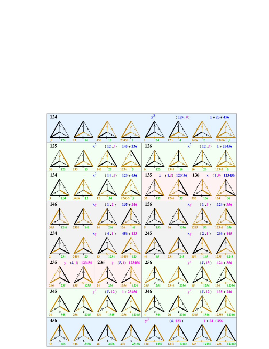
Figure 10: The canonical and refined active bijections of $K_{4}$ w.r.t. ordering and reference orientation from Figure 8

Figure 9 sums up in a table the canonical active bijection of the underlying ordered graph (Theorem 4.34). Notice that figures in previous sections are based on the same ordered graph. Figure 2 show the minors involved in the decomposition of the orientations associated with spanning tree $134$, and Figure 5 show the bijection between this orientation activity class and the interval of this spanning tree.

The reader is advised to see also [25] and [26], were more illustrations are given for constructions on the same example, such as several detailed examples of decompositions of orientations and of their active spanning trees by means of active partitions and suitably signed fundamental cycles/cocycles (represented in tableaux and in bipartite graphs), as well as a complete geometrical representation using two dual pseudoline arrangements.

Figure 10 illustrates completely the canonical and refined active bijection between orientations and spanning trees (Theorem 4.41). Each block corresponds to an activity class of orientations, and to its associated spanning tree by the canonical active bijection. The following information is given:

• In the upper left: the spanning tree $T$

• As drawn digraphs:

  • the $2^{\iota+\varepsilon}$ orientations ${\overrightarrow{G}}$ such that $T=\alpha({\overrightarrow{G}})$

  • the first orientation of the block is the active-fixed and dual-active-fixed one

• In the upper right:

  • the associated coefficient $x^{\iota}y^{\varepsilon}$ in the Tutte polynomial

  • the pair of subsets $(\mathrm{Int}(T),\mathrm{Ext}(T))=(O^{*}({\overrightarrow{G}}),O({\overrightarrow{G}}))$ whose cardinalities are $(\iota,\varepsilon)$

  • the active partition of both $T$ and ${\overrightarrow{G}}$ (reorienting the parts of the active partition provides the other graphs of a block from any of them, and, conversely, active partitions can be deduced from the set of reorientations associated with the same spanning tree by considering symmetric differences of these reorientations)

• Under each graph is illustrated the refined active bijection w.r.t. the digraph of Figure 8:

  • on the left, the corresponding reorientation with respect to the digraph of Figure 8.

  • on the right, the corresponding edge-subset obtained by adding/removing active elements with respect to the digraph of Figure 8

• On each graph:

  • the bold edges form the spanning tree

  • the grey edges are those that are reoriented

In particular, noticeable restrictions of the refined active bijection listed in Tables 1 or 3 can be read on the figure: the bijection between acyclic orientations and NBC subsets is given by the three first lines; the bijection between strongly connected orientations and supersets of external trees is given by the three last lines; the bijection between (dual-)active-fixed orientations and spanning trees is given by considering the first digraph of each block (in particular for acyclic orientations it is the only one of the block with the source of edge $1$ as unique source, yielding a bijection between such orientations and internal spanning trees); et caetera.

Acknowledgments.

Emeric Gioan wishes to thank a lot the following people: two anonymous reviewers for numerous useful comments and presentation advices, Joanna Ellis-Monaghan and Iain Moffatt for their unifying development work on the Tutte polynomial that encouraged the completion of this writing which had been pending for a long time, Bodo Lass for stimulating discussions, Clément Dupont for suggesting to use the nice term “filtration”, Ilda da Silva for useful presentation advices, and Lorenzo Traldi and Spencer Backman for some english corrections and numerous useful comments.

References

- [1] S. Backman, S. Hopkins, and L. Traldi, Fourientation activities and the Tutte polynomial, European Journal of Combinatorics 67 (2018), 40-–60
- [2] B. Benson, D. Chakrabarty, and P. Tetali, G-parking functions, acyclic orientations and spanning trees, Disc. Math. 310 (8) (2010), 1340–1353.
- [3] G. Berman, The dichromate and orientations of a graph, Canad. J. Math. 29 (1977), 947–956.
- [4] O. Bernardi, Tutte polynomial, subgraphs, orientations and sandpile model: new connections via embeddings, Electronic Journal of Combinatorics 15(1) (2008), #R109, 52p.
- [5] A. Björner, M. Las Vergnas, B. Sturmfels, N. White and G. Ziegler, Oriented matroids 2nd ed., Encyclopedia of Mathematics and its Applications 46, Cambridge University Press, Cambridge, UK 1999.
- [6] A. Blass and B.E. Sagan, Bijective proofs of two broken circuits theorems, J. Graph Theory 10 (1986), 15–21.
- [7] P. Cartier and D. Foata, Problèmes combinatoires de commutation et réarrangements, Springer-Verlag, Berlin, 1969.
- [8] H.H. Crapo, A higher invariant for matroids, J. Combinatorial Theory 2 (1967), 406–417.
- [9] H.H. Crapo, The Tutte polynomial, Aequationes Math., 3 (1969), 211–229.
- [10] J.E. Dawson, A construction for a family of sets and its application to matroids, Lect Notes in Math. (Springer) 884 (1981), 136–147, (Comb. Math. VIII, Gelong, 1980).
- [11] G. Etienne and M. Las Vergnas, External and internal elements of a matroid basis, Discrete Math. 179 (1998), 111–119.
- [12] D.D. Gebhard and B.E. Sagan, Sinks in acyclic orientations of graphs, J. Combinatorial Theory Ser. B 80 (2000), 130–146.
- [13] I. M. Gessel, Acyclic orientations and chromatic generating functions, Discrete Math., 232 (2001), 119–-130.
- [14] E. Gioan, Correspondance naturelle entre bases et réorientations des matroïdes orientés, Ph.D. thesis, University of Bordeaux 1, 2002, available at http://www.lirmm.fr/~gioan.
- [15] E. Gioan, On Tutte polynomial expansion formulas in perspectives of matroids and oriented matroids. Submitted, preprint available at arXiv:1807.06559.
- [16] E. Gioan, The Tutte polynomial of matroid perspectives, Chapter in: Handbook of the Tutte Polynomial, CRC Monographs and Research Notes in Mathematics, J. Ellis-Monaghan & I. Moffatt (Eds.), submitted.
- [17] E. Gioan, The Tutte polynomial of oriented matroids, Chapter in: Handbook of the Tutte Polynomial, CRC Monographs and Research Notes in Mathematics, J. Ellis-Monaghan & I. Moffatt (Eds.), submitted.
- [18] E. Gioan and M. Las Vergnas, Survey - On a natural correspondence between bases and reorientations, related to the Tutte polynomial and linear programming, in graphs, hyperplane arrangements, and oriented matroids, Proceedings FPSAC03 (Linköping), 26p., 2003, available at: http://www.lirmm.fr/~gioan.
- [19] E. Gioan and M. Las Vergnas, Bases, reorientations and linear programming in uniform and rank 3 oriented matroids, Adv. in Appl. Math. 32 (2004), 212–238, (Special issue Workshop on Tutte polynomials, Barcelona 2001).
- [20] E. Gioan and M. Las Vergnas, Activity preserving bijections between spanning trees and orientations in graphs, Discrete Math. 298 (2005), 169–188, (Special issue FPSAC 2002).
- [21] E. Gioan and M. Las Vergnas, The active bijection between regions and simplices in supersolvable arrangements of hyperplanes, Electronic Journal of Combinatorics 11 (2) (2006), #R30, 39p., (Stanley Festschrift).
- [22] E. Gioan and M. Las Vergnas, Fully optimal bases and the active bijection in graphs, hyperplane arrangements, and oriented matroids, Electronic Notes in Discrete Mathematics 29 (2007), 365–371, (Proceedings EuroComb 2007, Sevilla).
- [23] E. Gioan and M. Las Vergnas, A linear programming construction of fully optimal bases in graphs and hyperplane arrangements, Electronic Notes in Discrete Mathematics 34 (2009), 307–311, (Proceedings EuroComb 2009, Bordeaux).
- [24] E. Gioan and M. Las Vergnas, The active bijection in graphs, hyperplane arrangements, and oriented matroids 1. The fully optimal basis of a bounded region, European Journal of Combinatorics 30 (8) (2009), 1868–1886, (Special issue: Combinatorial Geometries and Applications: Oriented Matroids and Matroids).
- [25] E. Gioan and M. Las Vergnas, The active bijection 2.a - Decomposition of activities for matroid bases, and Tutte polynomial of a matroid in terms of beta invariants of minors. Submitted, preprint available at arXiv:1807.06516.
- [26] E. Gioan and M. Las Vergnas, The active bijection 2.b - Decomposition of activities for oriented matroids, and general definitions of the active bijection. Submitted, preprint available at arXiv:1807.06578.
- [27] E. Gioan and M. Las Vergnas, The active bijection 3. Elaborations on linear programming, in preparation.
- [28] E. Gioan and M. Las Vergnas, The active bijection 4. Deletion/contraction and universality results, in preparation.
- [29] E. Gioan and M. Las Vergnas, Computing the fully optimal spanning tree of an ordered bipolar directed graph. Submitted, preprint available at arXiv:1807.06552.
- [30] G. Gordon and E. McMahon, Interval Partitions and Activities for the Greedoid Tutte Polynomial, Adv. Appl. Math. 18 (1997), 33–49.
- [31] G. Gordon and L. Traldi, Generalized activities and the tutte polynomial, Disc. Math. 85 (1990), 167–176.
- [32] C. Greene and T. Zaslavsky, On the interpretation of whitney numbers through arrangements of hyperplanes, zonotopes, non-radon partitions and orientations of graphs, Trans. Amer. Math. Soc. 280 (1983), 97–126.
- [33] W. Kook, V. Reiner, and D. Stanton, A convolution formula for the tutte polynomial, J. Comb. Theory Ser. B 76(2) (1999), 297–300.
- [34] B. Lass, Funktionen zählen, Diplomarbeit, Universität Bonn, 148 pages, 1997.
- [35] B. Lass, Orientations acycliques et le polynôme chromatique, Europ. J. Comb 22 (2001), 1101–1123.
- [36] B. Lass, personal communication.
- [37] M. Las Vergnas, Acyclic and totally cyclic orientations of combinatorial geometries, Discrete Math. 20 (1977/78), 51-61.
- [38] M. Las Vergnas, The tutte polynomial of a morphism of matroids II. Activities of orientations, Progress in Graph Theory (J.A. Bondy & U.S.R. Murty, ed.), Academic Press, Toronto, Canada, 1984, (Proc. Waterloo Silver Jubilee Conf. 1982), pp. 367–380.
- [39] M. Las Vergnas, A correspondence between spanning trees and orientations in graphs, Graph Theory and Combinatorics (Proc. Cambridge Combin. Conf. 1983), Academic Press, London, UK 1984, 233-238.
- [40] M. Las Vergnas. The Tutte polynomial of a morphism of matroids 6. A multi-faceted counting formula for hyperplane regions and acyclic orientations. Unpublished, preliminary preprint available at arXiv 1205.5424 (2012).
- [41] M. Las Vergnas. The Tutte polynomial of a morphism of matroids 5. Derivatives as generating functions of Tutte activities. Europ. J. Comb., 34:1390–1405, 2013.
- [42] R.P. Stanley, Acyclic orientations of graphs, Discrete Math. 5 (1973), 171–178.
- [43] W.T. Tutte, A contribution to the theory of chromatic polynomials, Canad. J. Math. 6 (1954), 80–91.
- [44] W.T. Tutte, Conference given at: Workshop on Tutte polynomials, Barcelona 2001.
- [45] X.G. Viennot, Heaps of pieces, I : basic definitions and combinatorial lemmas, Lect. Notes in Math. 1234 (1986), 321–350, (Combinatoire énumérative, Proc. Colloq., Montréal Can.).
- [46] R.O. Winder, Partitions of n-space by hyperplanes, SIAM J. Applied Math. 14 (1966), 811–818.
- [47] T. Zaslavsky, Facing up to arrangements: Face-count formulas for partitions of space by hyperplanes, Mem. Amer. Math. Soc. 1 (1975), no. 154, issue 1.