Cavity Filling: Pseudo-Feature Generation for Multi-Class Imbalanced Data Problems in Deep Learning

Tomohiko Konno and Michiaki Iwazume
National Institute of Information and Communications Technology, Tokyo Japan Corresponding Author: tomohiko@nict.go.jp

(18th May 2018; \currenttime)

Abstract

Herein, we generate pseudo-features based on the multivariate probability distributions obtained from the feature maps in layers of trained deep neural networks. Further, we augment the minor-class data based on these generated pseudo-features to overcome the imbalanced data problems. The proposed method, i.e., cavity filling, improves the deep learning capabilities in several problems because all the real-world data are observed to be imbalanced.

1 Introduction: Imbalanced Data Problems

If some classes in a dataset contain few samples, the accuracy and other characteristics of these classes considerably decrease, which can cause problems during the application of machine leaning. When 90% of the data are negative and the remaining 10% are positive, an accuracy of 90% can be obtained if all the data are assumed to be negative. Therefore, positive samples are not detected. The machine learning algorithms tend to learn in a similar manner in case of imbalanced data because learning is driven by major classes containing large volumes of data. Further, a minor class contains a comparatively small volume of data.

Examples of real imbalanced data problems observed in reality include bioinfomatics [1], security [2, 3, 4, 5], finance [6], satellite imaging [7], medicine [8, 9], software development [10, 11], fault diagnosis [12], risk management [13], brain computer interface [14], medical diagnosis [15, 16], tool condition monitoring [17], activity recognition [18], video mining [19], sentiment analysis [20], behavior analysis [21], text mining [20], industrial system monitoring [22], target detection [23], software defect prediction [24], hyperspectral data analysis [25], and disease detection [26].

1.1 Existing Solutions and Background

The imbalanced data problems were reviewed in previously conducted studies [27, 28, 29]; in this subsection, typical methods for solving the imbalanced data problems will be reviewed. In the following examples, let us assume that the data contain major and minor classes with 5,000 and 500 samples each, respectively. The concept of these methods is to balance the data among various classes. Oversampling resamples minor-class data to balance them. In this example, minor classes are resampled 10 times. However, random oversampling may result in data overfitting. In contrast, undersampling reduces the major-class data for balancing the dataset. In this case, only 500 samples would be used in each major class. However, random undersampling may eliminate important data. Random elimination of the major-class data is not the only undersampling method. For instance, informed sampling, where the sampling weight is calculated, can leave important data. In this example, 4,500 of the 5,000 samples in each major class are disposed, which denotes a wastage, especially because the deep learning algorithms require large volumes of data. Thus, undersampling does not occasionally work well in deep learning. As we can observe from our experiments, undersampling improves the minor class performance; however, the total amount of data decreases, reducing the accuracy, precision, recall, and f1 scores, which may cause other problems.

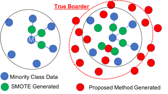
The synthetic minor class oversampling technique (SMOTE) [30] is a pseudo-data generation method. In SMOTE, the minor-class data k-neighbors are selected, and pseudo-data are generated at the interpolations of k-neighbors, as illustrated on the left side of Fig. 1. Theoretically, pseudo-data cannot cross the original determination borders in SMOTE, whereas our proposed method, i.e., cavity filling, can cross the border and push it forward, as illustrated on the right side of Fig. 1.

In deep learning feature spaces, SMOTE is used to augment data, though not for imbalanced data problems, and has been previously studied [31]. Further, we compare SMOTE in feature spaces with cavity filling and denote that our proposed method always outperforms SMOTE in the experiments.

Refer to caption — Figure 1: Left: In SMOTE, the minor-class data are randomly selected (denoted as M in the figure). Further, k-neighbors (3-neighbors in this study) are selected, and pseudo-data are generated at the interpolating points. Right: Even though the pseudo-data generated by SMOTE cannot go beyond the determination border, our proposed method can go beyond the border and push it forward near to the true determination border.

The weight-adjusted loss function exists in addition to the sampling methods. A weight-adjusted loss function aims to reduce the weights of the major classes and increase those of the minor classes in the loss function. In our example, the minor-class losses increase by $10$ times when compared with the major-class losses.

Bagging and boosting: Many methods are available to reduce the major-class data from 5,000 to 500 in undersampling. Further, the corresponding classifiers can be constructed, and ensemble learning can be achieved using these classifiers. Ensemble learning with undersampling is a good methodology [32]; however, ensemble learning can be computationally expensive in case of deep learning.

Combination of methods: In real applications, we solve imbalanced data using various combinations of methods and do not use only a single method. Therefore, we add one method that is worth testing to other methods.

1.1.1 Background: Recent Progress and Success in Deep Learning

As will be clarified by the remainder of this study, the success of our proposed method can be attributed to the achievements in deep learning. Deep neural networks accurately capture the feature distributions; thus, multidimensional probability distributions that accurately fit the features can be obtained. It was not until recent progress and success in deep learning that our proposed method would have been possible. Thus, our proposed method belongs to the deep learning age.

1.2 Contributions

The contributions of our study can be given as follows.

1.

We propose a method named “cavity filling” to synthesize pseudo-features based on the multivariate probability distributions obtained from feature maps in a layer of trained deep neural networks.
2.

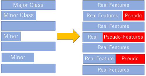
We virtually increase the data volume in minor classes using the generated pseudo-feature and make progress in multi-class imbalanced data problems in deep learning.

In cavity filling, we use the existing networks, such as ResNet [33], in the experiments, and we do not have to modify the successful network structures, which is an advantage of our proposed method. Changing the structures of the existing successful networks may cause decreased performance.

1.3 Recent Works

Recent works on imbalanced data can be summarized as follows. The methods for imbalanced data in convolutional neural networks were compared[34], and instance selections and geometric mean accuracy were studied [35]. Further, the cost-sensitive deep belief networks were studied [36], and a cost function approach, i.e., class rectification loss, was studied [37]. The neighbors progressive competitive algorithm, inspired by the k-nearest neighbor, has also been proposed [38]. A boosting method known as locality informed under-boosting was proposed in a previous study [39]. Furthermore, an imbalanced cardiovascular medical dataset was previously studied [40].Supplemental data selection for data rebalancing was also studied [41]. An approach to train the generative adversarial networks using imbalanced data and to generate the minor-class images was studied in [42], and an example reweighing algorithm for deep learning was investigated [43]. A sampling method with a loss function, i.e., quintuplet sampling with triple-header loss, was also previously investigated [44].

2 The Proposed Method: Cavity Filling

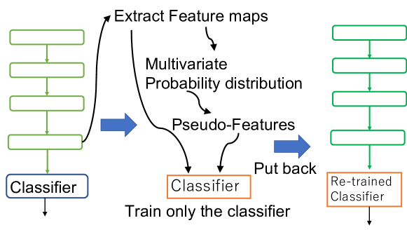
Our proposed method can be explained as follows. We require two-stage training. Fig. 2 and Fig. 3 depict the diagrams of the procedure and its main idea, respectively.

Step 1:

Train deep neural networks.
Step 2:

Extract feature maps from a layer.
Step 3:

Obtain multivariate probability distributions of these feature maps.
Step 4:

Generate pseudo-features from the multivariate probability distributions to obtain pseudo-features of the minor classes.
Step 5:

Train the layers following the layer from which features were extracted based on the real features and pseudo-features. Only the classifier layers are updated.
Step 6:

Return the trained classifier layers to the original network and use the newly combined network for performing the estimation.

In the experiments, deep neural networks are trained using the original imbalanced data. Further, features are extracted from the layer immediately before the classifier layer and a multivariate Gaussian method is used to parameterize the features. We observed that the multivariate Gaussian method works better than an independent Gaussian method comprising independent random variables assigned to each feature-map dimension in the experiments. The final classifier is retrained based on the real features and pseudo-features, and the retrained classifier is returned to the network.

3 Experiments on Multi-Class Imbalanced Data Problem

We synthesized an imbalanced dataset using Cifar10 [45] and Imagenet [46] datasets. Subsequently, we conducted two experiments using the imbalanced dataset.

We assume that we need some amount of data, even for minor classes, because cavity filling considerably relies on the deep-learning captured features. However, in the deep learning age, private companies possess large datasets with large volumes of data, even for minor classes. In this situation, cavity filling works appropriately.

3.1 Synthesizing the Multi-Class Imbalanced Data (Cifar10)

We synthesized imbalanced data from cifar10 [45] because it is a standard benchmark dataset. In cifar10, $10$ classes are present with $5,000$ samples in each class. Thus, the total number of samples in the training data and test data is $50,000$ and $10,000$ , respectively. Subsequently, we determine the number of classes that can be considered minor classes and randomly select these classes; the remaining classes become major classes. We then reduce the data volume in minor classes by a factor of $10$ . Thus, minor classes contain $500$ samples, whereas major classes contain $5,000$ samples in our experiments¹¹1if we consider minor classes in a similar manner using cifar100, each minor class would contain only $50$ samples, which is not suited for deep learning..

3.2 Comparison of Methods (Cifar10)

The baseline denotes training using the original imbalanced data. In the experiments, undersampling indicates that the major-class data are randomly reduced from $5,000$ to $500$ to balance the classes. Thus, oversampling denotes that the $500$ minor-class data are resampled $5,000$ times. SMOTE²²2The python package ”imbalanced-learn” [47] is used. contains training of the classifier based on the real features and added pseudo-features made by SMOTE in the feature space. Perturbed denotes training of the classifier with additional perturbed features of multidimensional Gaussian noise, which has a mean of $0$ and a variance calculated based on the real features of the training data. Finally, proposed denotes the proposed method, i.e., cavity filling. Pseudo-features are generated in SMOTE, perturbed, and proposed; thus, the real and pseudo-features constitute balanced data. More specifically, $4500$ pseudo-features are produced for each minor class.

3.3 Experimental Flow (Cifar10)

We changed the number of minor classes from $1$ to $9$ and performed experiments as follows.

1.

Select the number of minor classes, varying from $1$ to $9$ throughout the experiment.
2.

Use $500$ from among $5,000$ samples in minor classes, producing imbalanced data from cifar10. The imbalance ratio is $1$ to $10$ .
3.

By keeping the minor classes fixed, the baseline, undersampling, oversampling, SMOTE, perturbed, and cavity filling methods are compared.

Keras [48] and ResNet56 [33] are used, with a batch size of $128$ , an optimizer of Adam, and epochs of $100$ . The test data are original cifar10 test data.

3.4 Experimental Results (Cifar10)

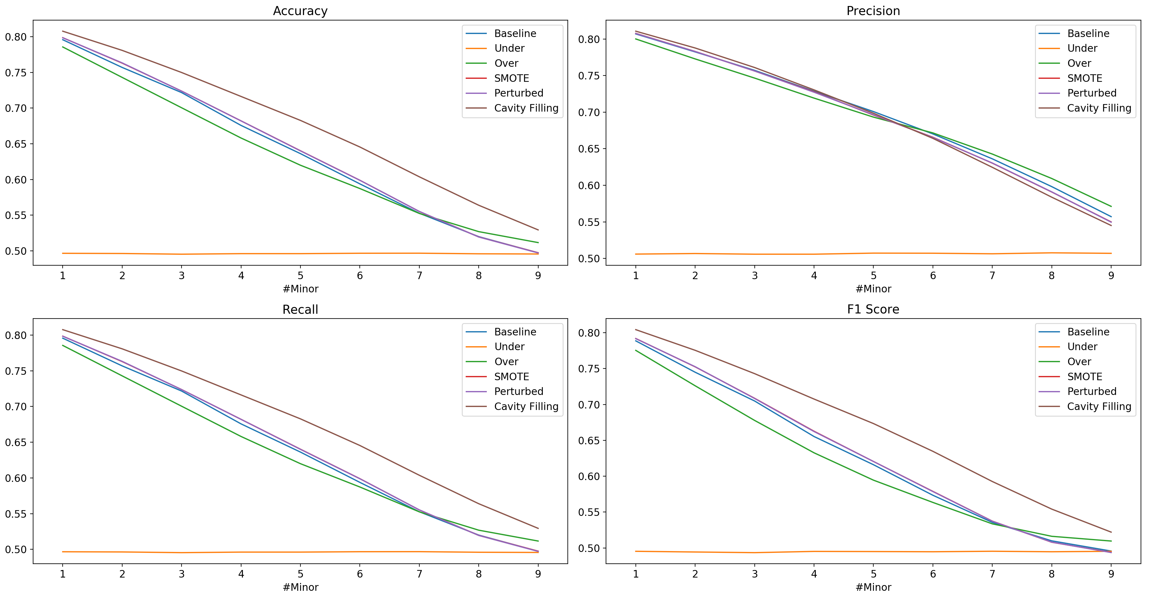
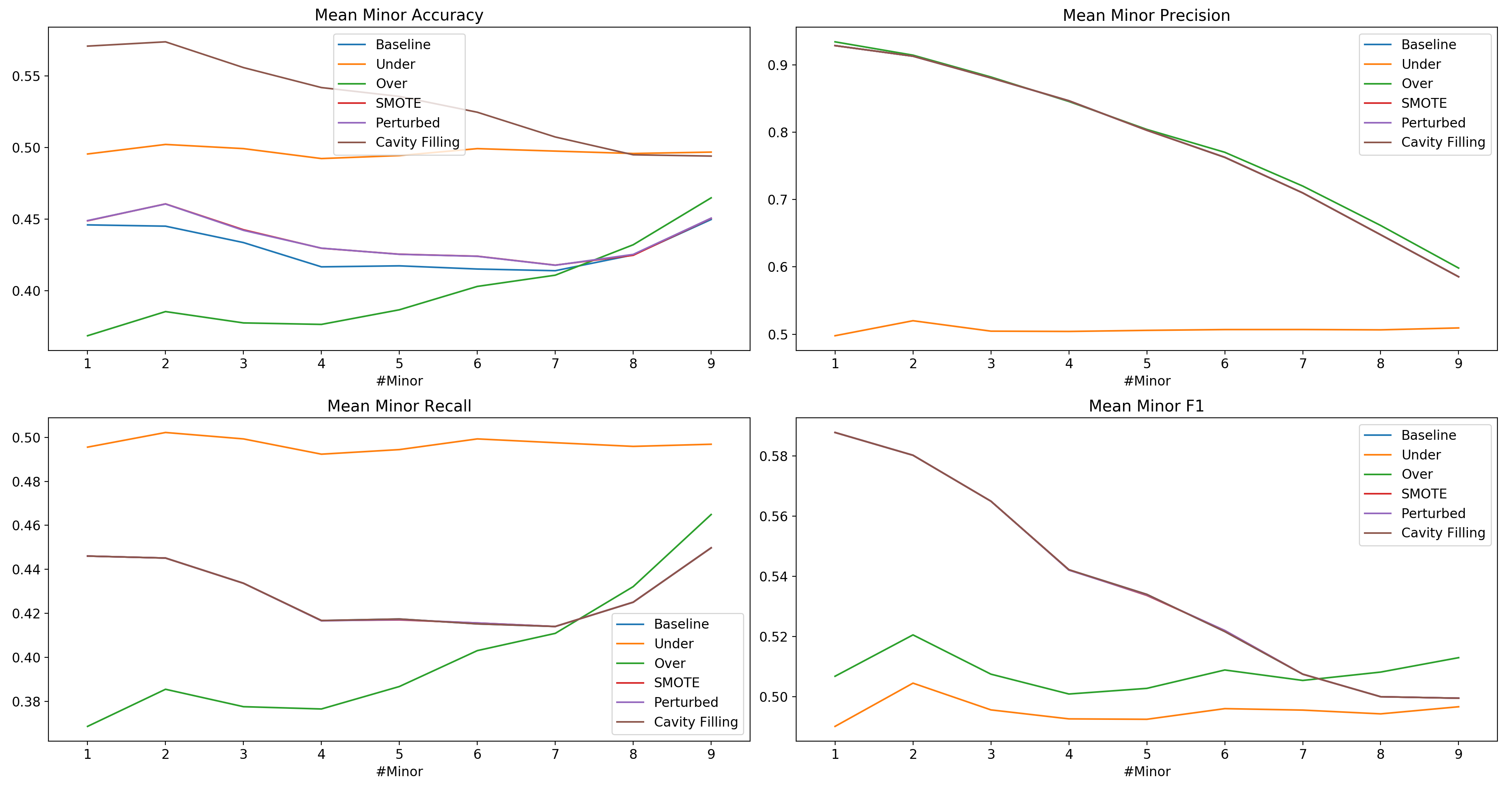
The experimental results are the averages obtained over 144 episodes. One episode indicates a sequence of experiments in which the number of minor classes changes from $1$ to $9$ . #Minor denotes the number of minor classes and does not represent a class identification number. If #Minor is $4$ , $4$ out of $10$ classes contain only $500$ samples, whereas the remaining classes contain $5,000$ samples. Once the minor classes were determined, we performed baseline, undersampling, oversampling, SMOTE, perturbed, and cavity filling methods while keeping the minor classes fixed.

The results are illustrated in Fig. 5 and Fig. 5. In Fig. 5, the accuracy is for the whole data, whereas the precision, recall, and F1 are macro averages for each class. The proposed method is much better in terms of accuracy, recall, and F1 and is as good as other methods with respect to the precision.

We also verified the mean accuracy, precision, recall, and F1 of the minor classes alone ,and they are the macro averages over minor classes because the scores in minor classes are important at times. They are illustrated in Fig. 5. Undersampling, SMOTE, perturbation, and cavity filling exhibit identical mean precision, recall, and F1 scores of minor classes and cannot be distinguished in the figures. The scores are summarized in Tab. 5–Tab. 5 in the appendix. Although undersampling exhibits improved mean minor recall, cavity filling is better than or as good as undersampling and oversampling with respect to the mean minor accuracy, precision, and F1. Further, cavity filling and undersampling can be combined. We can use undersampling and cavity filling for other cases when the recall of minor classes is important.

3.5 Experiment on Multi-Class Imbalanced Data Obtained from ImageNet

We synthesized imbalanced data from ImageNet, comprising $1,000$ image classes and approximately $13$ M images. Further, we produced imbalanced data from ImageNet as follows. First, we chose $500$ minor classes among $1,000$ classes. Then, we reduced the number of images in minor classes by a factor of $10$ , yielding an imbalance ratio of $10$ to $1$ .

Table 1: Scores for imbalanced data produced from ImageNet

	Accuracy	Precision	Recall	F1
baseline	49.9	51.5	43.6	40.0
undersampling	29.7	29.0	29.5	29.0
over sampling	49.5	51.6	43.9	40.7
SMOTE	53.5	55.2	53.4	52.8
Cavity Filling	54.2	55.0	54.1	53.5

We used the Resnet34 neural network, an optimizer of Adam, no data augmentation, a batch size of $256$ , and an epoch of $100$ . The baseline values in the table are for the as-is imbalanced data and accuracy for the original test data. The precision, recall, F1 are macro averages over each class; therefore, they are low. However, they are improved by cavity filling. The results are summarized in Table 1. Cavity filling improves the accuracy by $4.3\%$ from baseline, making it better than SMOTE.

4 Conclusion

We propose a method named cavity filling, which generates pseudo-features to fill the gaps between the minor and major classes in feature spaces. Further, we extract features from a layer of trained deep neural network, obtain multivariate probability distributions from the features of each minor class, and sample the minor-class pseudo-features from multivariate probability to virtually increase the minor-class training data. We do not generate pseudo-data but generate pseudo-features. Subsequently, we train the layers following the layer from which features were extracted based on the pseudo-features and real features. The cavity filling method functions in an appropriate manner for multi-class imbalanced data.

References

[1] Nicolás García-Pedrajas, Javier Pérez-Rodríguez, María García-Pedrajas, Domingo Ortiz-Boyer, and Colin Fyfe. Class imbalance methods for translation initiation site recognition in dna sequences. Knowledge-Based Systems, 25(1):22–34, 2012.
[2] David A Cieslak, Nitesh V Chawla, and Aaron Striegel. Combating imbalance in network intrusion datasets. In GrC, pages 732–737, 2006.
[3] Andrea Dal Pozzolo, Olivier Caelen, Yann-Ael Le Borgne, Serge Waterschoot, and Gianluca Bontempi. Learned lessons in credit card fraud detection from a practitioner perspective. Expert systems with applications, 41(10):4915–4928, 2014.
[4] Abebe Tesfahun and D Lalitha Bhaskari. Intrusion detection using random forests classifier with smote and feature reduction. In Cloud & Ubiquitous Computing & Emerging Technologies (CUBE), 2013 International Conference on, pages 127–132. IEEE, 2013.
[5] Clifton Phua, Damminda Alahakoon, and Vincent Lee. Minority report in fraud detection: classification of skewed data. Acm sigkdd explorations newsletter, 6(1):50–59, 2004.
[6] José Antonio Sanz, Dario Bernardo, Francisco Herrera, Humberto Bustince, and Hani Hagras. A compact evolutionary interval-valued fuzzy rule-based classification system for the modeling and prediction of real-world financial applications with imbalanced data. IEEE Transactions on Fuzzy Systems, 23(4):973–990, 2015.
[7] Baojuan Zheng, Soe W Myint, Prasad S Thenkabail, and Rimjhim M Aggarwal. A support vector machine to identify irrigated crop types using time-series landsat ndvi data. International Journal of Applied Earth Observation and Geoinformation, 34:103–112, 2015.
[8] Simon F Eskildsen, Pierrick Coupé, Vladimir Fonov, and D Louis Collins. Detecting alzheimer’s disease by morphological mri using hippocampal grading and cortical thickness. In Proc MICCAI workshop Challenge on Computer-Aided Diagnosis of Dementia Based on Structural MRI Data, pages 38–47, 2014.
[9] Bartosz Krawczyk, Mikel Galar, Łukasz Jeleń, and Francisco Herrera. Evolutionary undersampling boosting for imbalanced classification of breast cancer malignancy. Applied Soft Computing, 38:714–726, 2016.
[10] Salvador García and Francisco Herrera. Evolutionary undersampling for classification with imbalanced datasets: Proposals and taxonomy. Evolutionary computation, 17(3):275–306, 2009.
[11] RA Mollineda, R Alejo, and JM Sotoca. The class imbalance problem in pattern classification and learning. In II Congreso Español de Informática (CEDI 2007). ISBN, pages 978–84, 2007.
[12] Chong Zhang, Jia Hui Sun, and Kay Chen Tan. Deep belief networks ensemble with multi-objective optimization for failure diagnosis. In Systems, Man, and Cybernetics (SMC), 2015 IEEE International Conference on, pages 32–37. IEEE, 2015.
[13] Kazuo J Ezawa, Moninder Singh, and Steven W Norton. Learning goal oriented bayesian networks for telecommunications risk management. In ICML, pages 139–147, 1996.
[14] Sim Kuan Goh, Hussein A Abbass, Kay Chen Tan, and Abdullah Al Mamun. Artifact removal from eeg using a multi-objective independent component analysis model. In International Conference on Neural Information Processing, pages 570–577. Springer, 2014.
[15] Rosa Maria Valdovinos and José Salvador Sánchez. Class-dependant resampling for medical applications. In Machine Learning and Applications, 2005. Proceedings. Fourth International Conference on, pages 6–pp. IEEE, 2005.
[16] Jerzy W Grzymala-Busse, Linda K Goodwin, Witold J Grzymala-Busse, and Xinqun Zheng. An approach to imbalanced data sets based on changing rule strength. In Rough-Neural Computing, pages 543–553. Springer, 2004.
[17] J Sun, M Rahman, YS Wong, and GS Hong. Multiclassification of tool wear with support vector machine by manufacturing loss consideration. International Journal of Machine Tools and Manufacture, 44(11):1179–1187, 2004.
[18] Xingyu Gao, Zhenyu Chen, Sheng Tang, Yongdong Zhang, and Jintao Li. Adaptive weighted imbalance learning with application to abnormal activity recognition. Neurocomputing, 173:1927–1935, 2016.
[19] Zan Gao, Long-fei Zhang, Ming-yu Chen, Alexander Hauptmann, Hua Zhang, and An-Ni Cai. Enhanced and hierarchical structure algorithm for data imbalance problem in semantic extraction under massive video dataset. Multimedia tools and applications, 68(3):641–657, 2014.
[20] Tsendsuren Munkhdalai, Oyun-Erdene Namsrai, and Keun Ho Ryu. Self-training in significance space of support vectors for imbalanced biomedical event data. BMC bioinformatics, 16(7):S6, 2015.
[21] Amos Azaria, Ariella Richardson, Sarit Kraus, and VS Subrahmanian. Behavioral analysis of insider threat: A survey and bootstrapped prediction in imbalanced data. IEEE Transactions on Computational Social Systems, 1(2):135–155, 2014.
[22] Enislay Ramentol, I Gondres, S Lajes, Rafael Bello, Yaile Caballero, Chris Cornelis, and Francisco Herrera. Fuzzy-rough imbalanced learning for the diagnosis of high voltage circuit breaker maintenance: The smote-frst-2t algorithm. Engineering Applications of Artificial Intelligence, 48:134–139, 2016.
[23] Sébastien Razakarivony and Frédéric Jurie. Vehicle detection in aerial imagery: A small target detection benchmark. Journal of Visual Communication and Image Representation, 34:187–203, 2016.
[24] José A Sáez, Julián Luengo, Jerzy Stefanowski, and Francisco Herrera. Smote–ipf: Addressing the noisy and borderline examples problem in imbalanced classification by a re-sampling method with filtering. Information Sciences, 291:184–203, 2015.
[25] Yanmin Sun, Andrew KC Wong, and Mohamed S Kamel. Classification of imbalanced data: A review. International Journal of Pattern Recognition and Artificial Intelligence, 23(04):687–719, 2009.
[26] K. C. L. Wong, A. Karargyris, T. Syeda-Mahmood, and M. Moradi. Building Disease Detection Algorithms with Very Small Numbers of Positive Samples. ArXiv e-prints, May 2018.
[27] Haibo He and Edwardo A Garcia. Learning from imbalanced data. IEEE Transactions on knowledge and data engineering, 21(9):1263–1284, 2009.
[28] Mikel Galar, Alberto Fernandez, Edurne Barrenechea, Humberto Bustince, and Francisco Herrera. A review on ensembles for the class imbalance problem: bagging-, boosting-, and hybrid-based approaches. IEEE Transactions on Systems, Man, and Cybernetics, Part C (Applications and Reviews), 42(4):463–484, 2012.
[29] Bartosz Krawczyk. Learning from imbalanced data: open challenges and future directions. Progress in Artificial Intelligence, 5(4):221–232, Nov 2016.
[30] Nitesh V Chawla, Kevin W Bowyer, Lawrence O Hall, and W Philip Kegelmeyer. Smote: synthetic minority over-sampling technique. Journal of artificial intelligence research, 16:321–357, 2002.
[31] T. DeVries and G. W. Taylor. Dataset Augmentation in Feature Space. ArXiv e-prints, February 2017.
[32] Byron C Wallace, Kevin Small, Carla E Brodley, and Thomas A Trikalinos. Class imbalance, redux. In Data Mining (ICDM), 2011 IEEE 11th International Conference on, pages 754–763. IEEE, 2011.
[33] Kaiming He, Xiangyu Zhang, Shaoqing Ren, and Jian Sun. Deep residual learning for image recognition. arXiv preprint arXiv:1512.03385, 2015.
[34] M. Buda, A. Maki, and M. A. Mazurowski. A systematic study of the class imbalance problem in convolutional neural networks. ArXiv e-prints, October 2017.
[35] L. I. Kuncheva, Á. Arnaiz-González, J.-F. Díez-Pastor, and I. A. D. Gunn. Instance Selection Improves Geometric Mean Accuracy: A Study on Imbalanced Data Classification. ArXiv e-prints, April 2018.
[36] C. Zhang, K. C. Tan, H. Li, and G. S. Hong. A Cost-Sensitive Deep Belief Network for Imbalanced Classification. ArXiv e-prints, April 2018.
[37] Q. Dong, S. Gong, and X. Zhu. Class Rectification Hard Mining for Imbalanced Deep Learning. ArXiv e-prints, December 2017.
[38] S. Saryazdi, B. Nikpour, and H. Nezamabadi-pour. NPC: Neighbors Progressive Competition Algorithm for Classification of Imbalanced Data Sets. ArXiv e-prints, November 2017.
[39] S. Ahmed, F. Rayhan, A. Mahbub, M. Rafsan Jani, S. Shatabda, D. M. Farid, and C. Mofizur Rahman. LIUBoost : Locality Informed Underboosting for Imbalanced Data Classification. ArXiv e-prints, November 2017.
[40] Md. Mostafizur Rahman and Darryl N. Davis. Addressing the class imbalance problem in medical datasets. 2013.
[41] J. McKay, I. Gerg, and V. Monga. Bridging the Gap: Simultaneous Fine Tuning for Data Re-Balancing. ArXiv e-prints, January 2018.
[42] G. Mariani, F. Scheidegger, R. Istrate, C. Bekas, and C. Malossi. BAGAN: Data Augmentation with Balancing GAN. ArXiv e-prints, March 2018.
[43] M. Ren, W. Zeng, B. Yang, and R. Urtasun. Learning to Reweight Examples for Robust Deep Learning. ArXiv e-prints, March 2018.
[44] Chen Huang, Yining Li, Chen Change Loy, and Xiaoou Tang. Learning deep representation for imbalanced classification. In Proceedings of the IEEE Conference on Computer Vision and Pattern Recognition, pages 5375–5384, 2016.
[45] Alex Krizhevsky and Geoffrey Hinton. Learning multiple layers of features from tiny images. 2009.
[46] Olga Russakovsky, Jia Deng, Hao Su, Jonathan Krause, Sanjeev Satheesh, Sean Ma, Zhiheng Huang, Andrej Karpathy, Aditya Khosla, Michael Bernstein, Alexander C. Berg, and Li Fei-Fei. ImageNet Large Scale Visual Recognition Challenge. International Journal of Computer Vision (IJCV), 115(3):211–252, 2015.
[47] Guillaume Lemaître, Fernando Nogueira, and Christos K. Aridas. Imbalanced-learn: A python toolbox to tackle the curse of imbalanced datasets in machine learning. Journal of Machine Learning Research, 18(17):1–5, 2017.
[48] Francois Chollet et al. Keras. https://github.com/fchollet/keras, 2015.

Competing Interests: The authors declare that they have no competing financial interests.
Correspondence: Correspondence and requests for materials should be addressed to Tomohiko Konno (tomohiko@nict.go.jp).

Appendix A Mean scores of the minor classes (Cifar10)

The tables that summarize the macro averaged scores for minor classes in Cifar10 are presented here because some points are difficult to distinguish in the figures. Under represents undersampling, Over represents oversampling, and Perturbed represents perturbation.

#Minor	Baseline	Under	Over	SMOTE	Perturbed	Cavity Filling
1	0.45	0.50	0.37	0.45	0.45	0.57
2	0.45	0.50	0.39	0.46	0.46	0.57
3	0.43	0.50	0.38	0.44	0.44	0.56
4	0.42	0.49	0.38	0.43	0.43	0.54
5	0.42	0.49	0.39	0.43	0.43	0.54
6	0.42	0.50	0.40	0.42	0.42	0.52
7	0.41	0.50	0.41	0.42	0.42	0.51
8	0.43	0.50	0.43	0.42	0.43	0.50
9	0.45	0.50	0.46	0.45	0.45	0.49

Table 2: Mean Minor Accuracy

#Minor	Baseline	Under	Over	SMOTE	Perturbed	Cavity Filling
1	0.93	0.50	0.93	0.93	0.93	0.93
2	0.91	0.52	0.91	0.91	0.91	0.91
3	0.88	0.50	0.88	0.88	0.88	0.88
4	0.85	0.50	0.85	0.85	0.85	0.85
5	0.80	0.51	0.80	0.80	0.80	0.80
6	0.76	0.51	0.77	0.76	0.76	0.76
7	0.71	0.51	0.72	0.71	0.71	0.71
8	0.65	0.51	0.66	0.65	0.65	0.65
9	0.59	0.51	0.60	0.59	0.59	0.59

Table 3: Mean Minor Precision

#Minor	Baseline	Under	Over	SMOTE	Perturbed	Cavity Filling
1	0.45	0.50	0.37	0.45	0.45	0.45
2	0.45	0.50	0.39	0.45	0.45	0.45
3	0.43	0.50	0.38	0.43	0.43	0.43
4	0.42	0.49	0.38	0.42	0.42	0.42
5	0.42	0.49	0.39	0.42	0.42	0.42
6	0.42	0.50	0.40	0.42	0.42	0.42
7	0.41	0.50	0.41	0.41	0.41	0.41
8	0.43	0.50	0.43	0.43	0.43	0.43
9	0.45	0.50	0.46	0.45	0.45	0.45

Table 4: Mean Minor Recall

#Minor	Baseline	Under	Over	SMOTE	Perturbed	Cavity Filling
1	0.59	0.49	0.51	0.59	0.59	0.59
2	0.58	0.50	0.52	0.58	0.58	0.58
3	0.56	0.50	0.51	0.56	0.56	0.56
4	0.54	0.49	0.50	0.54	0.54	0.54
5	0.53	0.49	0.50	0.53	0.53	0.53
6	0.52	0.50	0.51	0.52	0.52	0.52
7	0.51	0.50	0.51	0.51	0.51	0.51
8	0.50	0.49	0.51	0.50	0.50	0.50
9	0.50	0.50	0.51	0.50	0.50	0.50

Table 5: Mean Minor F1