Effects of the Dirac cone tilt in two-dimensional Dirac semimetal

Abstract

Two-dimensional Dirac semimetal with tilted Dirac cone has recently attracted increasing interest. Tilt of Dirac cone can be realized in a number of materials, including deformed graphene, surface state of topological crystalline insulator, and certain organic compound. We study how Dirac cone tilting affects the low-energy properties by presenting a renormalization group analysis of the Coulomb interaction and quenched disorder. Random scalar potential or random vector potential along the tilting direction cannot exist on its own as it always dynamically generates a new type of disorder, which dominates at low energies and turns the system into a compressible diffusive metal. Consequently, the fermions acquire a finite disorder scattering rate. Moreover, the isolated band-touching point is replaced by a bulk Fermi arc in the Brillouin zone. These results are not qualitatively changed when the Coulomb interaction is incorporated. In comparison, random mass and random vector potential along the non-tilting direction can exist individually, without generating other types of disorder. They both suppress tilt at low energies, and do not produce bulk Fermi arc. Upon taking the Coulomb interaction into account, the system enters into a stable quantum critical state, in which the fermion field acquires a finite anomalous dimension but the dynamical exponent $z=1$. These results indicate that Dirac cone tilt does lead to some qualitatively different low-energy properties comparing to the untilted system.

I Introduction

Semimetal (SM) materials have been studied for more than one decade CastroNeto09 ; Kotov12 ; Vafek14 ; Wehling14 ; Wan11 ; Weng16 ; FangChen16 ; Yan17 ; Hasan17 ; Armitage18 . They exhibit many unusual properties different from ordinary metals and semiconductors. Among all the currently known SMs, two-dimensional (2D) Dirac SM (DSM) has attracted particular interest. Graphene CastroNeto09 ; Kotov12 and the surface state of three-dimensional (3D) topological insulator Vafek14 ; Wehling14 are two sorts of 2D DSM. A prominent feature of 2D DSM is that, the fermion density of states (DOS) vanishes at the Fermi level. Thus the Coulomb interaction is long-ranged and may induce nontrivial quantum corrections to various observable quantities Kotov12 . This is quite different from ordinary metals in which the Coulomb interaction is statically screened by the finite zero-energy DOS and can be safely neglected GiulianiBook ; ColemanBook ; Shankar94 .

In an intrinsic graphene, the conduction band exhibits an almost perfect cone shape near the Dirac point. In many realistic DSM materials, however, the Dirac cone is more or less distorted. It is known that tilted Dirac cone can be realized in a number of materials, including properly deformed graphene Goerbig08 ; Choi10 , organic compound $\alpha$-(BEDT-TTF)₂I₃ Goerbig08 ; Kobayashi07 ; Hirata16 ; Hirata17 , 8-$Pmmn$ borophene Zhou14 ; Zobolotskiy16 ; Feng17 ; Sadhukhan17 ; Verma17 ; Islam17 , and partially hydrogenated graphene Lu16 . In addition, the surface of topological crystalline insulators, such as the (001) surface of SnSe Tanaka12 ; Sodemann15 , may also host a tilted Dirac cone. Recent study Varyhalov17 suggests that a tilted Dirac cone appears on the (110) surface of W, which is not caused by topology but arises from Rashba split bands. To understand the properties of these materials, it is necessary to study the physical effects induced by the tilt of Dirac cone. In particular, we wish to examine whether the tilt leads to qualitatively new physics. This is the primary motivation of the present work.

For simplicity, we suppose that the Dirac cone is only moderately tilted such that the Fermi surface is still made out of discrete zero-dimensional points. In the clean limit, the fermion DOS vanishes at Fermi level. Isobe and Nagaosa Isobe12 have analyzed the impact of long-range Coulomb interaction and revealed that it is marginally irrelevant. The tilt parameter flows gradually to zero in the lowest energy limit Isobe12 . This conclusion is confirmed by a more recent work LeeLee18 . It turns out that tilted DSM exhibits very similar properties to untilted DSM in the clean limit. However, coupling to disorders may drastically change the low-energy behaviors of fermions Papaj18 ; Zhao18 .

In this paper, we present a renormalization group (RG) study of the impact of several types of ordinary disorder that commonly exist in realistic DSM samples, including random scalar potential (RSP), random vector potential (RVP), and random mass (RM). We are also interested in the physical effects of the combination of Coulomb interaction and disorder. It will become clear that the tilt does lead to interesting properties that are not realized in the untilted system.

In a untilted 2D DSM, every type of quenched disorder, including RSP, two components of RVP, and RM, can exist on its own without generating other types of disorder Ludwig94 ; Ostrovsky06 ; Evers08 ; Foster12 . The two components of RVP, abbreviated as $x$-RVP and $y$-RVP, are equivalent. These features are significantly changed by the Dirac cone tilt. Without loss of generality, we suppose the tilt is along $x$-axis. We will show that, RSP cannot exist alone in the system: it always dynamically generates a new type of disorder that is originally absent. Remarkably, the generated disorder is dominant at low energies and its strength parameter flows to the strong coupling regime. As a consequence, the system is turned into compressible diffusive metal (CDM) phase, in which the fermions acquire a finite disorder scattering rate. Moreover, the original Dirac point is replaced by a bulk Fermi arc. The $x$-RVP leads to almost the same physical consequences as RSP. However, $y$-RVP plays an entirely different role from $x$-RVP, and also from RSP. Interestingly, $y$-RVP can exist alone in tilted 2D DSM, and it completely suppresses the tilt. In the low-energy region, $y$-RVP is marginal, leading to power-law corrections to the energy or temperature dependence of observable quantities. Analogous to $y$-RVP, RM can also exist independently, and it also tends to suppress tilt. But RM is marginally irrelevant in the low-energy region and thus only induces logarithmic-like corrections to observable quantities.

We see that dirty tilted 2D DSM exhibits distinct physics comparing to the clean system. It is interesting to investigate how these results are affected by the Coulomb interaction. In the cases of RSP and $x$-RVP, the Coulomb interaction is much less important, and the system is still turned into CDM that exhibits bulk Fermi arc. If there is no tilt, strong Coulomb interaction dominates RSP at low energies and protects the SM phase, whereas the interplay of Coulomb interaction and $x$-RVP leads to a stable quantum critical state featuring vanishing DOS at Fermi level. Obviously, this difference is caused by the tilt. When the Coulomb interaction cooperates with $y$-RVP or RM, the tilt flows to zero in the lowest energy limit, and the system enters into a stable quantum critical state, where the fermion field acquires a finite anomalous dimension but the dynamical exponent is $z=1$. To gain a better understanding of this critical state, we calculate several observable quantities, such as fermion DOS, specific heat, and compressibility, and analyze their energy or temperature dependence.

The rest of the paper will be organized as follows. The effective model for tilted 2D Dirac fermions is described in Sec. II. The dynamical generation of new type of disorder is discussed in this section. The coupled RG equations for various model parameters are presented in Sec. III. The numerical results for the RG equations and their physical implications are analyzed in Sec. IV. In Sec. V, the main results obtained in this work are summarized and compared to previous works. Detailed RG calculations are presented in Appendix A. Observable quantities are calculated in Appendixes B and C. In Appendix D, we present the RG results obtained by omitting the dynamically generated fermion-disorder coupling.

II Effective Model

We suppose that the Dirac cone is tilted along $x$-axis. The free Hamiltonian for 2D tilted Dirac fermions is

$$H=\int_{\mathbf{x}}\psi^{{\dagger}}(\mathbf{x})\left[-v_{x}\left(t\sigma_{0}+\sigma_{x}\right)i\partial_{x}-v_{y}\sigma_{y}i\partial_{y}\right]\psi(\mathbf{x}),$$ (1)

where $\int_{\mathbf{x}}\equiv\int d^{2}\mathbf{x}$ and $\psi$ is a two-component spinor. There are $N$ copies of $\psi$, where $N$ can be identified as the fermion flavor. For graphene, the two components of $\psi$ correspond to the two sublattices $A$ and $B$. The physical fermion flavor Kotov12 ; Vafek07 ; Sheehy07 is $N=4$, which originates from the two valleys ($K$, $K^{\prime}$) and the two spins ($\uparrow$, $\downarrow$). $\sigma_{x}$ and $\sigma_{y}$ are two Pauli matrices, and $\sigma_{0}$ is identity matrix. The energy dispersion of fermions is defined as

$$E_{\pm}=tv_{x}k_{x}\pm\sqrt{v_{x}^{2}k_{x}^{2}+v_{y}^{2}k_{y}^{2}},$$ (2)

where $v_{x}$ and $v_{x}$ are two velocities. The tilt parameter is $t$ with $t=0$ corresponding to untilted Dirac cone. For $|t|<1$, the system is identified as type-I DSM, in which the Fermi surface is made out of discrete band-touching points. For $|t|>1$, the system corresponds to type-II DSM, whose Fermi surface is a finite open line LeeLee18 ; Soluyanov15 ; Isobe16TyepII ; Huang17 . The fermion DOS vanishes at the Fermi level in type-I DSM, but takes a finite value in type-II DSM. Physically, $t<0$ or $t>0$ are equivalent, thus we only consider the case of $0<t<1$ hereafter.

The Hamiltonian for Coulomb interaction is

$$H_{C}=\frac{1}{4\pi}\int d^{2}\mathbf{x}d^{2}\mathbf{x}^{\prime}\rho(\mathbf{x})\frac{e^{2}}{\epsilon\left|\mathbf{x}-\mathbf{x}^{\prime}\right|}\rho(\mathbf{x}^{\prime}),$$ (3)

where $\rho(\mathbf{x})=\psi^{{\dagger}}(\mathbf{x})\psi(\mathbf{x})$ is fermion density, $e$ electric charge and $\epsilon$ dielectric constant. The role of Coulomb interaction depends on the fermion dispersion and dimension Gonzalez99 ; Son07 ; Barnes14 ; Hofmann14 ; Sharma16 ; Goswami11 ; Hosur12 ; Gonzalez14 ; Hofmann15 ; Throckmorton15 ; Sharma18 ; Yang14 ; Abrikosov72 ; Abrikosov71 ; Abrikosov74 ; Moon13 ; Herbut14 ; Janssen15 ; Dumitrescu15 ; Janssen16 ; Janssen17 ; Huh16 ; Isobe16A ; Cho16 ; Isobe16B ; Lai15 ; Jian15 ; Zhang17 ; Isobe12 ; Detassis17 ; LeeLee18 . RG studies found that Coulomb interaction is marginally irrelevant in 2D DSM and induces logarithmic-like corrections to the energy, momenta, or temperature dependence of observable quantities Kotov12 ; Gonzalez99 ; Son07 ; Barnes14 ; Hofmann14 . For instance, the fermion velocity is predicted to acquire a logarithmic-like momenta-dependence Kotov12 ; Gonzalez99 ; Son07 ; Barnes14 ; Hofmann14 , consistent with experiments Elias11 ; Siegel11 ; Yu13 ; Miao13 ; Faugeras15 .

The free fermion propagator is

$$G_{0}\left(i\omega,\mathbf{k}\right)=\frac{1}{i\omega\sigma_{0}-\left(t\sigma_{0}+\sigma_{x}\right)v_{x}k_{x}-v_{y}k_{y}\sigma_{y}}.$$ (4)

The bare Coulomb interaction in momentum space is

$$D_{0}(\mathbf{q})=\frac{2\pi e^{2}}{\epsilon|\mathbf{q}|}.$$ (5)

One can carry out perturbative expansion in powers of small Coulomb strength parameter and compute the fermion self-energy by using the bare function $D_{0}(\mathbf{q})$. However, this expansion scheme is valid only for weak coupling. Here, we choose to adopt the $1/N$ expansion scheme Son07 ; Hofmann14 , which works well in both the weak and strong coupling regimes Hofmann14 . In order to implement $1/N$ expansion, we employ the dressed Coulomb interaction

$$D(\mathbf{q})=\frac{1}{D_{0}^{-1}(\mathbf{q})+\Pi(\mathbf{q})},$$ (6)

where $\Pi(\mathbf{q})$ is the static polarization function. At the one-loop order, it is straightforward to find that

$$\Pi(\mathbf{q}) = -N\int\frac{d\omega}{2\pi}\frac{d^{2}\mathbf{k}}{(2\pi)^{2}}\mathrm{Tr}\left[G_{0}(i\omega,\mathbf{k})G_{0}(i\omega,\mathbf{k}+\mathbf{q})\right]$$ (7)

$$= \frac{N}{16v_{x}v_{y}}\frac{v_{x}^{2}q_{x}^{2}+v_{y}^{2}q_{y}^{2}}{\sqrt{v_{x}^{2}q_{x}^{2}+v_{y}^{2}q_{y}^{2}-t^{2}v_{x}^{2}q_{x}^{2}}}.$$

The dressed interaction propagator Eq. (6) contains a factor of $N$ in the denominator, thus the Feynman diagrams with higher powers of Eq. (6) will be suppressed by large $N$. The $1/N$ expansion scheme is applicable to both weak and strong Coulomb interactions Hofmann14 .

The disorder effects can be incorporated by introducing the following fermion-disorder coupling term

$$S^{\mathrm{dis}}=\sum_{j=0}^{3}\int d\tau d^{2}\mathbf{x}V_{j}\psi^{{\dagger}}\Gamma_{j}\psi.$$ (8)

The random potential $V_{j}$ is assumed to be a Gaussian white noise, satisfying the relations $\langle V_{j}(\mathbf{x})\rangle=0$ and $\langle V_{j}(\mathbf{x})V_{j}(\mathbf{x}^{\prime})\rangle=\Delta_{j}\delta^{2}(\mathbf{x}-\mathbf{x}^{\prime})$. Averaging over the random field by applying the replica trick, we re-cast the above action into

$$S^{\mathrm{dis}}=\sum_{j=0}^{3}\frac{\Delta_{j}}{2}\int d\tau d\tau^{\prime}d^{2}\mathbf{x}\left(\psi_{a}^{{\dagger}}\Gamma_{j}\psi_{a}\right)_{\tau}\left(\psi_{b}^{{\dagger}}\Gamma_{j}\psi_{b}\right)_{\tau^{\prime}},$$ (9)

where $a,b=1,2,...,n$ are replica indices. At the end of calculation, the limit $n\rightarrow 0$ will be taken. The random fields is classified by the definition of the matrix $\Gamma_{j}$. RSP is defined by $\Gamma_{0}=\sigma_{0}$. Matrices $\Gamma_{1,2}=\sigma_{x,y}$ correspond to the two components of RVP. For $\Gamma_{j}=\sigma_{3}$, disorder behaves as RM. $\Delta_{j}$ with $j=0,1,2,3$ are the fermion-disorder coupling coefficients.

In some 2D DSM materials, such as graphene, RSP can be generated by local defects, neutral impurity atoms, or neutral absorbed atoms Peres10 ; Mucciolo10 . RM is usually produced by the random configurations of the substrates Champel10 ; Kusminskiy11 . RVP is induced by ripples under proper conditions Meyer07 ; Herbut08 . These disorders fall into four types: RSP, $x$-RVP, $y$-RVP, and RM. We suppose that initially the system contains only one type of disorder, and then study each of the four types separately.

The Coulomb interaction and disorder scattering are important in almost all SM materials. Their interplay may result in a variety of striking consequences, such as non-Fermi-liquid (NFL) behavior and some quantum phase transitions Ye98 ; Ye99 ; Stauber05 ; Herbut08 ; Vafek08 ; Foster08 ; WangLiu14 ; Moon14 ; Zhao16 ; Gonzalez17 ; Nandkishore17 ; YuXuanWang17 ; WangLiuZhang17MWSM ; Mandal17 . If disorder dominates over Coulomb interaction, the SM state might be turned into a CDM state. Under certain circumstances, the Coulomb interaction can suppress disorder at low energies and the system is still in stable SM phase Kotov12 ; Stauber05 ; Herbut08 ; Vafek08 ; WangLiu14 ; WangLiuZhang17MWSM . To unveil the true ground state, one needs to carefully study the Coulomb interaction and fermion-disorder coupling in a self-consistent way. The RG method provides an ideal tool for this study.

We will apply the RG method to demonstrate that, intriguing new features emerge when the Dirac cone is tilted. As long as $t\neq 0$, the fermion self-energy induced by disorder scattering contains a term $\sim ti\omega\sigma_{x}$ that is originally absent in the free fermion propagator. This term cannot be simply ignored. To properly account for such a dynamically generated kinetic term, we add by hand a term $\lambda i\omega\sigma_{x}$ in the free fermion action, and then examine how $\lambda$ flows under RG transformations. This method has been used by Sikkenk and Fritz Sikkenk17 to study the disorder effects in 3D tilted Weyl SM (WSM).

According to the above analysis, we need to start from the following free propagator

$$G_{0}^{-1}(i\omega,\mathbf{k}) = i\omega\sigma_{0}-(t\sigma_{0}+\sigma_{x})v_{x}k_{x}-\lambda i\omega\sigma_{x}$$ (10)

$$-v_{y}k_{y}\sigma_{y}.$$

The corresponding dispersion is determined by

$$\left|\left|E-tv_{x}k_{x}-\lambda E\sigma_{x}-v_{x}k_{x}\sigma_{x}-v_{y}k_{y}\sigma_{y}\right|\right|=0.$$ (11)

Solving this equation, we obtain

$$E_{\pm}(\mathbf{k})=\frac{t+\lambda}{1-\lambda^{2}}v_{x}k_{x}\pm\sqrt{\frac{\left(1+t\lambda\right)^{2}}{\left(1-\lambda^{2}\right)^{2}}v_{x}^{2}k_{x}^{2}+\frac{v_{y}^{2}k_{y}^{2}}{1-\lambda^{2}}}.$$ (12)

Define three new effective parameters

$$v_{x}^{\mathrm{eff}} = \frac{1+t\lambda}{1-\lambda^{2}}v_{x},$$ (13)

$$v_{y}^{\mathrm{eff}} = \frac{1}{\sqrt{1-\lambda^{2}}}v_{y},$$ (14)

$$t^{\mathrm{eff}} = \frac{t+\lambda}{1+t\lambda}.$$ (15)

Then $E_{\pm}$ can be further written as

$$E_{\pm}(\mathbf{k})=t^{\mathrm{eff}}v_{x}^{\mathrm{eff}}k_{x}\pm\sqrt{\left(v_{x}^{\mathrm{eff}}\right)^{2}k_{x}^{2}+\left(v_{y}^{\mathrm{eff}}\right)^{2}k_{y}^{2}}.$$ (16)

It is more convenient to characterize the Dirac cone tilting by the new parameter $t^{\mathrm{eff}}$. In the RG analysis, the initial value of $\lambda$ is taken as $\lambda_{0}=0$.

A unique consequence of Dirac cone tilting is that the interaction between fermions and RSP (or $x$-RVP) can generate a new coupling term

$$(\psi^{{\dagger}}\sigma_{0}\psi)(\psi^{{\dagger}}\sigma_{x}\psi)$$ (17)

in the process of RG calculations. This term connects two different bilinear fermion operators $\psi^{{\dagger}}\sigma_{0}\psi$ and $\psi^{{\dagger}}\sigma_{x}\psi$. Such a mixed term is also absent in the original action Eq. (9). We believe that this new coupling should not be naively discarded. An important reason is that, this coupling is generated only when the tilt parameter $t$ is nonzero and thus may be an intrinsic feature of tilted DSM. Moreover, the new coupling has feedback effects on the dynamics of Dirac fermions: it results in vertex corrections to the original fermion-disorder coupling terms given in Eq. (9). To handle the generated disorder, we add to the original action the following coupling term

$$S^{\mathrm{dis}}_{-}=\frac{\Delta_{-}}{2}\int d\tau d\tau^{\prime}d^{2}\mathbf{x}\left(\psi_{a}^{{\dagger}}\Gamma_{-}\psi_{a}\right)_{\tau}\left(\psi_{b}^{{\dagger}}\Gamma_{-}\psi_{b}\right)_{\tau^{\prime}},$$ (18)

where the matrix $\Gamma_{-}=\frac{1}{2}(\sigma_{0}-\sigma_{x})$. It is easy to verify that the dynamically generated term $(\psi^{{\dagger}}\sigma_{0}\psi)\left(\psi^{{\dagger}}\sigma_{x}\psi\right)$ can be decomposed into three fermion-disorder coupling terms, namely $\left(\psi^{{\dagger}}\Gamma_{-}\psi\right)\left(\psi^{{\dagger}}\Gamma_{-}\psi\right)$, $\left(\psi^{{\dagger}}\sigma_{0}\psi\right)\left(\psi^{{\dagger}}\sigma_{0}\psi\right)$, and $\left(\psi^{{\dagger}}\sigma_{x}\psi\right)\left(\psi^{{\dagger}}\sigma_{x}\psi\right)$. We will perform RG calculations based on the total action that contains Eq. (18).

III The RG equations

In actual materials, the Coulomb interaction and the quenched disorders may exist in various kinds of combination. We consider the most generic case in which the Coulomb interaction and all the possible disorders coexist in the same tilted DSM system. To deal with such a complicated model, we will perform a systematic RG analysis and derive the flow equations for all the involved model parameters, including the fermion velocities, the velocity ratio, the Coulomb interaction strength, the tilt parameter, and the disorder strength parameter. To ensure the validity of RG analysis, we suppose that the fermion-disorder coupling is weak.

The calculational details of the RG analysis are presented in Appendix A. Here, we only list the complete set of coupled RG equations. Various limiting cases can be easily obtained from these equations. In particular, the coupled RG equations are given by

$$\frac{\partial v_{x}}{\partial\ell} = \left[M^{\mathrm{dis}}_{A}+\mathcal{H}_{1}(\alpha)\right]v_{x},$$ (19)

$$\frac{\partial v_{y}}{\partial\ell} = \left[M^{\mathrm{dis}}_{A}+\mathcal{H}_{2}(\alpha)\right]v_{y},$$ (20)

$$\frac{\partial(v_{y}/v_{x})}{\partial\ell} = \left[\mathcal{H}_{2}(\alpha)-\mathcal{H}_{1}(\alpha)\right]\frac{v_{y}}{v_{x}},$$ (21)

$$\frac{d(tv_{x})}{d\ell} = \left[M^{\mathrm{dis}}_{A}t+\mathcal{H}_{3}(\alpha)\right]v_{x},$$ (22)

$$\frac{dt}{d\ell} = \mathcal{H}_{3}(\alpha)-\mathcal{H}_{1}(\alpha)t,$$ (23)

$$\frac{d\lambda}{d\ell} = M^{\mathrm{dis}}_{A}\lambda+M^{\mathrm{dis}}_{B},$$ (24)

$$\frac{d\alpha}{d\ell} = -\left[M^{\mathrm{dis}}_{A}+\frac{1}{2}\left(\mathcal{H}_{1}(\alpha)+\mathcal{H}_{2}(\alpha)\right)\right]\alpha,$$ (25)

$$\frac{d\Delta_{0}}{d\ell} = \left(1-t^{2}\right)^{-3/2}\bigg{[}\left(2-t\right)\Delta_{0}^{2}+2\left(1-t\right)\Delta_{0}\Delta_{1}+\left(2+t\right)\Delta_{0}\left(\Delta_{2}+\Delta_{3}\right)-t\Delta_{1}^{2}-t\Delta_{1}\Delta_{2}$$ (26)

$$+\left(4-t-4t^{2}\right)\Delta_{1}\Delta_{3}+4\left(1+t\right)\Delta_{2}\Delta_{3}+\left(\frac{3}{4}+\frac{t}{2}-\frac{t^{2}}{4}\right)\Delta_{0}\Delta_{-}+\left(\frac{1}{4}-\frac{t}{2}-\frac{3t^{2}}{4}\right)\Delta_{1}\Delta_{-}$$

$$+\frac{\left(1+t\right)^{2}}{4}\left(\Delta_{2}+\Delta_{3}\right)\Delta_{-}\bigg{]}+\mathcal{H}_{4}(\alpha),$$

$$\frac{d\Delta_{1}}{d\ell} = \left(1-t^{2}\right)^{-3/2}\bigg{[}-t\Delta_{0}^{2}-2t\left(1-t\right)\Delta_{0}\Delta_{1}+t\Delta_{0}\Delta_{2}+\left(4+t-4t^{2}\right)\Delta_{0}\Delta_{3}-t\left(1-2t\right)\Delta_{1}^{2}$$ (27)

$$-t\left(1+2t\right)\Delta_{1}\left(\Delta_{2}+\Delta_{3}\right)+4t\left(1+t\right)\Delta_{2}\Delta_{3}-\left(\frac{3}{4}+\frac{t}{2}-\frac{t^{2}}{4}\right)\Delta_{0}\Delta_{-}-\left(\frac{1}{4}-\frac{t}{2}-\frac{3t^{2}}{4}\right)\Delta_{1}\Delta_{-}$$

$$-\frac{\left(1+t\right)^{2}}{4}\left(\Delta_{2}+\Delta_{3}\right)\Delta_{-}\bigg{]}+\mathcal{H}_{5}(\alpha),$$

$$\frac{d\Delta_{2}}{d\ell} = \left(1-t^{2}\right)^{-3/2}\left[4\left(\Delta_{0}+t^{2}\Delta_{1}\right)\Delta_{3}+\left(1+t\right)^{2}\Delta_{3}\Delta_{-}\right]+\mathcal{H}_{6}(\alpha),$$ (28)

$$\frac{d\Delta_{3}}{d\ell} = \left(1-t^{2}\right)^{-3/2}\bigg{[}4\left(1-t^{2}\right)\Delta_{0}\Delta_{1}+4\Delta_{0}\Delta_{2}+4t^{2}\Delta_{1}\Delta_{2}-2\left(1-t^{2}\right)\left(\Delta_{0}-\Delta_{1}-\Delta_{2}+\Delta_{3}\right)\Delta_{3}$$ (29)

$$+\left(1-t^{2}\right)\left(\Delta_{0}+\Delta_{1}\right)\Delta_{-}+\left(1+t\right)^{2}\Delta_{2}\Delta_{-}\bigg{]}+\mathcal{H}_{7}(\alpha),$$

$$\frac{d\Delta_{-}}{d\ell} = \left(1-t^{2}\right)^{-3/2}\bigg{[}4t\left(\Delta_{0}^{2}+2\Delta_{0}\Delta_{1}-\Delta_{0}\Delta_{2}-\Delta_{0}\Delta_{3}+\Delta_{1}^{2}+\Delta_{1}\Delta_{2}+\Delta_{1}\Delta_{3}-2\Delta_{2}\Delta_{3}\right)$$ (30)

$$+\left(3+4t+t^{2}\right)\Delta_{0}\Delta_{-}+\left(1+4t+3t^{2}\right)\Delta_{1}\Delta_{-}+\left(1-t^{2}\right)\left(\Delta_{2}+5\Delta_{3}\right)\Delta_{-}+\left(1+t\right)^{2}\Delta_{-}^{2}\bigg{]}$$

$$+\mathcal{H}_{8}(\alpha).$$

Here, we define the following parameters and functions:

$$M^{\mathrm{dis}}_{A} = -\frac{1+t\lambda}{\left(1-t^{2}\right)^{3/2}}\Big{[}\sum_{j=0}^{3}\Delta_{j}+\left(1+t\right)\frac{\Delta_{-}}{2}\Big{]},$$ (31)

$$M^{\mathrm{dis}}_{B} = \frac{1+t\lambda}{\left(1-t^{2}\right)^{3/2}}\Big{[}t\left(\Delta_{0}+\Delta_{1}-\Delta_{2}-\Delta_{3}\right)$$ (32)

$$+\left(1+t\right)\frac{\Delta_{-}}{2}\Big{]},$$

$$\mathcal{H}_{1}(\alpha) = \left(1+t\lambda\right)f_{A}(\alpha),$$ (33)

$$\mathcal{H}_{2}(\alpha) = \left(1+t\lambda\right)^{2}f_{B}(\alpha),$$ (34)

$$\mathcal{H}_{3}(\alpha) = \lambda\left(1+t\lambda\right)f_{A}(\alpha),$$ (35)

$$\mathcal{H}_{4}(\alpha) = -\left(1+t\lambda-\lambda-2\lambda^{2}\right)f_{A}(\alpha)\Delta_{0}$$ (36)

$$-\left(1+t\lambda\right)^{2}f_{B}(\alpha)\Delta_{0}+\lambda f_{A}(\alpha)\Delta_{1}$$

$$-\frac{1}{4}\left(1-\lambda^{2}\right)f_{A}(\alpha)\Delta_{-},$$

$$\mathcal{H}_{5}(\alpha) = \lambda f_{A}(\alpha)\Delta_{0}+\left(1+\lambda-t\lambda\right)f_{A}(\alpha)\Delta_{1}$$ (37)

$$-\left(1+t\lambda\right)^{2}f_{B}(\alpha)\Delta_{1}$$

$$+\frac{1}{4}\left(1-\lambda^{2}\right)f_{A}(\alpha)\Delta_{-},$$

$$\mathcal{H}_{6}(\alpha) = \left(1+t\lambda\right)\left[-f_{A}(\alpha)+\left(1+t\lambda\right)f_{B}(\alpha)\right]\Delta_{2},$$ (38)

$$\mathcal{H}_{7}(\alpha) = \left[\left(1-2\lambda^{2}-t\lambda\right)f_{A}(\alpha)\right.$$ (39)

$$\left.+\left(1+t\lambda\right)^{2}f_{B}(\alpha)\right]\Delta_{3},$$

$$\mathcal{H}_{8}(\alpha) = -4\lambda f_{A}(\alpha)\left(\Delta_{0}+\Delta_{1}\right)+\left(-2\lambda+\lambda^{2}-t\lambda\right)$$ (40)

$$\times f_{A}(\alpha)\Delta_{-}-\left(1+t\lambda\right)^{2}f_{B}(\alpha)\Delta_{-}.$$

The parameter that measures the effective Coulomb interaction strength can be defined as

$$\alpha=\frac{e^{2}}{\epsilon\sqrt{v_{x}v_{y}}}.$$ (41)

The functions $f_{A}$, $f_{B}$, and $f_{C}$ are given by

$$f_{A}(\alpha) = \frac{\alpha}{\pi}\int_{0}^{\pi/2}d\theta\sin^{2}\theta\mathcal{G}(\theta,\alpha),$$ (42)

$$f_{B}(\alpha) = \frac{\alpha}{\pi}\int_{0}^{\pi/2}d\theta\cos^{2}\theta\mathcal{G}(\theta,\alpha),$$ (43)

$$f_{C}(\alpha) = \frac{\alpha}{\pi}\int_{0}^{\pi/2}d\theta\mathcal{G}(\theta,\alpha),$$ (44)

where

$$\mathcal{G}^{-1}(\theta,\alpha) = \left[\left(1+t\lambda\right)^{2}\cos^{2}\theta+\left(1-\lambda^{2}\right)\sin^{2}\theta\right]^{3/2}$$ (45)

$$\times\left[\sqrt{\frac{v_{y}}{v_{x}}\cos^{2}\theta+\frac{v_{x}}{v_{y}}\sin^{2}\theta}\right.$$

$$\left.+\frac{\pi N\alpha}{4}\frac{1}{\sqrt{1-t^{2}\cos^{2}\theta}}\right].$$

In the RG analysis, we have made the replacement

$$\frac{\Delta_{j}}{2\pi v_{x}v_{y}}\rightarrow\Delta_{j}.$$ (46)

The RG equations are derived by integrating the fast modes defined within the momentum shell $b\Lambda<E_{\mathbf{k}}<\Lambda$, where $E_{\mathbf{k}}=tv_{x}k_{x}+\sqrt{v_{x}^{2}k_{x}^{2}+v_{y}^{2}k_{y}^{2}}$ and $b=e^{-\ell}$ with $\ell$ being a running parameter. The lowest energy limit is approached as $\ell\rightarrow\infty$.

IV Physical interpretation of numerical solutions

The RG equations are analyzed in this section. Firstly, we consider the Coulomb interaction in clean limit. Secondly, we study the disorder effects. Finally we analyze the interplay of Coulomb interaction and disorder.

IV.1 Pure Coulomb interaction

The influence of Coulomb interaction in the clean limit has already been studied by Isobe and Nagaosa Isobe12 , and Lee and LeeLeeLee18 . Here, we will recover their results. After removing all the disorders, the coupled RG equations are simplified to

$$\frac{dv_{x}}{d\ell} = f_{A}(\alpha)v_{x},$$ (47)

$$\frac{dv_{y}}{d\ell} = f_{B}(\alpha)v_{y},$$ (48)

$$\frac{d(v_{y}/v_{x})}{d\ell} = \left[f_{B}(\alpha)-f_{A}(\alpha)\right]\frac{v_{y}}{v_{x}},$$ (49)

$$\frac{d(tv_{x})}{d\ell} = 0,$$ (50)

$$\frac{dt}{d\ell} = -f_{A}(\alpha)t,$$ (51)

$$\frac{d\alpha}{d\ell} = -\frac{1}{2}f_{C}(\alpha)\alpha.$$ (52)

Notice that $\lambda=\lambda_{0}=0$ has been taken. As shown in Fig. 1, both $v_{x}$ and $v_{y}$ increase slowly with growing $\ell$, and $\alpha$ flows to zero slowly in the lowest energy limit, implying that Coulomb interaction is marginally irrelevant.

Parameter $t$ vanishes as $\ell\rightarrow\infty$, thus the Coulomb interaction suppresses the tilt, consistent with previous works Isobe12 ; LeeLee18 . Detassis et al. Detassis17 argued that this conclusion is also applicable to 3D tilted WSM. As the effective tilt goes to zero, the fermion velocities display asymptotically the same behavior as the untilted case: the velocities increase logarithmically as the energy scale is lowering. The results are shown in Figs. 1 (a) and (b). For free 2D Dirac fermions, the DOS, specific heat, and compressibility behave as $\rho(\omega)\sim\omega/(v_{x}v_{y})$, $C_{v}(T)\sim T^{2}/(v_{x}v_{y})$, and $\kappa(T)\sim T/(v_{x}v_{y})$, respectively. Once the singular renormalization of fermion velocities are incorporated, the DOS, specific heat, and compressibility of interacting Dirac fermions Kotov12 ; Vafek07 ; Sheehy07 become $\rho(\omega)\sim\omega/\ln^{2}(\omega_{0}/\omega)$, $C_{v}(T)\sim T^{2}/\ln^{2}\left(T_{0}/T\right)$, and $\kappa(T)\sim T/\ln^{2}(T_{0}/T)$, respectively. These results are already known previously.

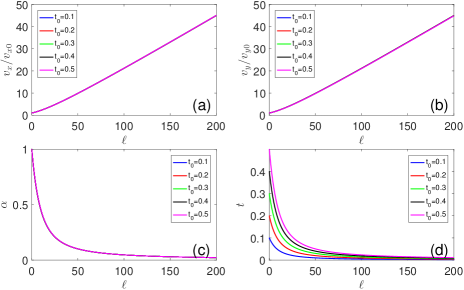
Figure 1: Flows of $v_{y}$, $v_{y}$, $\alpha$, and $t$ due to Coulomb interaction. Here, we assume $v_{y0}/v_{x0}=1$ and $\alpha_{0}=0.5$. The flavor $N=4$.

IV.2 Disorder effects

We next investigate the physical effect of disorders on the behavior of non-interacting tilted Dirac fermions. Under RG transformations, the disorder may be irrelevant, marginally irrelevant, marginal, and relevant as the running scale $\ell$ increases. For an irrelevant disorder, the effective strength flows to zero rapidly, and the low-energy properties of the system is not qualitatively changed by disorder scattering. For a marginally irrelevant disorder, the effective strength vanishes slowly, and the observable quantities acquire weak logarithmic-like corrections to their energy or temperature dependence. For a marginal disorder, the effective strength flows to a fixed point, and the observable quantities receives power-law corrections. For a relevant disorder, the effective strength increases indefinitely with growing $\ell$, and thus the system becomes unstable and should enter into a distinct phase. As demonstrated in extensive RG studies, relevant disorder can convert the SM into a CDM phase Ludwig94 ; Ostrovsky06 ; Evers08 ; Foster12 ; Goswami11 ; Nandkishore17 ; YuXuanWang17 ; WangLiuZhang17MWSM ; Mandal17 ; Sikkenk17 ; Roy14 ; Syzranov16 ; Roy16 ; Luo18 ; Roy18 , in which the fermions acquire a finite disorder scattering rate $\gamma_{0}$. In addition, the zero-energy fermion DOS $\rho(0)$ takes a finite value that is determined by $\gamma_{0}$. In contrast, $\rho(0)=0$ in the SM phase. Thus, the SM and CDM phases can be well distinguished by the value of $\gamma_{0}$ and $\rho(0)$. In this subsection, we present the detailed RG results for RSP, $x$-RVP, $y$-RVP, and RM, and analyze the unusual disorder-induced properties.

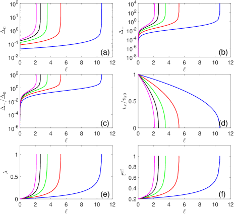
Figure 2: RG flows of $\Delta_{0}$, $\Delta_{-}$, $\Delta_{-}/\Delta_{0}$, and $t^{\mathrm{eff}}$ due to RSP. Blue, red, green, black, and magenta lines correspond to initial values $\Delta_{0,0}=0.04,0.08,0.12,0.16,0.2$, respectively. Here, $t_{0}=0.2$ and $v_{y0}/v_{x0}=1$.

IV.2.1 RSP

We first consider RSP. Its strength parameter $\Delta_{0}$ flows to infinity at a finite scale $\ell_{c}$, as showed by Fig. 2(a). A unique feature of RSP is that it always generates the fermion-disorder coupling term defined by Eq. (18) if the tilt parameter $t_{0}$ is nonzero. According to Fig. 2(b), the strength parameter $\Delta_{-}$ also diverges rapidly as $\ell\rightarrow\ell_{c}$. From Fig. 2(c), we observe that the ratio $\Delta_{-}/\Delta_{0}\rightarrow\infty$ as $\ell$ increases. This indicates that the dynamically generated disorder is much more important than RSP at low energies. The divergence of disorder strength parameters indicates that the tilted DSM becomes unstable and would be turned into a CDM in which both $\gamma_{0}$ and $\rho(0)$ are nonzero. The tilt parameter $t$ is fixed at its initial value, namely $t=t_{0}$. Interestingly, we find that $\lambda\rightarrow 1$ as $\ell$ grows as shown in Fig. 2(e). Consequently, the effective tilt parameter now becomes

$$t^{\mathrm{eff}}=\frac{t+\lambda}{1+t\lambda}\rightarrow\frac{t_{0}+1}{1+t_{0}}=1,$$ (53)

which is displayed in Fig. 2(f).

The eigenvalues of a Hamiltonian contain important information. For an interacting fermion system, the real part of the energy eigenvalues represents the energy dispersion of fermions, whereas the imaginary part characterizes the fermion damping effect. For a non-interacting 2D DSM, the real part of the energy vanishes at discrete points in the Brillouin zone, corresponding to the Dirac points, and the imaginary part is zero. Under certain circumstances, the real part of the energy may vanish along a finite curve in the Brillouin zone Kozii17 ; Papaj18 after incorporating the corrections due to disorder scattering, electron-electron scatting, or electron-phonon scattering. This curve is usually called a bulk Fermi arc, which has recently attracted considerable research interest Kozii17 ; Papaj18 ; Zhao18 .

We now examine whether RSP leads to a bulk Fermi arc in the system under consideration. Once finite disorder scattering rate $\gamma_{0}$ is generated in the CDM phase, the retarded fermion propagator can be written as

$$G^{R}(\omega,\mathbf{k})=\frac{1}{\omega+i\gamma_{0}-tv_{x}k_{x}-(\lambda\omega+it\gamma_{0})\sigma_{x}-v_{x}k_{x}\sigma_{x}-v_{y}k_{y}\sigma_{y}}.$$ (54)

The eigenvalues of disordered Hamiltonian are determined by

$$\left|\left|\left(E+i\gamma_{0}\right)-tv_{x}k_{x}-\left(\lambda E+it\gamma_{0}\right)\sigma_{x}-v_{x}k_{x}\sigma_{x}-v_{y}k_{y}\sigma_{y}\right|\right|=0,$$ (55)

which is equivalent to

$$\left|\begin{array}[]{cc}E+i\gamma_{0}-tv_{x}k_{x}&-\left(\lambda E+it\gamma_{0}\right)-v_{x}k_{x}-iv_{y}k_{y}\\ -\left(\lambda E+it\gamma_{0}\right)-v_{x}k_{x}+iv_{y}k_{y}&E+i\gamma_{0}-tv_{x}k_{x}\end{array}\right|=0.$$ (58)

The solution of this equation is

$$E_{\pm}(\mathbf{k})=\frac{\left(t+\lambda\right)v_{x}k_{x}-\left(1-t\lambda\right)i\gamma_{0}}{1-\lambda^{2}}\pm\sqrt{\frac{1}{\left(1-\lambda^{2}\right)^{2}}\left[\left(1+t\lambda\right)v_{x}k_{x}+\left(t-\lambda\right)i\gamma_{0}\right]^{2}+\frac{1}{1-\lambda^{2}}v_{y}^{2}k_{y}^{2}}.$$ (59)

If $\lambda$ flows to a fixed point $\lambda=t$, the scattering rate $\gamma_{0}$ does not induce bulk Fermi arc, but only represents fermion damping. However, our RG analysis shows that generically $\lambda\neq t$. Thus, for $k_{x}=0$,

$$E_{\pm}(\mathbf{k})=\frac{\left(t\lambda-1\right)i\gamma_{0}}{1-\lambda^{2}}\pm\sqrt{\frac{v_{y}^{2}k_{y}^{2}}{1-\lambda^{2}}-\gamma_{0}^{2}\left(\frac{t-\lambda}{1-\lambda^{2}}\right)^{2}}.$$ (60)

If $|k_{y}|<\frac{|t-\lambda|}{v_{y}\sqrt{1-\lambda^{2}}}\gamma_{0}$, the energy $E$ is pure imaginary. There emerges a bulk Fermi arc in the Brillouin zone Kozii17 ; Papaj18 , which replaces Dirac points. In this state, the fermion DOS, specific heat, and compressibility behave as $\rho(0)>0$, $C_{v}(T)\sim T$, and $\kappa(0)>0$. If the Dirac cone is not tilted, i.e., $t=0$, we always have $\lambda=\lambda_{0}=0$. Although RSP still leads to CDM transition in the untilted case, there is no bulk Fermi arc.

IV.2.2 $x$-RVP

In case $x$-RVP exists by itself, we plot the flows of $\Delta_{1}$, $\Delta_{-}$, $\Delta_{-}/\Delta_{1}$, $v_{x}$, $\lambda$, and $t$ in Figs. 3(a)-(f). The results are qualitatively the same as those shown in Fig. 2. The $x$-RVP also generates the new fermion-disorder coupling term Eq. (17), which then leads to a finite scattering rate $\gamma_{0}$ as well as a bulk Fermi arc.

We emphasize that the emergence of bulk Fermi arc induced by RSP or $x$-RVP is closely related to the presence of the term Eq. (17). If this term is naively discarded in the calculation, we would find that $\lambda$ always flows to the fixed point $\lambda=t$. In this case, no bulk Fermi arc emerges even though a finite $\gamma_{0}$ is generated. The detailed analysis is presented in Appendix D. Here, we briefly discuss the RG flow of $\lambda$. We already see from Figs. 2 and 3 that $\lambda\rightarrow 1$ and $t^{\mathrm{eff}}\rightarrow 1$ at certain scale $\ell_{c}$ due to RSP or $x$-RVP. The flow equation for $\lambda$ is

$$\frac{d\lambda}{dt} = \frac{1+t\lambda}{\left(1-t^{2}\right)^{3/2}}\left[\left(t-\lambda\right)\left(\Delta_{0}+\Delta_{1}\right)\right.$$ (61)

$$\left.+(1-t)\left(1-\lambda\right)\frac{\Delta_{-}}{2}\right].$$

Dropping disorder $\Delta_{-}$, this flow equation becomes

$$\frac{d\lambda}{dt}=\frac{1+t\lambda}{\left(1-t^{2}\right)^{3/2}}\left(t-\lambda\right)\left(\Delta_{0}+\Delta_{1}\right).$$ (62)

It is easy to see that $\lambda=t$ is a fixed point. thus $\lambda\rightarrow t$ if we ignore $\Delta_{-}$. If we choose to drop $\Delta_{0}$ and $\Delta_{1}$, the flow equation would become

$$\frac{d\lambda}{dt}=\frac{1+t\lambda}{\left(1-t^{2}\right)^{3/2}}\left(1-t\right)\left(1-\lambda\right)\frac{\Delta_{-}}{2}.$$ (63)

In this limit, $\lambda=1$ is a fixed point, and $\lambda\rightarrow 1$ as $\ell$ increases. Since $\Delta_{-}/\Delta_{0}\rightarrow\infty$ and $\Delta_{-}/\Delta_{1}\rightarrow\infty$, the dynamically generated disorder dominates over RSP and $x$-RVP in the low-energy region. Comparing to $\Delta_{-}$, $\Delta_{0}$ and $\Delta_{1}$ could be asymptotically neglected. Therefore, one can approximately replace Eq. (61) with Eq. (63). This is the reason why $\lambda\rightarrow 1$. Sikkenk and Fritz Sikkenk17 studied the disorder effects in tilted 3D WSM, and found that the parameter $\lambda\rightarrow 1$ as the disorder strength parameter flows to infinity. This is well consistent with our results obtained in tilted 2D DSM with RSP or $x$-RVP.

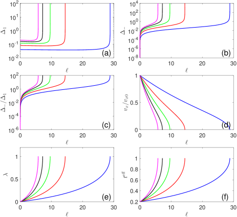
Figure 3: RG flows of $\Delta_{1}$, $\Delta_{-}$, $\Delta_{-}/\Delta_{1}$, and $t^{\mathrm{eff}}$ due to $x$-RVP. Blue, red, green, black, and magenta lines correspond to the initial values $\Delta_{1,0}=0.04,0.08,0.12,0.16,0.2$, respectively. Here, $t_{0}=0.2$ and $v_{y0}/v_{x0}=1$.

IV.2.3 $y$-RVP

The $x$- and $y$-components of RVP are equivalent in untilted systems. But they become distinct if the Dirac cone is tilted along $x$-axis. When $y$-RVP is added to tilted 2D DSM, it does not generate new disorder, and the corresponding RG equations are

$$\frac{dv_{x}}{d\ell} = -\frac{1+t\lambda}{\left(1-t^{2}\right)^{3/2}}\Delta_{2}v_{x},$$ (64)

$$\frac{dv_{y}}{d\ell} = -\frac{1+t\lambda}{\left(1-t^{2}\right)^{3/2}}\Delta_{2}v_{y},$$ (65)

$$\frac{d(v_{y}/v_{x})}{d\ell} = 0,$$ (66)

$$\frac{d(tv_{x})}{d\ell} = -\frac{1+t\lambda}{\left(1-t^{2}\right)^{3/2}}\Delta_{2}tv_{x},$$ (67)

$$\frac{dt}{d\ell} = 0,$$ (68)

$$\frac{d\lambda}{d\ell} = -\frac{\left(1+t\lambda\right)\left(\lambda+t\right)}{\left(1-t^{2}\right)^{3/2}}\Delta_{2},$$ (69)

$$\frac{d\Delta_{2}}{d\ell} = 0.$$ (70)

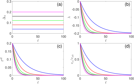
Figure 4: Flows of $\Delta_{2}$, $\lambda$, $t^{\mathrm{eff}}$, and $v_{x}$ due to $y$-RVP. Blue, red, green, black, and magenta lines correspond to the initial values $\Delta_{2,0}=0.04,0.08,0.12,0.16,0.2$, respectively. Here, $t_{0}=0.2$ and $v_{y0}/v_{x0}=1$.

The tilt $t$, velocity ratio $v_{y}/v_{x}$, and disorder strength $\Delta_{2}$ are all independent of $\ell$, and thus can be fixed at constants, namely $t=t_{0}$, $v_{y}/v_{x}=v_{y0}/v_{x0}$, and $\Delta_{2}=\Delta_{2,0}$. Then the RG equation for $\lambda$ becomes

$$\frac{d\lambda}{d\ell} = -\frac{\left(1+t_{0}\lambda\right)\left(\lambda+t_{0}\right)}{\left(1-t_{0}^{2}\right)^{3/2}}\Delta_{2,0}.$$ (71)

For initial value $\lambda_{0}=0$, $\lambda$ flows quickly to a stable fixed point $\lambda^{*}=-t_{0}$. In the lowest energy limit, the effective tilt parameter satisfies

$${t^{\mathrm{eff}}}^{*}=\frac{t_{0}+\lambda^{*}}{1+t_{0}\lambda^{*}}=0.$$ (72)

Thus $y$-RVP tends to suppress the tilt. The RG flows of $\Delta_{2}$, $\lambda$, $t^{\mathrm{eff}}$, and $v_{x}$ with varying $\ell$ are shown in Fig. 4.

In the low-energy region, the RG equations for $v_{x}$ and $v_{y}$ are approximately given by

$$\frac{dv_{x}}{d\ell} \sim -\frac{1+t_{0}\lambda^{*}}{\left(1-t_{0}^{2}\right)^{3/2}}\Delta_{2,0}v_{x}\sim-\eta_{0}v_{x},$$ (73)

$$\frac{dv_{y}}{d\ell} \sim -\frac{1+t_{0}\lambda^{*}}{\left(1-t_{0}^{2}\right)^{3/2}}\Delta_{2,0}v_{y}\sim-\eta_{0}v_{y},$$ (74)

where

$$\eta_{0}=\frac{\Delta_{2,0}}{\left(1-t_{0}^{2}\right)^{1/2}}.$$ (75)

The solutions of $v_{x}$ and $v_{y}$ are

$$v_{x}\sim v_{x0}e^{-\eta_{0}\ell},\qquad v_{y}\sim v_{y0}e^{-\eta_{0}\ell}.$$ (76)

It is clear that $v_{x}$ and $v_{y}$ approach to zero as $\ell\rightarrow\infty$. Employing the transformation $k=k_{0}e^{-\ell}$, where $k_{0}$ is taken as a fixed large value of $k$, we further express $v_{x}$ and $v_{y}$ as

$$v_{x}\sim v_{x0}\left(\frac{k}{k_{0}}\right)^{\eta_{0}},\qquad v_{y}\sim v_{y0}\left(\frac{k}{k_{0}}\right)^{\eta_{0}}.$$ (77)

The parameters $v_{x}^{\mathrm{eff}}$ and $v_{y}^{\mathrm{eff}}$ are given by

$$v_{x}^{\mathrm{eff}} \sim \frac{1+t_{0}\lambda^{*}}{1-{\lambda^{*}}^{2}}v_{x}\sim v_{x0}\left(\frac{k}{k_{0}}\right)^{\eta_{0}},$$ (78)

$$v_{y}^{\mathrm{eff}} \sim \frac{1}{\sqrt{1-{\lambda^{*}}^{2}}}v_{y}\sim\frac{1}{\sqrt{1-t_{0}^{2}}}v_{y0}\left(\frac{k}{k_{0}}\right)^{\eta_{0}}.$$ (79)

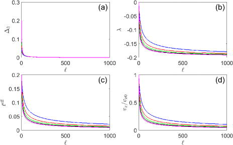
Figure 5: Flows of $\Delta_{3}$, $\lambda$, $t^{\mathrm{eff}}$, and $v_{x}$ due to RM. Blue, red, green, black, and magenta lines correspond to the initial values $\Delta_{3,0}=0.04,0.08,0.12,0.16,0.2$, respectively. Here, $t_{0}=0.2$ and $v_{y0}/v_{x0}=1$.

We notice that the dynamical exponent $z$ becomes $z=1+\eta_{0}$. Accordingly, the DOS depends on $\omega$ as follows

$$\rho(\omega)\sim\omega^{\frac{d}{z}-1}\sim\omega^{\frac{2}{1+\eta_{0}}-1}\sim\omega^{\frac{1-\eta_{0}}{1+\eta_{0}}}.$$ (80)

The specific heat and compressibility depend on $T$ as

$$C_{v}(T)\sim T^{\frac{d}{z}}\sim T^{\frac{2}{1+\eta_{0}}},$$ (81)

$$\kappa(T)\sim T^{\frac{d}{z}-1}\sim T^{\frac{1-\eta_{0}}{1+\eta_{0}}}.$$ (82)

These three quantities acquire power-law corrections. Comparing to the clean case, they are all enhanced by $y$-RVP. For a given $\Delta_{2,0}$, $\eta_{0}$ becomes larger with growing of $t_{0}$, as shown in Eq. (75), and the enhancement of DOS, specific heat, and compressibility is more significant. This indicates the influence of $y$-RVP is amplified by the tilt of Dirac cone.

IV.2.4 RM

Similar to $y$-RVP, RM also does not generate new disorders. The corresponding RG equations are

$$\frac{dv_{x}}{d\ell} = -\frac{1+t\lambda}{\left(1-t^{2}\right)^{3/2}}\Delta_{3}v_{x},$$ (83)

$$\frac{dv_{y}}{d\ell} = -\frac{1+t\lambda}{\left(1-t^{2}\right)^{3/2}}\Delta_{3}v_{y},$$ (84)

$$\frac{d(v_{y}/v_{x})}{d\ell} = 0,$$ (85)

$$\frac{d(tv_{x})}{d\ell} = -\frac{1+t\lambda}{\left(1-t^{2}\right)^{3/2}}\Delta_{3}tv_{x},$$ (86)

$$\frac{dt}{d\ell} = 0,$$ (87)

$$\frac{d\lambda}{d\ell} = -\frac{\left(1+t\lambda\right)\left(\lambda+t\right)}{\left(1-t^{2}\right)^{3/2}}\Delta_{3},$$ (88)

$$\frac{d\Delta_{3}}{d\ell} = -2\frac{1+t\lambda}{\left(1-t^{2}\right)^{3/2}}\Delta_{3}^{2}.$$ (89)

According to Eq. (85) and Eq. (87), we set $t=t_{0}$ and $v_{y}/v_{x}=v_{y0}/v_{x0}$. We solve the rest flow equations at initial value $\lambda=0$, and display the numerical results in Fig. 5. In the lowest energy limit, we find that

$$\lambda \rightarrow \lambda^{*}=-t_{0},$$ (90)

$$\Delta_{3} \rightarrow 0,$$ (91)

$${t^{\mathrm{eff}}}^{*} = \frac{t_{0}+\lambda^{*}}{1+t_{0}\lambda^{*}}=0.$$ (92)

Therefore, RM forces the tilted Dirac cone to go back to the untilted limit, in close analogy to the case of $y$-RVP. The RG equation for $\Delta_{3}$ is re-written as

$$\frac{d\Delta_{3}}{d\ell} \sim -2\frac{1}{\left(1-t_{0}^{2}\right)^{1/2}}\Delta_{3}^{2}.$$ (93)

Its solution is

$$\Delta_{3}\sim\frac{\Delta_{3,0}}{1+2\left(1-t_{0}^{2}\right)^{-1/2}\Delta_{3,0}\ell},$$ (94)

which approaches to zero slowly as $\ell\rightarrow\infty$.

In the low-energy region, one can approximate the RG equations for $v_{x}$ and $v_{y}$ by

$$\frac{dv_{x}}{d\ell} \sim -\frac{1+t_{0}\lambda^{*}}{\left(1-t_{0}^{2}\right)^{3/2}}\Delta_{3}v_{x}\sim-\frac{\Delta_{3}}{\left(1-t_{0}^{2}\right)^{1/2}}v_{x},$$ (95)

$$\frac{dv_{y}}{d\ell} \sim -\frac{1+t_{0}\lambda^{*}}{\left(1-t_{0}^{2}\right)^{3/2}}\Delta_{3}v_{y}\sim-\frac{\Delta_{3}}{\left(1-t_{0}^{2}\right)^{1/2}}v_{y}.$$ (96)

Substituting Eq. (94) into Eqs. (95) and (96), we find that $v_{x}$ and $v_{y}$ behave as

$$v_{x} \sim \frac{v_{x0}}{\sqrt{1+2\left(1-t_{0}^{2}\right)^{-3/2}\Delta_{3,0}\ell}},$$ (97)

$$v_{y} \sim \frac{v_{y0}}{\sqrt{1+2\left(1-t_{0}^{2}\right)^{-3/2}\Delta_{3,0}\ell}}.$$ (98)

Both $v_{x}$ and $v_{y}$ flow to zero slowly with growing $\ell$. Making use of the transformation $k=k_{0}e^{-\ell}$, we obtain

$$\frac{v_{x}}{v_{x0}}\sim\frac{v_{y}}{v_{y0}}\sim\frac{1}{\sqrt{1+2\left(1-t_{0}^{2}\right)^{-3/2}\Delta_{3,0}\ln\left(\frac{k_{0}}{k}\right)}}.$$ (99)

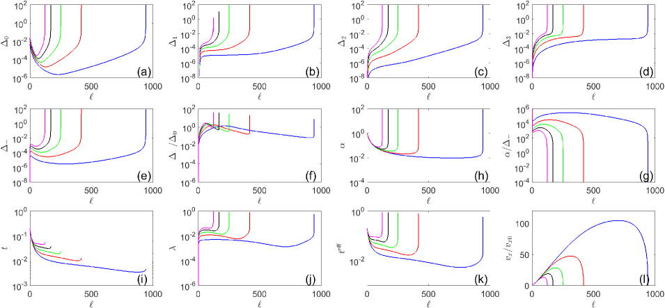
Figure 6: Flows of $\Delta_{0}$, $\Delta_{1}$, $\Delta_{2}$, $\Delta_{3}$, $\Delta_{-}$, $\Delta_{-}/\Delta_{0}$, $\alpha$, $\alpha/\Delta_{0}$, $t$, $\lambda$, $t^{\mathrm{eff}}$, and $v_{x}$ due to the interplay of RSP and Coulomb interaction. Blue, red, green, black, and magenta lines correspond to initial values $\Delta_{0,0}=0.005,0.01,0.015,0.02,0.025$, respectively. Here, $t_{0}=0.2$ and $v_{y0}/v_{x0}=1$. The flavor is $N=4$.

The parameters $v_{x}^{\mathrm{eff}}$ and $v_{y}^{\mathrm{eff}}$ are approximated as

$$v_{x}^{\mathrm{eff}} \sim \frac{1+t_{0}\lambda^{*}}{1-{\lambda^{*}}^{2}}v_{x}\sim v_{x},$$ (100)

$$v_{y}^{\mathrm{eff}} \sim \frac{1}{\sqrt{1-{\lambda^{*}}^{2}}}v_{y}\sim\frac{1}{\sqrt{1-t_{0}^{2}}}v_{y}.$$ (101)

We see that $v_{x}^{\mathrm{eff}}$ and $v_{y}^{\mathrm{eff}}$ exhibit the same momentum dependence as $v_{x}$ and $v_{y}$, respectively. In the clean limit, the DOS, specific heat, and compressibility depend on $\omega$ or $T$ as: $\rho(\omega)\sim\omega/(v_{x}^{\mathrm{eff}}v_{y}^{\mathrm{eff}})$, $C_{v}(T)\sim T^{2}/(v_{x}^{\mathrm{eff}}v_{y}^{\mathrm{eff}})$, and $\kappa(T)\sim T/(v_{x}^{\mathrm{eff}}v_{y}^{\mathrm{eff}})$. After considering the RM-induced corrections, these three quantities become

$$\rho(\omega) \sim \omega\ln\left(\frac{\omega_{0}}{\omega}\right),$$ (102)

$$C_{v}(T) \sim T^{2}\ln\left(\frac{T_{0}}{T}\right),$$ (103)

$$\kappa(T) \sim T\ln\left(\frac{T_{0}}{T}\right),$$ (104)

which display logarithmic corrections. Therefore, although RM and $y$-RVP both suppress tilt, they result in distinct low-energy properties of Dirac fermions.

IV.3 Interplay between interaction and disorder

The results of Sec. IV.2 are obtained in the non-interacting limit. We now turn to study the interplay between the Coulomb interaction and each single type of disorder, with the purpose of determining the physical consequence of Dirac cone tilt in realistic 2D DSMs.

IV.3.1 Coulomb interaction and RSP

When the Coulomb interaction and RSP are both present, they automatically generate all the other types of disorder, including $x$-RVP, $y$-RVP, RM, and the new disorder described by Eq. (18). As shown in Fig. 6, all the disorder strength parameters diverge at a finite scale $\ell_{c}$. The Coulomb interaction strength parameter $\alpha$ is also divergent at this scale, but the ratio $\alpha/\Delta_{i}$ vanishes. An apparent fact is that disorder always dominates over the Coulomb interaction at low energies, and determines the low-energy behaviors of the system. Consequently, there is always a finite disorder scattering rate and a bulk Fermi arc in the Brillouin zone.

The combination of Coulomb interaction and RSP has already been studied in the context of untilted 2D DSM Stauber05 ; WangLiu14 . While RSP is more important than weak Coulomb interaction and triggers the SM-to-CDM phase transition, a sufficiently strong Coulomb interaction can substantially suppress RSP and restore the original SM state. However, the SM state cannot be restored by the strong Coulomb interaction in tilted 2D DSM. It is therefore clear that the tilt does give rise to different properties than the untilted case.

IV.3.2 Coulomb interaction and $x$-RVP

Similar to RSP, the coexistence of Coulomb interaction and $x$-RVP also generates all the other types of disorder. The interaction strength $\alpha$ and the disorder parameters $\Delta_{i}$ also flow to the strong coupling regime, and their ratio $\alpha/\Delta_{i}$ still goes to zero. Thus, the system is inevitably turned into a CDM phase that features a finite scattering rate $\gamma_{0}$. Additionally, there also emerges a bulk Fermi arc. The model parameters depend on $\ell$ in qualitatively the same way as Fig. 6, and thus are not shown.

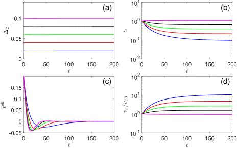
Figure 7: Flows of $\Delta_{2}$, $\lambda$, $t^{\mathrm{eff}}$, and $v_{x}$ due to the interplay between $y$-RVP and Coulomb interaction. Blue, red, green, black, and magenta lines correspond to initial values $\Delta_{2,0}=0.02,0.04,0.06,0.08,0.1$, respectively. Here, $t_{0}=0.2$, $v_{y0}/v_{x0}=1$, and $N=4$.

IV.3.3 Coulomb interaction and $y$-RVP

Coulomb interaction and $y$-RVP combine to yield

$$\frac{dv_{x}}{d\ell} = \left[\mathcal{H}_{1}(\alpha)-\frac{1+t\lambda}{\left(1-t^{2}\right)^{3/2}}\Delta_{2}\right]v_{x},$$ (105)

$$\frac{dv_{y}}{d\ell} = \left[\mathcal{H}_{2}(\alpha)-\frac{1+t\lambda}{\left(1-t^{2}\right)^{3/2}}\Delta_{2}\right]v_{y},$$ (106)

$$\frac{d(v_{y}/v_{x})}{d\ell} = \left[\mathcal{H}_{2}(\alpha)-\mathcal{H}_{1}(\alpha)\right]\frac{v_{y}}{v_{x}},$$ (107)

$$\frac{d(tv_{x})}{d\ell} = \left[-\frac{1+t\lambda}{\left(1-t^{2}\right)^{3/2}}\Delta_{2}t+\mathcal{H}_{3}(\alpha)\right]v_{x},$$ (108)

$$\frac{dt}{d\ell} = \mathcal{H}_{3}(\alpha)-\mathcal{H}_{1}(\alpha)t,$$ (109)

$$\frac{d\lambda}{d\ell} = -\frac{\left(1+t\lambda\right)\left(\lambda+t\right)}{\left(1-t^{2}\right)^{3/2}}\Delta_{2},$$ (110)

$$\frac{d\Delta_{2}}{d\ell} = \mathcal{H}_{6}(\alpha),$$ (111)

$$\frac{d\alpha}{d\ell} = \left[\frac{1+t\lambda}{\left(1-t^{2}\right)^{3/2}}\Delta_{2}-\frac{1}{2}\left(\mathcal{H}_{1}(\alpha)+\mathcal{H}_{2}(\alpha)\right)\right]\alpha.$$

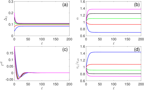
Figure 8: Flows of $\Delta_{3}$, $\lambda$, $t^{\mathrm{eff}}$, and $v_{x}$ due to the interplay between RM and Coulomb interaction. Blue, red, green, black, magenta lines correspond to the initial values $\Delta_{3,0}=0.04,0.08,0.12,0.16,0.2$, respectively. Here, $t_{0}=0.2$, $v_{y0}/v_{x0}=1$, and $N=4$.

The $\ell$-dependence of $\Delta_{2}$, $\alpha$, $t^{\mathrm{eff}}$, and $v_{x}$ can be found in Figs. 7(a)-(d). As $\ell$ grows, $\Delta_{2}$ and $\alpha$ approach to finite values $\Delta_{2}^{*}$ and $\alpha^{*}$, respectively. Thus the system is always in the stable quantum critical state characterized by $\Delta_{2}^{*}$ and $\alpha^{*}$. Coulomb interaction and $y$-RVP are both marginal. Fig. 7(c) shows that $t^{\mathrm{eff}}\rightarrow 0$, thus the tilt is suppressed. We see from Fig. 7(d) that, $v_{x}$ flows to a finite values $v_{x}^{*}$. $v_{y}$ also approaches to a finite value $v_{y}^{*}$, which is not shown here.

The $\ell$-dependence of fermion velocities indicates that the dynamical exponent recovers the value $z=1$. But the fermion field acquires a finite anomalous dimension

$$\eta_{\psi}=\frac{\Delta_{2}^{*}}{2\pi v_{x}^{*}v_{y}^{*}}.$$ (113)

Based on these results, we get the fermion DOS

$$\rho(\omega)\sim\omega^{1+\eta_{\psi}}.$$ (114)

The specific heat and compressibility exhibit the same behaviors as the non-interacting case, namely $C_{v}(T)\sim T^{2}$ and $\kappa(T)\sim T$. As shown in Appendix C, although the anomalous dimension $\eta_{\psi}$ is nonzero, it only modifies the coefficients, leaving the $T$-dependence unchanged.

Table 1: Summary of the flow behaviors of $t$, $\lambda$, $t^{\mathrm{eff}}$, $\alpha$, and disorder strength parameters in the low-energy region. The critical scale $\ell_{c}$ is always finite, but its precise value is case dependent.

Initial Condition	$\ell$	$t$	$\lambda$	$t^{\mathrm{eff}}=\frac{t+\lambda}{1+t\lambda}$	Disorder strength	$\alpha$
$\Delta_{0,0}>0$	when $\ell\rightarrow\ell_{c}$	$t=t_{0}$	$\lambda\rightarrow 1$	$t^{\mathrm{eff}}\rightarrow 1$	$\Delta_{0}\rightarrow\infty$ $\Delta_{-}\rightarrow\infty$ $\Delta_{-}/\Delta_{0}\rightarrow\infty$	-
$\Delta_{1,0}>0$	when $\ell\rightarrow\ell_{c}$	$t=t_{0}$	$\lambda\rightarrow 1$	$t^{\mathrm{eff}}\rightarrow 1$	$\Delta_{1}\rightarrow\infty$ $\Delta_{-}\rightarrow\infty$ $\Delta_{-}/\Delta_{1}\rightarrow\infty$	-
$\Delta_{2,0}>0$	when $\ell\rightarrow\infty$	$t=t_{0}$	$\lambda\rightarrow-t_{0}$	$t^{\mathrm{eff}}\rightarrow 0$	$\Delta_{2}=\Delta_{2,0}$	-
$\Delta_{3,0}>0$	when $\ell\rightarrow\infty$	$t=t_{0}$	$\lambda\rightarrow-t_{0}$	$t^{\mathrm{eff}}\rightarrow 0$	$\Delta_{3}\rightarrow 0$	-
$\alpha_{0}>0$	when $\ell\rightarrow\infty$	$t\rightarrow 0$	$\lambda=0$	$t^{\mathrm{eff}}\rightarrow 0$	-	$\alpha\rightarrow 0$
$\alpha_{0}>0$, $\Delta_{0,0}>0$	when $\ell\rightarrow\ell_{c}$	$t\rightarrow t^{*}$	$\lambda\rightarrow 1$	$t^{\mathrm{eff}}\rightarrow 1$	$\Delta_{0}\rightarrow\infty$ $\Delta_{-}\rightarrow\infty$ $\Delta_{-}/\Delta_{0}\rightarrow\infty$	$\alpha\rightarrow\infty$ $\alpha/\Delta_{-}\rightarrow 0$
$\alpha_{0}>0$, $\Delta_{1,0}>0$	when $\ell\rightarrow\ell_{c}$	$t\rightarrow t^{*}$	$\lambda\rightarrow 1$	$t^{\mathrm{eff}}\rightarrow 1$	$\Delta_{1}\rightarrow\infty$ $\Delta_{-}\rightarrow\infty$ $\Delta_{-}/\Delta_{1}\rightarrow\infty$	$\alpha\rightarrow\infty$ $\alpha/\Delta_{-}\rightarrow 0$
$\alpha_{0}>0$, $\Delta_{2,0}>0$	when $\ell\rightarrow\infty$	$t\rightarrow 0$	$\lambda\rightarrow 0$	$t^{\mathrm{eff}}\rightarrow 0$	$\Delta_{2}\rightarrow\Delta_{2}^{*}$	$\alpha\rightarrow\alpha^{*}$
$\alpha_{0}>0$, $\Delta_{3,0}>0$	when $\ell\rightarrow\infty$	$t\rightarrow 0$	$\lambda\rightarrow 0$	$t^{\mathrm{eff}}\rightarrow 0$	$\Delta_{3}\rightarrow\Delta_{3}^{*}$	$\alpha\rightarrow\alpha^{*}$

IV.3.4 Coulomb interaction and RM

Coulomb interaction and RM give rise to

$$\frac{dv_{x}}{d\ell} = \left[\mathcal{H}_{1}(\alpha)-\frac{1+t\lambda}{\left(1-t^{2}\right)^{3/2}}\Delta_{3}\right]v_{x},$$ (115)

$$\frac{dv_{y}}{d\ell} = \left[\mathcal{H}_{2}(\alpha)-\frac{1+t\lambda}{\left(1-t^{2}\right)^{3/2}}\Delta_{3}\right]v_{y},$$ (116)

$$\frac{d(v_{y}/v_{x})}{d\ell} = \left[\mathcal{H}_{2}(\alpha)-\mathcal{H}_{1}(\alpha)\right]\frac{v_{y}}{v_{x}},$$ (117)

$$\frac{d(tv_{x})}{d\ell} = \left[-\frac{1+t\lambda}{\left(1-t^{2}\right)^{3/2}}\Delta_{3}t+\mathcal{H}_{3}(\alpha)\right]v_{x},$$ (118)

$$\frac{dt}{d\ell} = \mathcal{H}_{3}(\alpha)-\mathcal{H}_{1}(\alpha)t,$$ (119)

$$\frac{d\Delta_{3}}{d\ell} = \left[-2\frac{1+t\lambda}{\left(1-t^{2}\right)^{3/2}}\Delta_{3}+\mathcal{H}_{7}(\alpha)\right]\Delta_{3},$$ (120)

$$\frac{d\alpha}{d\ell} = \left[\frac{1+t\lambda}{\left(1-t^{2}\right)^{3/2}}\Delta_{3}-\frac{1}{2}\left(\mathcal{H}_{1}(\alpha)+\mathcal{H}_{2}(\alpha)\right)\right]\alpha.$$

As illustrated by Figs. 8(a) and (b), $\Delta_{3}\rightarrow\Delta_{3}^{*}$ and $\alpha\rightarrow\alpha^{*}$, where $\Delta_{3}^{*}$ and $\alpha^{*}$ are two constants. The effective tilt parameter $t^{\mathrm{eff}}\rightarrow 0$, and $v_{x}\rightarrow v_{x}^{*}$ in the lowest energy limit, which can be easily seen from Figs. 8(c) and (d).

The system also flows to a stable quantum critical state in which the dynamical exponent $z=1$ and the fermion anomalous dimension

$$\eta_{\psi}=\frac{\Delta_{3}^{*}}{2\pi v_{x}^{*}v_{y}^{*}}.$$ (122)

These results are qualitatively very similar to those induced by the interplay between Coulomb interaction and $y$-RVP. Once again, the DOS $\rho(\omega)\sim\omega^{1+\eta_{\psi}}$, the specific heat $C_{v}(T)\sim T^{2}$, and the compressibility $\kappa(T)\sim T$.

V Summary and Discussion

In summary, we have studied the physical effects of Dirac cone tilt on the low-energy behaviors of 2D DSM by performing a RG analysis of the interplay between Coulomb interaction and quenched disorder. For the tilt along $x$-axis, there are generically four types of disorder: RSP, $x$-RVP, $y$-RVP, and RM. We find that RSP and $x$-RVP are distinct from $y$-RVP and RM. As long as the tilt is finite, RSP cannot exist on its own and its coupling to the Dirac fermions inevitably generates a new type of disorder. The dynamically generated disorder plays the dominant role in the low-energy region, and drives an SM-to-CDM quantum phase transition. As the result, the fermions acquire a finite disorder scattering rate. Moreover, the originally isolated Dirac points are replaced by a bulk Fermi arc. We also find that $x$-RVP leads to nearly the same low-energy behaviors as RSP. These results are not altered when the Coulomb interaction is incorporated. Different from RSP and $x$-RVP, $y$-RVP or RM can exist alone without generating other types of disorder. In addition, both $y$-RVP and RM tend to suppress the Dirac cone tilt. When the Coulomb interaction and $y$-RVP (or RM) exist concomitantly, they cooperate to produce a stable quantum critical state, in which the dynamical exponent $z=1$ and the fermion anomalous dimension is nonzero. All these results are summarized in Table 1. To characterize the low-energy behaviors, we also calculate the fermion DOS, specific heat, and compressibility in various conditions, and summarize the results in Table 2.

Table 2: Summary of low-energy or low-temperature properties of some observable quantities, including DOS, specific heat, and compressibility, obtained in different conditions.

Initial Condition	DOS $\rho(\omega)$	Specific heat $C_{v}(T)$	Compressibility $\kappa(T)$
Clean and Free	$\rho(\omega)\sim\omega$	$C_{v}(T)\sim T^{2}$	$\kappa(T)\sim T$
$\Delta_{0,0}>0$	$\rho(0)>0$	$C_{v}(T)\sim\rho(0)T$	$\kappa(0)>0$
$\Delta_{1,0}>0$	$\rho(0)>0$	$C_{v}(T)\sim\rho(0)T$	$\kappa(0)>0$
$\Delta_{2,0}>0$	$\rho(\omega)\sim\omega^{(1-\eta_{0})/(1+\eta_{0})}$	$C_{v}(T)\sim T^{2/(1+\eta_{0})}$	$\kappa(T)\sim T^{(1-\eta_{0})/(1+\eta_{0})}$
$\Delta_{3,0}>0$	$\rho(\omega)\sim\omega\ln\left(\omega_{0}/\omega\right)$	$C_{v}(T)\sim T^{2}\ln(T_{0}/T)$	$\kappa(T)\sim T\ln(T_{0}/T)$
$\alpha_{0}>0$	$\rho(\omega)\sim\omega/\ln^{2}(\omega_{0}/\omega)$	$C_{v}(T)\sim T^{2}/\ln^{2}(T_{0}/T)$	$\kappa(T)\sim T/\ln^{2}(T_{0}/T)$
$\alpha_{0}>0$, $\Delta_{0,0}>0$	$\rho(0)>0$	$C_{v}(T)\sim\rho(0)T$	$\kappa(0)>0$
$\alpha_{0}>0$, $\Delta_{1,0}>0$	$\rho(0)>0$	$C_{v}(T)\sim\rho(0)T$	$\kappa(0)>0$
$\alpha_{0}>0$, $\Delta_{2,0}>0$	$\rho(\omega)\sim\omega^{1+\eta_{\psi}(\Delta_{2}^{*})}$	$C_{v}(T)\sim T^{2}$	$\kappa(T)\sim T$
$\alpha_{0}>0$, $\Delta_{3,0}>0$	$\rho(\omega)\sim\omega^{1+\eta_{\psi}(\Delta_{3}^{*})}$	$C_{v}(T)\sim T^{2}$	$\kappa(T)\sim T$

It is useful to highlight the unusual effects caused by the tilt. For untilted 2D DSM, previous studies Ludwig94 ; Ostrovsky06 ; Evers08 ; Foster12 have already confirmed that any of the four types of disorder can individually exist. More concretely, RSP is relevant and converts the DSM into a CDM, in which the fermions have finite disorder scattering rate but no bulk Fermi arc appears. The two components of RVP, namely $x$-RVP and $y$-RVP, are equivalent: they are marginal and lead to stable quantum critical state characterized by power-law corrections to observable quantities. RM is marginally irrelevant and merely causes weak logarithmic-like corrections to observable quantities. When the Dirac cone is tilted along $x$-axis, $x$-RVP becomes entirely different from $y$-RVP. In fact, $x$-RVP gives rise to nearly the same physical consequences as RSP: they always dynamically generate a new type of disorder, and induce a bulk Fermi arc. In the case of zero tilt, these two features are both absent. In contrast, $y$-RVP or RM leads to nearly the same low-energy properties in 2D tilted DSM as those of the untilted case.

The interplay of Coulomb interaction and disorder in untilted 2D DSM has also been studied extensively Ye98 ; Ye99 ; Stauber05 ; Herbut08 ; Vafek08 ; Foster08 ; WangLiu14 . If Coulomb interaction and RVP are both considered, 2D DSM is driven to enter into a stable quantum critical state, in which the fermion field acquires a finite anomalous dimension but the dynamical exponent becomes $z=1$ Ye98 ; Ye99 ; Stauber05 ; Herbut08 ; Vafek08 ; Foster08 ; WangLiu14 . Coexistence of Coulomb interaction and RM leads to similar stable quantum critical state Ye98 ; Ye99 ; Stauber05 ; Foster08 ; WangLiu14 . The behaviors induced by $y$-RVP and RM are not qualitatively altered by the tilt. Actually, tilt mainly changes the physical effects of RSP and $x$-RVP.

Sikkenk and Fritz Sikkenk17 studied the disorder effects on 3D WSM tilted along a generic direction. They found that RSP and RVP can exist individually in untilted system but always generate each other at finite tilt. This is similar to the result obtained in this work. For weak RSP and RVP, their strength parameters both flow to zero in the lowest energy limit. However, both RSP and RVP flow to the strong coupling regime if the initial strength is large enough, which generates a finite scattering rate. In the latter case, there should also emerge a bulk Fermi arc, although this conclusion was not noticed in Ref. Sikkenk17 . In Ref. Detassis17 , Detassis et al. considered the effects caused by the Coulomb interaction on tilted 3D DSM/WSM, and showed that the tilt is completely suppressed by the Coulomb interaction, consistent with the result obtain in the context of tilted 2D DSM Isobe12 ; LeeLee18 . Pozo et al. Pozo18 analyzed the influence of the electromagnetic field on 3D DSM/WSM with finite tilt, and found that the tilt parameter approaches to a finite value in the lowest energy limit when the polarization of photon is properly taken into account.

Recently, Papaj and Fu Papaj18 investigated disorder effects in a model in which the Dirac fermions come from two distinct orbitals. In this model, disorder acts on two orbitals differently. They showed Papaj18 that a finite tilt is generated naturally due to the orbit-dependent disorder scattering even when the Dirac cone is initially not tilted. Because two orbitals acquire different disorder scattering rates, the original Dirac points are replaced by a bulk Fermi arc Papaj18 . Later, Zhao et al. Zhao18 extended the analysis of Papaj and Fu Papaj18 to the more generic case in which several types of disorder coexist, and obtained a condition for the Fermi arc to emerge. The model considered in our work differs from the one studied in Refs. Papaj18 ; Zhao18 in that the two components of the spinor field have different physical origin. According to our results, both RSP and $x$-RVP can dynamically generate a new type of disorder, which then plays an overwhelming role at low energies. The striking phenomenon of dynamical disorder generation was not considered in Refs. Papaj18 ; Zhao18 .

Appendix A Deriving RG equations

Here we present the detailed derivation of the coupled RG equations for all the involved model parameters.

A.1 Self-energy corrections of fermions

The fermion self-energy stems from two interactions: Coulomb interaction and disorder scattering. We consider two cases in order.

A.1.1 Self-energy induced by Coulomb interaction

The self-energy of fermions induced by the long-range Coulomb interaction is defined as

$$\Sigma^{C}(i\omega,\mathbf{k}) = -\int^{\prime}\frac{d\Omega}{2\pi}\frac{d^{2}\mathbf{q}}{(2\pi)^{2}}G_{0}\left(i\omega+i\Omega,\mathbf{k}+\mathbf{q}\right)$$ (123)

$$\times D(\mathbf{q}),$$

where $\int^{\prime}$ means that the integration requires a proper choice of the momentum shell. We choose to integrate in the ranges of $-\infty<\Omega<\infty$ and $b\Lambda<E_{\mathbf{k}}<\Lambda$, where $E_{\mathbf{k}}=tv_{x}k_{x}+\sqrt{v_{x}^{2}k_{x}^{2}+v_{y}^{2}k_{y}^{2}}$ and $b=e^{-\ell}$. Substituting Eqs. (6) and (10) into Eq. (123) and expanding up to the leading order, we obtain

$$\Sigma^{C}(i\omega,\mathbf{k})\approx\left[\Sigma^{C}_{t}v_{x}k_{x}+\Sigma^{C}_{x}v_{x}k_{x}\sigma_{x}+\Sigma^{C}_{y}v_{y}k_{y}\sigma_{y}\right]\ell,$$ (124)

where

$$\Sigma^{C}_{t} = \lambda\left(1+t\lambda\right)f_{A}(\alpha),$$ (125)

$$\Sigma^{C}_{x} = \left(1+t\lambda\right)f_{A}(\alpha),$$ (126)

$$\Sigma^{C}_{y} = \left(1+t\lambda\right)^{2}f_{B}(\alpha),$$ (127)

where $f_{A}$ and $f_{B}$ are given by Eqs. (42) and (43).

Figure 9: Diagrams of vertex corrections to fermion-disorder coupling. Solid, dashed, and wave lines represent fermion propagator, disorder scattering, and Coulomb interaction.

A.1.2 Self-energy induced by disorder scattering

The fermion self-energy caused by disorder scattering is given by

$$\Sigma^{\mathrm{dis}}(i\omega)=\sum_{n}\Delta_{n}\int^{\prime}\frac{d^{2}\mathbf{p}}{(2\pi)^{2}}\Gamma_{n}G_{0}\left(i\omega,\mathbf{p}\right)\Gamma_{n},$$ (128)

where $\sum_{n}\equiv\sum_{n=0,1,2,3,-}$. Substituting Eq. (10) into Eq. (128) and retaining the leading order contribution, we get

$$\Sigma^{\mathrm{dis}}(i\omega) \approx \left(i\omega\Sigma^{\mathrm{dis}}_{\omega}\sigma_{0}+i\omega\Sigma^{\mathrm{dis}}_{\lambda}\sigma_{x}\right)\ell,$$ (129)

where

$$\Sigma^{\mathrm{dis}}_{\omega} = -\left[\left(\Delta_{0}+\Delta_{1}+\Delta_{2}+\Delta_{3}\right)+(1+t)\frac{\Delta_{-}}{2}\right]$$ (130)

$$\times\frac{1+t\lambda}{2\pi v_{x}v_{y}\left(1-t^{2}\right)^{3/2}},$$

$$\Sigma^{\mathrm{dis}}_{\lambda} = \left[t\left(\Delta_{0}+\Delta_{1}-\Delta_{2}-\Delta_{3}\right)+\left(1+t\right)\frac{\Delta_{-}}{2}\right]$$ (131)

$$\times\frac{1+t\lambda}{2\pi v_{x}v_{y}\left(1-t^{2}\right)^{3/2}}.$$

A.2 Corrections to fermion-disorder coupling

Diagram 9(a) represents the correction to the fermion-disorder coupling induced by Coulomb interaction. We have

$$W^{a} = \sum_{n}W_{n}^{a},$$ (132)

$$W_{n}^{a} = -\Delta_{n}\int^{\prime}\frac{d\Omega}{2\pi}\frac{d^{2}\mathbf{q}}{(2\pi)^{2}}\left(\psi^{{\dagger}}G_{0}\left(i\Omega,\mathbf{q}\right)\Gamma_{n}G_{0}\left(i\Omega,\mathbf{q}\right)\psi\right)$$ (133)

$$\times\left(\psi^{{\dagger}}\Gamma_{n}\psi\right)D(\mathbf{q}).$$

After tedious but straightforward calculations, we finally obtain

$$W^{a}=\left[\sum_{n}\delta\Delta_{n}^{a}\left(\psi^{{\dagger}}\Gamma_{n}\psi\right)\left(\psi^{{\dagger}}\Gamma_{n}\psi\right)\right]\ell,$$ (134)

where

$$\delta\Delta_{0}^{a} = \left[\lambda\left(1+2\lambda\right)\Delta_{0}+\lambda\Delta_{1}-\frac{1}{4}\left(1-\lambda^{2}\right)\Delta_{-}\right]$$ (135)

$$\times\frac{f_{A}(\alpha)}{2\left(1-\lambda^{2}\right)^{3/2}},$$

$$\delta\Delta_{1}^{a} = \left[\lambda\Delta_{0}+\left(2+\lambda\right)\Delta_{1}+\frac{1}{4}\left(1-\lambda^{2}\right)\Delta_{-}\right]$$ (136)

$$\times\frac{f_{A}(\alpha)}{2\left(1-\lambda^{2}\right)^{3/2}},$$

$$\delta\Delta_{2}^{a} = \left(1+t\lambda\right)^{2}\Delta_{2}\frac{f_{B}(\alpha)}{\left(1-\lambda^{2}\right)^{3/2}},$$ (137)

$$\delta\Delta_{3}^{a} = \left[\left(1-\lambda^{2}\right)f_{A}(\alpha)+\left(1+t\lambda\right)^{2}f_{B}(\alpha)\right]$$ (138)

$$\times\frac{\Delta_{3}}{\left(1-\lambda^{2}\right)^{3/2}},$$

$$\delta\Delta_{-}^{a} = \left[-4\lambda\left(\Delta_{0}+\Delta_{1}\right)+\left(1+\lambda\right)^{2}\Delta_{-}\right]$$ (139)

$$\times\frac{f_{A}(\alpha)}{2\left(1-\lambda^{2}\right)^{3/2}}.$$

In the derivation of these equations, we have encountered a new coupling term $\left(\psi^{{\dagger}}\sigma_{x}\psi\right)\left(\psi^{{\dagger}}\sigma_{0}\psi\right)$, which does not exist in the starting action but is generated by fermion-disorder interaction. To deal with this new term, we find it convenient to decouple it as follows

$$\left(\psi^{{\dagger}}\sigma_{x}\psi\right)\left(\psi^{{\dagger}}\sigma_{0}\psi\right) = -2\left(\psi^{{\dagger}}\sigma_{-}\psi\right)\left(\psi^{{\dagger}}\sigma_{-}\psi\right)$$ (140)

$$+\frac{1}{2}\left(\psi^{{\dagger}}\sigma_{0}\psi\right)\left(\psi^{{\dagger}}\sigma_{0}\psi\right)$$

$$+\frac{1}{2}\left(\psi^{{\dagger}}\sigma_{x}\psi\right)\left(\psi^{{\dagger}}\sigma_{x}\psi\right).$$

Thus the dynamically generated term is actually a combination of RSP, $x$-RVP, and a new type of disorder defined by the matrix $\sigma_{-}$. Relation (140) is also employed in the following if the term $\left(\psi^{{\dagger}}\sigma_{x}\psi\right)\left(\psi^{{\dagger}}\sigma_{0}\psi\right)$ appears.

The contribution for the fermion-disorder coupling from the Feynman diagram 9(b) is given by

$$W^{b} = \sum_{n}W_{n}^{b},$$ (141)

$$W_{n}^{b} = \sum_{m}\int^{\prime}\frac{d^{2}\mathbf{p}}{(2\pi)^{2}}\left(\psi^{{\dagger}}\sigma_{m}G_{0}(0,\mathbf{p})\sigma_{n}G_{0}\left(0,\mathbf{p}\right)\sigma_{m}\psi\right)$$ (142)

$$\times\left(\psi^{{\dagger}}\sigma_{n}\psi\right).$$

Substituting Eq. (10) into Eqs. (141) and (142) and performing the calculation directly, we obtain

$$W^{b} = \left[\sum_{n}\delta\Delta_{n}^{b}\left(\psi^{{\dagger}}\Gamma_{n}\psi\right)\left(\psi^{{\dagger}}\Gamma_{n}\psi\right)\right]\ell,$$ (143)

where

$$\delta\Delta_{0}^{b} = \Bigg{[}\left(1-\frac{t}{2}\right)\Delta_{0}^{2}+\left(1-t\right)\Delta_{0}\Delta_{1}+\left(1+\frac{t}{2}\right)\Delta_{0}\Delta_{2}+\left(1+\frac{t}{2}\right)\Delta_{0}\Delta_{3}-\frac{t}{2}\Delta_{1}^{2}-\frac{t}{2}\Delta_{1}\Delta_{2}-\frac{t}{2}\Delta_{1}\Delta_{3}$$

$$+\left(\frac{3}{8}+\frac{t}{4}-\frac{t^{2}}{8}\right)\Delta_{0}\Delta_{-}+\left(\frac{1}{8}-\frac{t}{4}-\frac{3t^{2}}{8}\right)\Delta_{1}\Delta_{-}+\frac{\left(1+t\right)^{2}}{8}\left(\Delta_{2}+\Delta_{3}\right)\Delta_{-}\Bigg{]}\frac{1}{2\pi v_{x}v_{y}\left(1-t^{2}\right)^{3/2}},$$

$$\delta\Delta_{1}^{b} = \Bigg{[}-\frac{t}{2}\Delta_{0}^{2}-t\left(1-t\right)\Delta_{0}\Delta_{1}+\frac{t}{2}\Delta_{0}\Delta_{2}+\frac{t}{2}\Delta_{0}\Delta_{3}-t\left(\frac{1}{2}-t\right)\Delta_{1}^{2}-t\left(\frac{1}{2}+t\right)\Delta_{1}\left(\Delta_{2}+\Delta_{3}\right)$$

$$-\left(\frac{3}{8}+\frac{t}{4}-\frac{t^{2}}{8}\right)\Delta_{0}\Delta_{-}-\left(\frac{1}{8}-\frac{t}{4}-\frac{3t^{2}}{8}\right)\Delta_{1}\Delta_{-}-\frac{\left(1+t\right)^{2}}{8}\left(\Delta_{2}+\Delta_{3}\right)\Delta_{-}\Bigg{]}\frac{1}{2\pi v_{x}v_{y}\left(1-t^{2}\right)^{3/2}},$$

$$\delta\Delta_{2}^{b} = 0,$$ (146)

$$\delta\Delta_{3}^{b} = -\left(1-t^{2}\right)\left(\Delta_{0}-\Delta_{1}-\Delta_{2}+\Delta_{3}\right)\frac{1}{2\pi v_{x}v_{y}\left(1-t^{2}\right)^{3/2}},$$ (147)

$$\delta\Delta_{-}^{b} = \Bigg{[}2t\left(\Delta_{0}^{2}+2\Delta_{0}\Delta_{1}-\Delta_{0}\Delta_{2}-\Delta_{0}\Delta_{3}+\Delta_{1}^{2}+\Delta_{1}\Delta_{2}+\Delta_{1}\Delta_{3}\right)+\frac{1}{2}\left(3+4t+t^{2}\right)\Delta_{0}\Delta_{-}$$ (148)

$$+\frac{1}{2}\left(1+4t+3t^{2}\right)\Delta_{1}\Delta_{-}+\frac{1-t^{2}}{2}\left(\Delta_{2}+\Delta_{3}\right)\Delta_{-}+\frac{\left(1+t\right)^{2}}{2}\Delta_{-}^{2}\Bigg{]}\frac{1}{2\pi v_{x}v_{y}\left(1-t^{2}\right)^{3/2}}.$$

Diagram 9 (c) and diagram 9 (d) give rise to the following contributions to the fermion-disorder coupling vertex

$$W^{c+d} = \sum_{n}\sum_{m\leq n}W_{mn}^{c+d},$$ (149)

$$W_{mn}^{c+d} = \Delta_{m}\Delta_{n}\int^{\prime}\frac{d^{2}\mathbf{p}}{(2\pi)^{2}}\left(\psi^{{\dagger}}\Gamma_{m}G_{0}(0,\mathbf{p})\Gamma_{n}(0,\mathbf{p})\psi\right)\left(\psi^{{\dagger}}\left(\Gamma_{n}G_{0}(0,\mathbf{p})\Gamma_{m}+\Gamma_{m}G_{0}(0,-\mathbf{p})\Gamma_{n}\right)\psi\right).$$ (150)

Substituting Eq. (10) into Eqs. (149) and (150), we get

$$W^{c+d}=\left[\sum_{n}\delta\Delta_{n}^{c+d}\left(\psi^{{\dagger}}\Gamma_{n}\psi\right)\left(\psi^{{\dagger}}\Gamma_{n}\psi\right)\right]\ell,$$ (151)

where

$$\delta\Delta_{0}^{c+d} = \left[\left(1-t^{2}\right)\Delta_{1}+\left(1+t\right)\Delta_{2}\right]\frac{\Delta_{3}}{\pi v_{x}v_{y}\left(1-t^{2}\right)^{3/2}},$$ (153)

$$\delta\Delta_{1}^{c+d} = \left[\left(1-t^{2}\right)\Delta_{0}+t\left(1+t\right)\Delta_{2}\right]\frac{\Delta_{3}}{\pi v_{x}v_{y}\left(1-t^{2}\right)^{3/2}},$$ (154)

$$\delta\Delta_{2}^{c+d} = \left[\left(\Delta_{0}+t^{2}\Delta_{1}\right)+\frac{\left(1+t\right)^{2}\Delta_{-}}{4}\right]\frac{\Delta_{3}}{\pi v_{x}v_{y}\left(1-t^{2}\right)^{3/2}},$$ (155)

$$\delta\Delta_{3}^{c+d} = \Big{[}\left(1-t^{2}\right)\Delta_{0}\Delta_{1}+\Delta_{0}\Delta_{2}+t^{2}\Delta_{1}\Delta_{2}+\frac{1-t^{2}}{4}\left(\Delta_{0}+\Delta_{1}\right)\Delta_{-}+\frac{\left(1+t\right)^{2}}{4}\Delta_{2}\Delta_{+}\Big{]}\frac{1}{\pi v_{x}v_{y}\left(1-t^{2}\right)^{3/2}},$$

$$\delta\Delta_{-}^{c+d} = \left[-4t\Delta_{2}+\left(1-t^{2}\right)\Delta_{-}\right]\frac{\Delta_{3}}{\pi v_{x}v_{y}\left(1-t^{2}\right)^{3/2}}.$$ (157)

A.3 RG analysis

The original action of fermions is

$$S_{f} = \int\frac{d\omega}{2\pi}\frac{d^{2}\mathbf{k}}{(2\pi)^{2}}\psi^{{\dagger}}(\omega,\mathbf{k})\left[i\omega\sigma_{0}-i\lambda\omega\sigma_{x}\right.$$ (158)

$$\left.-\left(t\sigma_{0}+\sigma_{x}\right)v_{x}k_{x}-v_{y}k_{y}\sigma_{y}\right]\psi(\omega,\mathbf{k}).$$

The original action for fermion-disorder coupling has the form

$$S_{dis} = \sum_{n}\frac{\Delta_{n}}{2}\int\frac{d\omega_{1}d\omega_{2}d^{2}\mathbf{k}_{1}d^{2}\mathbf{k}_{2}d^{2}\mathbf{k}_{3}}{(2\pi)^{8}}$$ (159)

$$\times\left(\psi^{{\dagger}}(\omega_{1},\mathbf{k}_{1})\Gamma_{n}\psi(\omega_{1},\mathbf{k}_{2})\right)\left(\psi^{{\dagger}}(\omega_{2},\mathbf{k}_{3})\Gamma_{n}\right.$$

$$\left.\times\psi(\omega_{2},-\mathbf{k}_{1}-\mathbf{k}_{2}-\mathbf{k}_{3})\right),$$

where $n=0,1,2,3,-$. Including the corrections obtained in the last subsections leads to

$$S_{f}^{\prime} = \int\frac{d\omega}{2\pi}\frac{d^{2}\mathbf{k}}{(2\pi)^{2}}\psi^{{\dagger}}(\omega,\mathbf{k})\left[i\omega\left(1-\Sigma^{\mathrm{dis}}_{\omega}\ell\right)\sigma_{0}\right.$$ (160)

$$-i\lambda\left(1+\frac{\Sigma^{\mathrm{dis}}_{\lambda}}{\lambda}\ell\right)\omega\sigma_{x}-\left[t\left(1+\frac{\Sigma^{C}_{t}}{t}\ell\right)\sigma_{0}\right.$$

$$\left.\left.+\left(1+\Sigma^{C}_{x}\ell\right)\sigma_{x}\right]v_{x}k_{x}-\left(1+\Sigma^{C}_{y}\ell\right)v_{y}k_{y}\sigma_{y}\right]$$

$$\times\psi(\omega,\mathbf{k}),$$

and

$$S_{dis}^{\prime} = \sum_{n}\frac{\left(\Delta_{n}+\delta\Delta_{n}\ell\right)}{2}\int\frac{d\omega_{1}d\omega_{2}d^{2}\mathbf{k}_{1}d^{2}\mathbf{k}_{2}d^{2}\mathbf{k}_{3}}{(2\pi)^{8}}$$ (161)

$$\times\left(\psi^{{\dagger}}(\omega_{1},\mathbf{k}_{1})\Gamma_{n}\psi(\omega_{1},\mathbf{k}_{2})\right)\left(\psi^{{\dagger}}(\omega_{2},\mathbf{k}_{3})\Gamma_{n}\right.$$

$$\left.\times\psi(\omega_{2},-\mathbf{k}_{1}-\mathbf{k}_{2}-\mathbf{k}_{3})\right),$$

where

$$\delta\Delta_{n}=2\left(\delta\Delta_{n}^{a}+\delta\Delta_{n}^{b}+\delta_{n}^{c+d}\right).$$ (162)

Making use of the scaling transformations

$$\omega^{\prime} = b^{-1}\omega,$$ (163)

$$k_{x}^{\prime} = b^{-1}k_{x},$$ (164)

$$k_{y}^{\prime} = b^{-1}k_{y},$$ (165)

$$\psi^{\prime} = Z_{\psi}\psi,$$ (166)

$$v_{x}^{\prime} = Z_{x}v_{x},$$ (167)

$$v_{y}^{\prime} = Z_{y}v_{y},$$ (168)

$$t^{\prime} = Z_{t}t,$$ (169)

$$\lambda^{\prime} = Z_{\lambda}\lambda,$$ (170)

$$\Delta_{0}^{\prime} = Z_{0}\Delta_{0},$$ (171)

$$\Delta_{1}^{\prime} = Z_{1}\Delta_{1},$$ (172)

$$\Delta_{2}^{\prime} = Z_{2}\Delta_{2},$$ (173)

$$\Delta_{3}^{\prime} = Z_{3}\Delta_{3},$$ (174)

$$\Delta_{-}^{\prime} = Z_{-}\Delta_{-},$$ (175)

we find the following identities

$$b^{-4}Z_{\psi}^{2} = \left(1-\Sigma^{\mathrm{dis}}_{\omega}\ell\right),$$ (176)

$$Z_{x} = \left(1+\Sigma^{\mathrm{dis}}_{\omega}\ell\right)\left(1+\Sigma^{C}_{x}\ell\right),$$ (177)

$$Z_{y} = \left(1+\Sigma^{\mathrm{dis}}_{\omega}\ell\right)\left(1+\Sigma^{C}_{y}\ell\right),$$ (178)

$$Z_{t}Z_{x} = \left(1+\Sigma^{\mathrm{dis}}_{\omega}\ell\right)\left(1+\frac{\Sigma^{C}_{t}}{t}\ell\right),$$ (179)

$$Z_{\lambda} = \left(1+\Sigma^{\mathrm{dis}}_{\omega}\ell\right)\left(1+\frac{\Sigma^{dis}_{\lambda}}{\lambda}\ell\right),$$ (180)

$$Z_{0} = \left(1+2\Sigma^{\mathrm{dis}}_{\omega}\ell\right)\left(1+\frac{\delta\Delta_{0}}{\Delta_{0}}\ell\right),$$ (181)

$$Z_{1} = \left(1+2\Sigma^{\mathrm{dis}}_{\omega}\ell\right)\left(1+\frac{\delta\Delta_{1}}{\Delta_{1}}\ell\right),$$ (182)

$$Z_{2} = \left(1+2\Sigma^{\mathrm{dis}}_{\omega}\ell\right)\left(1+\frac{\delta\Delta_{2}}{\Delta_{2}}\ell\right),$$ (183)

$$Z_{3} = \left(1+2\Sigma^{\mathrm{dis}}_{\omega}\ell\right)\left(1+\frac{\delta\Delta_{3}}{\Delta_{3}}\ell\right),$$ (184)

$$Z_{-} = \left(1+2\Sigma^{\mathrm{dis}}_{\omega}\ell\right)\left(1+\frac{\delta\Delta_{-}}{\Delta_{-}}\ell\right).$$ (185)

Thus, the RG equation for the corresponding parameters can be written as

$$\frac{dv_{x}}{d\ell} = \left(\Sigma^{\mathrm{dis}}_{\omega}+\Sigma^{C}_{x}\right)v_{x},$$ (186)

$$\frac{dv_{y}}{d\ell} = \left(\Sigma^{\mathrm{dis}}_{\omega}+\Sigma^{C}_{y}\right)v_{y},$$ (187)

$$\frac{d(v_{y}/v_{x})}{d\ell} = \left(\Sigma^{C}_{y}-\Sigma^{C}_{x}\right)\frac{v_{y}}{v_{x}},$$ (188)

$$\frac{d(tv_{x})}{d\ell} = \Sigma^{\mathrm{dis}}_{\omega}tv_{x}+\Sigma^{C}_{t}v_{x},$$ (189)

$$\frac{dt}{d\ell} = \Sigma^{C}_{t}-t\Sigma^{C}_{x},$$ (190)

$$\frac{d\lambda}{d\ell} = \Sigma^{\mathrm{dis}}_{\omega}\lambda+\Sigma^{\mathrm{dis}}_{\lambda},$$ (191)

$$\frac{d\alpha}{d\ell} = -\left(\Sigma^{\mathrm{dis}}_{\omega}+\frac{1}{2}\Sigma^{C}_{x}+\frac{1}{2}\Sigma^{C}_{y}\right),$$ (192)

$$\frac{d\Delta_{0}}{d\ell} = 2\Sigma^{\mathrm{dis}}_{\omega}\Delta_{0}+\delta\Delta_{0},$$ (193)

$$\frac{d\Delta_{1}}{d\ell} = 2\Sigma^{\mathrm{dis}}_{\omega}\Delta_{1}+\delta\Delta_{1},$$ (194)

$$\frac{d\Delta_{2}}{d\ell} = 2\Sigma^{\mathrm{dis}}_{\omega}\Delta_{2}+\delta\Delta_{2},$$ (195)

$$\frac{d\Delta_{3}}{d\ell} = 2\Sigma^{\mathrm{dis}}_{\omega}\Delta_{3}+\delta\Delta_{3},$$ (196)

$$\frac{d\Delta_{-}}{d\ell} = 2\Sigma^{\mathrm{dis}}_{\omega}\Delta_{-}+\delta\Delta_{-}.$$ (197)

It is convenient to adopt the redefinition

$$\frac{\Delta_{n}}{2\pi v_{x}v_{y}}\rightarrow\Delta_{n}.$$ (198)

The RG equation for new $\Delta_{n}$ is

$$\frac{d\Delta_{n}}{d\ell}=\delta\Delta_{n}-\left(\Sigma^{C}_{x}+\Sigma^{C}_{y}\right)\Delta_{n}.$$ (199)

Substituting Eqs. (125)-(127), (130) and (131), (135)-(139), (LABEL:Eq:deltaDelta0b)-(148), (153)-(157) into Eqs. (186)-(192) and (199), we obtain the RG equations as shown in Eqs. (19)-(30).

Appendix B Observable quantities

We compute the DOS, specific heat, and compressibility in order.

B.1 DOS

For the fermion propagator given by Eq. (10), the spectral function can be written as

$$A(\omega,\mathbf{k}) = \frac{2}{\pi}\pi\mathrm{sgn}(\omega)\omega\delta\left[\left(\omega-E_{+}(\mathbf{k})\right)\left(\omega-E_{-}(\mathbf{k})\right)\right]$$ (200)

$$= |\omega|\left[\frac{\delta\left(\omega-E_{+}(\mathbf{k})\right)}{\left|E_{+}(\mathbf{k})\right|}+\frac{\delta\left(\omega-E_{-}(\mathbf{k})\right)}{\left|E_{-}(\mathbf{k})\right|}\right],$$

where

$$E_{\pm}(\mathbf{k})=t^{\mathrm{eff}}v_{x}^{\mathrm{eff}}k_{x}\pm\sqrt{\left(v_{x}^{\mathrm{eff}}\right)^{2}k_{x}^{2}+\left(v_{y}^{\mathrm{eff}}\right)^{2}k_{y}^{2}}.$$ (201)

We consider the case $0<t^{\mathrm{eff}}<1$. Thus $E_{+}(\mathbf{k})>0$ and $E_{-}(\mathbf{k})<0$. The DOS is given by

$$\rho(\omega) = N\int\frac{d^{2}\mathbf{k}}{(2\pi)^{2}}A(\omega,\mathbf{k})$$ (202)

$$= N\int\frac{d^{2}\mathbf{k}}{(2\pi)^{2}}|\omega|\left[\frac{\delta\left(\omega-E_{+}(\mathbf{k})\right)}{\left|E_{+}(\mathbf{k})\right|}\right.$$

$$\left.+\frac{\delta\left(\omega-E_{-}(\mathbf{k})\right)}{\left|E_{-}(\mathbf{k})\right|}\right].$$

If $\omega>0$, we have

$$\rho(\omega)=N\int\frac{d^{2}\mathbf{k}}{(2\pi)^{2}}|\omega|\frac{\delta\left(\omega-E_{+}(\mathbf{k})\right)}{\left|E_{+}(\mathbf{k})\right|}.$$ (203)

Let

$$E = t^{\mathrm{eff}}v_{x}^{\mathrm{eff}}k_{x}+\sqrt{\left(v_{x}^{\mathrm{eff}}\right)^{2}k_{x}^{2}+\left(v_{y}^{\mathrm{eff}}\right)^{2}k_{y}^{2}},$$ (204)

$$\tanh\theta = \frac{v_{y}^{\mathrm{eff}}k_{y}}{v_{x}^{\mathrm{eff}}k_{x}},$$ (205)

which are equivalent to

$$k_{x}=\frac{E\cos\theta}{v_{x}^{\mathrm{eff}}\left(t^{\mathrm{eff}}\cos\theta+1\right)},$$ (206)

$$k_{y}=\frac{E\sin\theta}{v_{y}^{\mathrm{eff}}\left(t^{\mathrm{eff}}\cos\theta+1\right)}.$$ (207)

The measures of integrations satisfy the relation

$$dk_{x}dk_{y} = \left|\begin{array}[]{cc}\frac{\partial k_{x}}{\partial E}&\frac{\partial k_{x}}{\partial\theta}\\ \frac{\partial k_{y}}{\partial E}&\frac{\partial k_{y}}{\partial\theta}\end{array}\right|dEd\theta$$ (210)

$$= \frac{E}{v_{x}^{\mathrm{eff}}v_{y}^{\mathrm{eff}}\left(t^{\mathrm{eff}}\cos\theta+1\right)^{2}}dEd\theta.$$ (211)

Employing the transformations shown in Eqs. (204)-(211), DOS can be further written as

$$\rho(\omega) = \frac{N|\omega|}{4\pi^{2}v_{x}^{\mathrm{eff}}v_{y}^{\mathrm{eff}}}\int_{0}^{2\pi}d\theta\frac{1}{\left(t^{\mathrm{eff}}\cos\theta+1\right)^{2}}$$ (212)

$$\times\int_{0}^{+\infty}dE\delta\left(\omega-E\right)$$

$$= \frac{N|\omega|}{2\pi v_{x}^{\mathrm{eff}}v_{y}^{\mathrm{eff}}\left[1-\left(t^{\mathrm{eff}}\right)^{2}\right]^{3/2}}.$$

Similarly, if $\omega<0$, we also obtain

$$\rho(\omega) = \frac{N|\omega|}{2\pi v_{x}^{\mathrm{eff}}v_{y}^{\mathrm{eff}}\left[1-\left(t^{\mathrm{eff}}\right)^{2}\right]^{3/2}}.$$ (213)

B.2 Specific heat

We now study the $T$-dependence of the specific heat. The specific heat can be directly computed from the free energy, which is given by

$$F_{f}(T) = -NT\sum_{\omega_{n}}\int\frac{d^{2}\mathbf{k}}{(2\pi)^{2}}\left\{\ln\left[\left(\omega_{n}^{2}+E_{+}^{2}(\mathbf{k})\right)^{\frac{1}{2}}\right]\right.$$ (214)

$$\left.+\ln\left[\left(\omega_{n}^{2}+E_{-}^{2}(\mathbf{k})\right)^{\frac{1}{2}}\right]\right\}.$$

It is easily to verify that $F_{f}(T)$ can be further written as

$$F_{f}(T) = -NT\sum_{\omega_{n}}\int\frac{d^{2}\mathbf{k}}{(2\pi)^{2}}\ln\left[\omega_{n}^{2}+E_{+}^{2}(\mathbf{k})\right].$$

Summing over $\omega_{n}$ yields

$$F_{f}(T)=-N\int\frac{d^{2}\mathbf{k}}{(2\pi)^{2}}\left[E_{+}(\mathbf{k})+2T\ln\left(1+e^{-\frac{E_{+}(\mathbf{k})}{T}}\right)\right].$$

The first term in the bracket is independent of $T$. This term is removed if we redefine $F_{f}(T)$ as $F_{f}(T)-F_{f}(0)$, which means that

$$F_{f}(T)=-2NT\int\frac{d^{2}\mathbf{k}}{(2\pi)^{2}}\ln\left(1+e^{-\frac{E_{+}(\mathbf{k})}{T}}\right).$$ (217)

We then employ the transformations given by Eqs. (204)-(211), and get

$$F_{f}(T) = -\frac{NT}{2\pi^{2}v_{x}^{\mathrm{eff}}v_{y}^{\mathrm{eff}}}\int_{0}^{2\pi}d\theta\frac{1}{\left(t^{\mathrm{eff}}\cos\theta+1\right)^{2}}$$ (218)

$$\times\int_{0}^{+\infty}dEE\ln\left(1+e^{-\frac{E}{T}}\right)$$

$$= -\frac{3N\zeta(3)T^{3}}{4\pi v_{x}^{\mathrm{eff}}v_{y}^{\mathrm{eff}}\left[1-\left(t^{\mathrm{eff}}\right)^{2}\right]^{3/2}},$$

where $\zeta(x)$ is Riemann zeta function. The specific heat is then given by

$$C_{v}(T) = -T\frac{\partial^{2}F_{f}(T)}{\partial T^{2}}$$ (219)

$$= \frac{9N\zeta(3)}{2\pi v_{x}^{\mathrm{eff}}v_{y}^{\mathrm{eff}}\left[1-\left(t^{\mathrm{eff}}\right)^{2}\right]^{3/2}}T^{2}.$$

B.3 Compressibility

We next turn to compute the compressibility. To this end, we first introduce a finite chemical potential $\mu$ into the effective action and then re-calculate the free energy $F_{f}(T,\mu)$. After performing calculations, we obtain

$$F_{f}(T,\mu) = -NT\sum_{\omega_{n}}\int\frac{d^{2}\mathbf{k}}{(2\pi)^{2}}$$

$$\times\left\{\ln\left[\left(\left(\omega_{n}-i\mu\right)^{2}+E_{+}^{2}(\mathbf{k})\right)^{\frac{1}{2}}\right]\right.$$

$$\left.+\ln\left[\left(\left(\omega_{n}-i\mu\right)^{2}+E_{-}^{2}(\mathbf{k})\right)^{\frac{1}{2}}\right]\right\}$$

$$= -NT\sum_{\omega_{n}}\int\frac{d^{2}\mathbf{k}}{(2\pi)^{2}}\ln\left[\left(\omega_{n}-i\mu\right)^{2}+E_{+}^{2}(\mathbf{k})\right].$$

Summing over $\omega_{n}$ leads to

$$F_{f}(T,\mu) = -NT\int\frac{d^{2}\mathbf{k}}{(2\pi)^{2}}\left[\ln\left(1+e^{-\frac{E_{+}(\mathbf{k})-\mu}{T}}\right)\right.$$ (221)

$$\left.+\ln\left(1+e^{-\frac{E_{+}(\mathbf{k})+\mu}{T}}\right)\right],$$

where the $T$-independent term is already dropped, as what we have done in the computation of specific heat. Again, we use the transformations Eq. (204)-(211) to get

$$F_{f}(T,\mu) = -\frac{NT}{4\pi^{2}v_{x}^{\mathrm{eff}}v_{y}^{\mathrm{eff}}}\int_{0}^{2\pi}d\theta\frac{1}{\left(t^{\mathrm{eff}}\cos(\theta)+1\right)^{2}}$$ (222)

$$\times\int_{0}^{+\infty}dEE\left[\ln\left(1+e^{-\frac{E-\mu}{T}}\right)\right.$$

$$\left.+\ln\left(1+e^{-\frac{E+\mu}{T}}\right)\right].$$

Integrating over variables $E$ and $\theta$ give rise to

$$F_{f}(T,\mu)=\frac{NT^{3}\left[\mathrm{Li}_{3}\left(-e^{\frac{\mu}{T}}\right)+\mathrm{Li}_{3}\left(-e^{-\frac{\mu}{T}}\right)\right]}{2\pi v_{x}^{\mathrm{eff}}v_{y}^{\mathrm{eff}}\left[1-\left(t^{\mathrm{eff}}\right)^{2}\right]^{3/2}}.$$ (223)

Here, $\mathrm{Li}_{x}(y)$ is the polylogarithm function. The compressibility can be calculated as follows

$$\kappa(T,\mu) = -\frac{\partial^{2}F_{f}(T,\mu)}{\partial\mu^{2}}$$ (224)

$$= \frac{NT\left[\ln\left(1+e^{\frac{\mu}{T}}\right)+\ln\left(1+e^{-\frac{\mu}{T}}\right)\right]}{2\pi v_{x}^{\mathrm{eff}}v_{y}^{\mathrm{eff}}\left[1-\left(t^{\mathrm{eff}}\right)^{2}\right]^{3/2}}.$$

In the case $\mu=0$, $\kappa$ becomes

$$\kappa(T)=\frac{N\ln(2)T}{\pi v_{x}^{\mathrm{eff}}v_{y}^{\mathrm{eff}}\left[1-\left(t^{\mathrm{eff}}\right)^{2}\right]^{3/2}}.$$ (225)

Appendix C Observable quantities at $\eta_{\psi}\neq 0$ and $z=1$

In order to make our paper self-contained, here we discuss the low-energy behaviors of observable quantities in the case that Dirac fermion acquires a finite positive anomalous dimension $\eta_{\psi}>0$ and the dynamical exponent remains $z=1$.

The fermion propagator is Khveshchenko01 ; Sachdev10

$$G(i\omega_{n},\mathbf{k}) = \frac{1}{(i\omega_{n}\sigma_{0}-v_{F}\mathbf{\sigma\cdot k})\left(\frac{\sqrt{\omega_{n}^{2}+v_{F}^{2}k^{2}}}{v_{F}\Lambda}\right)^{-\eta_{\psi}}}=\frac{-(i\omega_{n}\sigma_{0}+v_{F}\mathbf{\sigma\cdot k})}{(v_{F}\Lambda)^{\eta}(\omega_{n}^{2}+v_{F}^{2}k^{2})^{1-\frac{\eta_{\psi}}{2}}},$$ (226)

where $v_{x}^{\mathrm{eff}}=v_{y}^{\mathrm{eff}}=v_{F}$. The retarded propagator is

$$G^{R}(\omega,\mathbf{k}) = \theta(v_{F}k-|\omega|)\left[\mathcal{P}\frac{1}{\omega^{2}-v_{F}^{2}k^{2}}-i\pi\mathrm{sgn}(\omega)\delta(\omega^{2}-v_{F}^{2}k^{2})\right]\frac{(\omega\sigma_{0}+v_{F}\mathbf{\sigma\cdot k})}{(v_{F}\Lambda)^{\eta_{\psi}}\left(\sqrt{v_{F}^{2}k^{2}-\omega^{2}}\right)^{-\eta_{\psi}}}$$ (227)

$$+\theta(|\omega|-v_{F}k)\left[\mathcal{P}\frac{1}{\omega^{2}-v_{F}^{2}k^{2}}-i\pi\mathrm{sgn}(\omega)\delta(\omega^{2}-v_{F}^{2}k^{2})\right]\frac{(\omega\sigma_{0}+v_{F}\mathbf{\sigma\cdot k})}{(v_{F}\Lambda)^{\eta_{\psi}}\left(\sqrt{\omega^{2}-v_{F}^{2}k^{2}}\right)^{-\eta_{\psi}}}$$

$$\times\left[\cos\left(\frac{\pi\eta_{\psi}}{2}\right)-\mathrm{sgn}(\omega)i\sin\left(\frac{\pi\eta_{\psi}}{2}\right)\right].$$

The corresponding spectral function has the form

$$A(\omega,\mathbf{k}) = -\frac{1}{\pi}\mathrm{Tr}\left[\mathrm{Im}G^{R}(\omega,\mathbf{k})\right]$$ (228)

$$= \frac{2}{\pi}\frac{\theta(|\omega|-v_{F}k)|\omega|\sin\left(\frac{\pi\eta_{\psi}}{2}\right)}{(v_{F}\Lambda)^{\eta_{\psi}}\left(\sqrt{\omega^{2}-v_{F}^{2}k^{2}}\right)^{2-\eta_{\psi}}}.$$

It is easy to get the following DOS

$$\rho(\omega)=\frac{N}{\pi^{2}}\frac{1}{\eta_{\psi}}\sin\left(\frac{\pi\eta_{\psi}}{2}\right)\frac{|\omega|^{1+\eta_{\psi}}}{v_{F}^{2}(v_{F}\Lambda)^{\eta_{\psi}}}.$$ (229)

This expression clearly indicates that nonzero $\eta_{\psi}$ changes the $\omega$-dependence of $\rho(\omega)$.

At positive $\eta_{\psi}$, the free energy becomes

$$F_{f}(T) = 2NT\sum_{\omega_{n}}\int\frac{d^{2}\mathbf{k}}{(2\pi)^{2}}\ln\left[\left(\omega_{n}^{2}+v_{F}^{2}k^{2}\right)^{\frac{1}{2}-\frac{\eta_{\psi}}{2}}\right]$$ (230)

$$= \left(1-\eta_{\psi}\right)N\int\frac{d^{2}\mathbf{k}}{(2\pi)^{2}}$$

$$\times\left[v_{F}k-2T\ln\left(1+e^{-\frac{v_{F}k}{T}}\right)\right].$$

It is obvious that $\eta_{\psi}$ enters only into the prefactor of $F_{f}(T)$. After dropping the $T$-independent contribution, we find that $F_{f}(T)$ is given by

$$F_{f}(T)=-\left(1-\eta_{\psi}\right)\frac{3N\zeta(3)}{4\pi v_{F}^{2}}T^{3}.$$ (231)

We get the following specific heat

$$C_{v}(T)=\left(1-\eta_{\psi}\right)\frac{9N\zeta(3)}{2\pi v_{F}^{2}}T^{2}.$$ (232)

The compressibility can also be readily obtained:

$$\kappa(T)=\left(1-\eta_{\psi}\right)\frac{N\ln(2)}{\pi v_{F}^{2}}T.$$ (233)

An apparent conclusion is that, the positive $\eta_{\psi}$ Gusynin03 ; Zhong13 ; Ponte14 modifies the original linear $\omega$-dependence of $\rho(\omega)$, but the quadratic $T$-dependence of $C_{v}(T)$ Herbut09 ; Zhong13 ; Kaul08 and the linear $T$-dependence of $\kappa(T)$ remain intact.

Appendix D RG results without the generated disorder

If the important disorder-generating term Eq. (17) is discarded naively, the RG equations are given by

$$\frac{\partial v_{x}}{\partial\ell} = -\frac{1+t\lambda}{(1-t^{2})^{3/2}}\left(\Delta_{0}+\Delta_{1}+\Delta_{2}+\Delta_{3}\right)v_{x}+\mathcal{H}_{1}(\alpha)v_{x},$$ (234)

$$\frac{\partial v_{y}}{\partial\ell} = -\frac{1+t\lambda}{(1-t^{2})^{3/2}}\left(\Delta_{0}+\Delta_{1}+\Delta_{2}+\Delta_{3}\right)v_{y}+\mathcal{H}_{2}(\alpha)v_{y},$$ (235)

$$\frac{\partial(v_{y}/v_{x})}{\partial\ell} = \left[\mathcal{H}_{2}(\alpha)-\mathcal{H}_{1}(\alpha)\right]\frac{v_{y}}{v_{x}},$$ (236)

$$\frac{d(tv_{x})}{d\ell} = \left[-\frac{1+t\lambda}{(1-t^{2})^{3/2}}\left(\Delta_{0}+\Delta_{1}+\Delta_{2}+\Delta_{3}\right)t+\mathcal{H}_{3}(\alpha)\right]v_{x},$$ (237)

$$\frac{dt}{d\ell} = \mathcal{H}_{3}-\mathcal{H}_{1}(\alpha)t,$$ (238)

$$\frac{d\lambda}{d\ell} = -\frac{1+t\lambda}{(1-t^{2})^{3/2}}\left[\left(\lambda-t\right)\left(\Delta_{0}+\Delta_{1}\right)+\left(\lambda+t\right)\left(\Delta_{2}+\Delta_{3}\right)\right],$$ (239)

$$\frac{d\alpha}{d\ell} = -\left[-\frac{1+t\lambda}{(1-t^{2})^{3/2}}\left(\Delta_{0}+\Delta_{1}+\Delta_{2}+\Delta_{3}\right)+\frac{1}{2}(\mathcal{H}_{1}(\alpha)+\mathcal{H}_{2}(\alpha))\right]\alpha,$$ (240)

$$\frac{\partial\Delta_{0}}{\partial\ell} = \left(1-t^{2}\right)^{-3/2}\left[2\Delta_{0}\left(\Delta_{0}+\Delta_{1}+\Delta_{2}+\Delta_{3}\right)+4\left(1-t^{2}\right)\Delta_{1}\Delta_{3}+4\Delta_{2}\Delta_{3}\right]+\left(2\lambda^{2}-1-t\lambda\right)f_{A}(\alpha)\Delta_{0}$$ (241)

$$-\left(1+t\lambda\right)^{2}f_{B}(\alpha)\Delta_{0},$$

$$\frac{\partial\Delta_{1}}{\partial\ell} = \left(1-t^{2}\right)^{-3/2}\left[2t^{2}\Delta_{1}^{2}+2t^{2}\Delta_{0}\Delta_{1}+4\left(1-t^{2}\right)\Delta_{0}\Delta_{3}-2t^{2}\Delta_{1}\left(\Delta_{2}+\Delta_{3}\right)+4t^{2}\Delta_{2}\Delta_{3}\right]$$ (242)

$$-\left(1-t\lambda\right)f_{A}(\alpha)\Delta_{1}+\left(1+t\lambda\right)^{2}f_{B}(\alpha)\Delta_{1},$$

$$\frac{\partial\Delta_{2}}{\partial\ell} = \left(1-t^{2}\right)^{-3/2}4\left(\Delta_{0}+w^{2}\Delta_{1}\right)\Delta_{3}-\left(1+t\lambda\right)f_{A}(\alpha)\Delta_{2}+\left(1+t\lambda\right)^{2}f_{B}(\alpha)\Delta_{2},$$ (243)

$$\frac{\partial\Delta_{3}}{\partial\ell} = \left(1-t^{2}\right)^{-3/2}\left[4\left(1-t^{2}\right)\Delta_{0}\Delta_{1}+4\Delta_{0}\Delta_{2}+4t^{2}\Delta_{1}\Delta_{2}-2\left(1-t^{2}\right)\left(\Delta_{0}-\Delta_{1}-\Delta_{2}+\Delta_{3}\right)\Delta_{3}\right]$$ (244)

$$+\left(1-2\lambda^{2}-t\lambda\right)f_{A}(\alpha)\Delta_{3}+\left(1+t\lambda\right)^{2}f_{B}(\alpha)\Delta_{3}.$$

Now suppose the system contains only RSP. We focus on the following simplified RG equations

$$\frac{dt}{d\ell} = 0,$$ (245)

$$\frac{d\Delta_{0}}{d\ell} = 2\Delta_{0}^{2},$$ (246)

$$\frac{d\lambda}{d\ell} = \frac{\left(1+t\lambda\right)\left(t-\lambda\right)}{\left(1+t^{2}\right)^{3/2}}\Delta_{0}.$$ (247)

It is clear that $t=t_{0}$. The solution for $\Delta_{0}$ is given by

$$\Delta_{0}=\frac{\Delta_{0,0}}{1-2\Delta_{0,0}\ell}$$ (248)

We find that the disorder strength $\Delta_{0}$ flows to infinity at a finite scale $\ell_{c}=1/(2\Delta_{0,0})$. This indicates that the system enters into a CDM phase due to RSP. The dependence of $\lambda$ on $\ell$ is given by

$$\lambda(\ell)=\frac{t_{0}-t_{0}\left(1-2\Delta_{0,0}\ell\right)^{\frac{1}{2\sqrt{1+t_{0}^{2}}}}}{1+t_{0}^{2}\left(1-2\Delta_{0,0}\ell\right)^{\frac{1}{2\sqrt{1+t_{0}^{2}}}}}.$$ (249)

It is easy to verify that $\lambda$ flows to a fixed point $\lambda=t=t_{0}$ as $\ell\rightarrow\ell_{c}=1/(2\Delta_{0,0})$.

If there is only $x$-RVP, the RG equations are

$$\frac{dt}{d\ell} = 0,$$ (250)

$$\frac{d\Delta_{1}}{d\ell} = 2t^{2}\Delta_{1}^{2},$$ (251)

$$\frac{d\lambda}{d\ell} = \frac{\left(1+t\lambda\right)\left(t-\lambda\right)}{\left(1+t^{2}\right)^{3/2}}\Delta_{0}.$$ (252)

Similar to RSP, $t$ satisfies $t=t_{0}$. The solution for $\Delta_{1}$ can be written as

$$\Delta_{1}=\frac{\Delta_{1,0}}{1-2t_{0}^{2}\Delta_{1,0}\ell},$$ (253)

which becomes divergent at a finite scale $\ell_{c}=1/(2t_{0}^{2}\Delta_{1,0})$. In this case, $\lambda(\ell)$ takes the form

$$\lambda(\ell)=\frac{t_{0}-t_{0}\left(1-2t_{0}^{2}\Delta_{1,0}\ell\right)^{\frac{1}{2t_{0}^{2}\sqrt{1+t_{0}^{2}}}}}{1+t_{0}^{2}\left(1-2t_{0}^{2}\Delta_{1,0}\ell\right)^{\frac{1}{2t_{0}^{2}\sqrt{1+t_{0}^{2}}}}}.$$ (254)

Clearly, $\lambda\rightarrow t=t_{0}$ when $\ell\rightarrow\ell_{c}=1/(2t_{0}^{2}\Delta_{1,0})$.

Therefore, if the dynamically generated disorder given by Eq. (17) is neglected, the disorder strength of RSP or $x$-RVP still diverges at low energies. However, $\lambda$ always flows to the fixed point $\lambda=t$. Accordingly, although RSP or $x$-RVP turns the system into the CDM phase, there is no bulk Fermi arc.

References

- (1) A. H. Castro Neto, F. Guinea, N. M. Peres, K. S. Novoselov, and A. K. Geim, Rev. Mod. Phys. 81, 109 (2009).
- (2) V. N. Kotov, B. Uchoa, V. M. Pereira, F. Guinea, and A. H. Castro Neto, Rev. Mod. Phys. 84, 1067 (2012).
- (3) O. Vafek and A. Vishwanath, Annu. Rev. Condens. Matter Phys. 5, 83 (2014).
- (4) T. O. Wehling, A. M. Black-Schaffer, and A. V. Balatsky, Adv. Phys. 63, 1 (2014).
- (5) X. Wan, A. M. Turner, A. Vishwanath, and S. Y. Savrasov, Phys. Rev. B 83, 205101 (2011).
- (6) H. Weng, X. Dai, and Z. Fang, J. Phys.: Condens. Matter 28, 303001 (2016).
- (7) C. Fang, H. Weng, X. Dai, and Z. Fang, Chin. Phys. B 25, 117106 (2016).
- (8) B. Yan and C. Felser, Annu. Rev. Condens. Matter Phys. 8, 337 (2017).
- (9) M. Z. Hasan, S.-Y. Xu, I. Belopolski, and S.-M. Huang, Annu. Rev. Condens. Matter Phys. 8, 289 (2017).
- (10) N. P. Armitage, E. J. Mele, and A. Vishwanath, Rev. Mod. Phys. 90, 015001 (2018).
- (11) G. F. Giuliani and G. Vignale, Quantum Theory of the Electron Liquid (Cambridge University Press, Cambridge, 2005).
- (12) P. Coleman, Introduction to Many-Body Physics (Cambridge University Press, Cambridge, 2015).
- (13) R. Shankar, Rev. Mod, Phys. 66, 129 (1994).
- (14) M. O. Goerbig, J.-N. Fuchs, G. Montambaux, and F. Piéchon, Phys. Rev. B 78, 045415 (2008).
- (15) S.-M. Choi, S.-H. Jhi, and Y.-W. Son, Phys. Rev. B 81, 081407(R) (2010).
- (16) A. Kobayashi, S. Katayama, Y. Suzumura, and H. Fukuyama, J. Phys. Soc. Jpn. 76, 034711 (2007).
- (17) M. Hirata, K. Ishikawa, K. Miyagawa, M. Tamura, C. Berthier, D. Basko, A. Kobayashi, G. Matsuno, and K. Kanoda, Nature Commun. 7, 12666 (2016).
- (18) M. Hirata, K. Ishikawa, G. Matsuno, A. Kobayashi, K. Miyagawa, M. Tamura, C. Berthier, and K. Kanoda, Science 358, 1403 (2017).
- (19) X.-F. Zhou, X. Dong, A. R. Oganov, Q. Zhu, Y. Tian, and H.-T. Wang, Phys. Rev. Lett. 112, 085502 (2014).
- (20) A. D. Zabolotskiy and Y. E. Lozovik, Phys. Rev. B 94, 165403 (2016).
- (21) B. Feng, O. Sugino, R.-Y. Liu, J. Zhang, R. Yukawa, M. Kawamura, T. Iimori, H. Kim, Y. Hasegawa, H. Li, L. Chen, K. Wu, H. Kumigashira, F. Komori, T.-C. Chiang, S. Meng, and I. Matsuda, Phys. Rev. Lett. 118, 096401 (2017).
- (22) K. Sadhukhan and A. Agarwal, Phys. Rev. B 96, 035410 (2017).
- (23) S. Verma, A. Mawrie, and T. K. Ghosh, Phys. Rev. B 96, 155418 (2017).
- (24) S. F. Islam and A. M. Jayannavar, Phys. Rev. B 96, 235405 (2017).
- (25) H.-Y. Lu, A. S. Cuamba, S.-Y.Lin, L. Hao, R. Wang, H. Li, Y.-Y. Zhao, and C. S. Ting, Phys. Rev. B 94, 195423 (2016).
- (26) Y. Tanaka, Z. Ren, T. Sato, K. Nakayama, S. Souma, T. Takahashi, K. Segawa, and Y. Ando, Nat. Phys. 8, 800 (2012).
- (27) I. Sodemann and L. Fu, Phys. Rev. Lett. 115, 216806 (2015).
- (28) A. Varykhalov, D. Marchenko, J. Sánchez-Barriga, E. Golias, O. Rader, and G. Bihlmayer, Phys. Rev. B 95, 245421 (2017).
- (29) H. Isobe and N. Nagaosa, J. Phys. Soc. Jpn. 81, 113704 (2012).
- (30) Y.-W. Lee and Y.-L. Lee, Phys. Rev. B 97, 035141 (2018).
- (31) M. Papaj, H. Isobe, and L. Fu, arXiv:1802.00443.
- (32) P.-L. Zhao, A.-M. Wang, and G.-Z. Liu, Phys. Rev. B 98 085150 (2018).
- (33) A. W. W. Ludwig, M. P. A. Fisher, R. Shankar, and G. Grinstein, Phys. Rev. B 50, 7526 (1994).
- (34) P. M. Ostrovsky, I. V. Gornyi, and A. D. Mirlin, Phys. Rev. B 74, 235443 (2006).
- (35) F. Evers and A. D. Mirlin, Rev. Mod. Phys. 80, 1355 (2008).
- (36) M. S. Foster, Phys. Rev. B 85, 085122 (2012).
- (37) O. Vafek, Phys. Rev. Lett. 98, 216401 (2007).
- (38) D. E. Sheehy and J. Schmalian, Phys. Rev. Lett. 99, 226803 (2007).
- (39) A. A. Soluyanov, D. Gresch, Z. Wang, Q. Wu, M. Troyer, X. Dai, and B. A. Bernevig, Nature 527, 495 (2015).
- (40) H. Isobe and N. Nagaosa, Phys. Rev. Lett. 116, 116803 (2016).
- (41) Z.-M. Huang, J. Zhou, and S.-Q. Shen, Phys. Rev. B 95, 195412 (2017).
- (42) J. González, F. Guinea, and M. A. H. Vozmediano, Phys. Rev. B 59, R2474(R) (1999).
- (43) D. T. Son, Phys. Rev. B 75, 235423 (2007).
- (44) E. Barnes, E. H. Hwang, R. E. Throckmorton, and S. Das Sarma, Phys. Rev. B 89, 235431 (2014).
- (45) J. Hofmann, E. Barnes, and S. Das Sarma, Phys. Rev. Lett. 113, 105502 (2014).
- (46) A. Sharma and P. Kopietz, Phys. Rev. B 93, 235425 (2016).
- (47) P. Goswami and S. Chakravarty, Phys. Rev. Lett. 107, 196803 (2011).
- (48) P. Hosur, S. A. Parameswaran, and A. Vishwanath, Phys. Rev. Lett. 108, 046602 (2012).
- (49) J. González, Phys. Rev. B 90, 121107(R) (2014).
- (50) J. Hofmann, E. Barnes, and S. Das Sarma, Phys. Rev. B 92, 045104 (2015).
- (51) R. E. Throckmorton, J. Hofmann, E. Barnes, and S. Das Sarma, Phys. Rev. B 92, 115101 (2015).
- (52) A. Sharma, A. Scammell, J. Krieg, and P. Kopietz, Phys. Rev. B 97, 125113 (2018).
- (53) B.-J. Yang, E.-G. Moon, H. Isobe, and N. Nagaosa, Nat. Phys. 10, 774 (2014).
- (54) A. A. Abrikosov, J. Low. Temp. Phys. 8, 315 (1972).
- (55) A. A. Abrikosov and S. D. Beneslavskii, Sov. Phys. JETP 32, 699 (1971).
- (56) A. A. Abrikosov, Sov. Phys. JETP 39, 709 (1974).
- (57) E.-G. Moon, C. Xu, Y. B. Kim, and L. Balents, Phys. Rev. Lett. 111, 206401 (2013).
- (58) I. F. Herbut and L. Janssen, Phys. Rev. Lett. 113, 106401 (2014).
- (59) L. Janssen and I. F. Herbut, Phys. Rev. B 92, 045117 (2015).
- (60) P. T. Dumitrescu, Phys. Rev. B 92, 121102(R) (2015).
- (61) L. Janssen and I. F. Herbut, Phys. Rev. B 93, 165109 (2016).
- (62) L. Janssen and I. F. Herbut, Phys. Rev. B 95, 075101 (2017).
- (63) Y. Huh, E.-G. Moon, and Y. B. Kim, Phys. Rev. B 93, 035138 (2016).
- (64) H. Isobe, B.-J. Yang, A. Chubukov, J. Schmalian, and N. Nagaosa, Phys. Rev. Lett. 116, 076803 (2016).
- (65) G. Y. Cho and E.-G. Moon, Sci. Rep. 6, 19198 (2016).
- (66) H. Isobe and L. Fu, Phys. Rev. B 93, 241113(R) (2016).
- (67) H.-H. Lai, Phys. Rev. B 91, 235131 (2015).
- (68) S.-K. Jian and H. Yao, Phys. Rev. B 92, 045121 (2015).
- (69) S.-X. Zhang, S.-K. Jian, and H. Yao, Phys. Rev. B 96, 241111(R) (2017).
- (70) F. Detassis, L. Fritz, and S. Grubinskas, Phys. Rev. B 96, 195157 (2017).
- (71) D. C. Elias, R. V. Gorbachev, A. S. Mayorov, S. V. Morozov, A. A. Zhukov, P. Blake, L. A. Ponomarenko, I. V. Grigorieva, K. S. Novoselov, F. Guinea, and A. K. Geim, Nat. Phys. 7, 701 (2011).
- (72) D. A. Siegel, C.-H. Park, C. Hwang, J. Deslippe, A. V. Fedorov, S. G. Louie, and A. Lanzara, Proc. Natl. Acad. Sci. U.S.A. 108, 11365 (2011).
- (73) G. L. Yu, R. Jalil, B. Belle, A. S. Mayorov, P. Blake, F. Schedin, S. V. Morozov, L. A. Ponomarenko, F. Chiappini, S. Wiedmann, U. Zeitler, M. I. Katsnelson, A. K. Geim, K. S. Novoselov, and D. C. Elias, Proc. Natl. Acad. Sci. U.S.A. 110, 3282 (2013).
- (74) L. Miao, Z. F. Wang, W. Ming, M.-Y. Yao, M. Wang, F. Yang, Y. R. Song, F. Zhu, A. V. Fedorov, Z. Sun, C. L. Gao, C. Liu, Q.-K. Xue, C.-X. Liu, F. Liu, D. Qian, and J.-F. Jia, Proc. Natl. Acad, Sci. U.S.A. 110, 2758 (2013).
- (75) C. Faugeras, S. Berciaud, P. Leszczynski, Y. Henni, K. Nogajewski, M. Orlita, T. Taniguchi, K. Watanabe, C. Forsythe, P. Kim, R. Jalil, A. K. Geim, D. M. Basko, and M. Potemski, Phys. Rev. Lett. 114, 126804 (2015).
- (76) N. M. R. Peres, Rev. Mod. Phys. 82, 2673 (2010).
- (77) E. R. Mucciolo and C. H. Lewenkopf, J. Phys. Condens. Matter 22, 273201 (2010).
- (78) T. Champel and S. Florens, Phys. Rev. B 82, 045421 (2010).
- (79) S. Viola Kusminskiy, D. K. Campbell, A. H. Castro Neto, and F. Guinea, Phys. Rev. B 83, 165405 (2011).
- (80) J. C. Meyer, A. K. Geim, M. I. Katsnelson, K. S. Novoselov, T. J. Booth, and S. Roth, Nature 446, 60 (2007).
- (81) I. F. Herbut, V. Juričić, and O. Vafek, Phys. Rev. Lett. 100, 046403 (2008).
- (82) J. Ye and S. Sachdev, Phys. Rev. Lett. 80, 5409 (1998).
- (83) J. Ye, Phys. Rev. B 60, 8290 (1999).
- (84) T. Stauber, F. Guinea, and M. A. H. Vozmediano, Phys. Rev. B 71, 041406(R) (2005).
- (85) O. Vafek and M. J. Case, Phys. Rev. B 77, 033410 (2008).
- (86) M. S. Foster and I. L. Aleiner, Phys. Rev. B 77, 195413 (2008).
- (87) J.-R. Wang and G.-Z. Liu, Phys. Rev. B 89, 195404 (2014).
- (88) E.-G. Moon and Y. B. Kim, arXiv:1409.0573.
- (89) P.-L. Zhao, J-R. Wang, A.-M. Wang, and G.-Z. Liu, Phys. Rev. B 94, 195114 (2016).
- (90) J. González, Phys. Rev. B 96, 081104(R) (2017).
- (91) R. M. Nandkishore and S. A. Parameswaran, Phys. Rev. B 95, 205106 (2017).
- (92) Y. Wang and R. M. Nandkishore, Phys. Rev. B 96, 115130 (2017).
- (93) J.-R. Wang, G.-Z. Liu, and C.-J. Zhang, Phys. Rev. B 96, 165142 (2017).
- (94) I. Mandal and R. M. Nandkishore, Phys. Rev. B 97, 125121 (2018).
- (95) T. S. Sikkenk and L. Fritz, Phys. Rev. B 96, 155121 (2017).
- (96) B. Roy and S. Das Sarma, Phys. Rev. B 90, 241112(R) (2014).
- (97) S. V. Syzranov, P. M. Ostrovsky, V. Gurarie, and L. Radzihovsky, Phys. Rev. B 93, 155113 (2016).
- (98) B. Roy and S. Das Sarma, Phys. Rev. B 94, 115137 (2016).
- (99) X. Luo, B. Xu, T. Ohtsuki, and R. Shindou, Phys. Rev. B 97, 045129 (2018).
- (100) B. Roy, R.-J. Slager, and V. Juričić, Phys. Rev. X 8, 031076 (2018).
- (101) V. Kozii and L. Fu, arXiv:1708.05841.
- (102) O. Pozo, Y. Ferreiros, and M. A. H. Vozmediano, Phys. Rev. B 98, 115122 (2018).
- (103) D. V. Khveshchenko and J. Paaske, Phys. Rev. Lett. 86, 4672 (2001).
- (104) S. Sachdev, arXiv:1012.0299.
- (105) V. P. Gusynin, D. V. Khveshchenko, and M. Reenders, Phys. Rev. B 67, 115201 (2003).
- (106) Y. Zhong, K. Liu, Y.-Q. Wang, and H.-G. Luo, Phys. Rev. B 86, 165134(2012).
- (107) P. Ponte and S.-S. Lee, New J. Phys. 16, 013044 (2014).
- (108) R. K. Kaul and S. Sachdev, Phys. Rev. B 77, 155105 (2008).
- (109) I. F. Herbut, V. Jurii, and B. Roy, Phys. Rev. B 79, 085116 (2009).