For a binomial random variable $\xi$ with parameters $n$ and $b/n$, it is well known that the median equals $b$ when $b$ is an integer. In 1968, Jogdeo and Samuels studied the behaviour of the relative difference between ${\sf P}(\xi=b)$ and $1/2-{\sf P}(\xi<b)$. They proved its monotonicity in $n$ and posed a question about its monotonicity in $b$. This question is motivated by the solved problem proposed by Ramanujan in 1911 on the monotonicity of the same quantity but for a Poisson random variable with an integer parameter $b$. In the paper, we answer this question and introduce a simple way to analyse the monotonicity of similar functions.

Keywords: Ramanujan function, monotonicity, binomial distribution, poisson distribution

1 Introduction

Given a non-negative integer random variable $\xi$, we call the median of $\xi$

$$\mu(\xi):=\min\left\{m\in\mathbb{Z}_{+}:\,{\sf P}(\xi\leq m)\geq\frac{1}{2}\right\}.$$

Consider a Poisson random variable $\eta_{b}$ with a positive integer parameter $b$. From the general result of Choi [4] it follows that $\mu(\eta_{b})=b$. The more delicate question concerns the behaviour of the distribution function of $\eta_{b}$ around $b$ and was initially posed by S. Ramanujan [11], who conjectured that

$$y_{b}:=\frac{\frac{1}{2}-{\sf P}(\eta_{b}<b)}{{\sf P}(\eta_{b}=b)}\in\left(\frac{1}{3},\frac{1}{2}\right)$$

and $y_{b}$ decreases. This was proven independently by G. Szegö in 1928 [13] and G.N. Watson in 1929 [14] and also implies that $\mu(\eta_{b})=b$. Since then, the behaviour of $y_{b}$ was widely studied. Below, we give a very brief history of this study.

In 1913, in his letter to Hardy, Ramanujan posed an initial question: he conjectured that

$$y_{b}=\frac{1}{3}+\frac{4}{135(b+\alpha_{b})},$$

where $8/45\geq\alpha_{b}\geq 2/21$. This conjecture was proved by Flajolet et al. [9] in 1995. In 2003, S. E. Alm [1] proved that $\alpha_{b}$ decreases. In 2004, this result was strengthened by H. Alzer [2]:

$$y_{b}=\frac{1}{3}+\frac{4}{135b}-\frac{8}{2835(b^{2}+\beta_{b})},$$

where $-\frac{1}{3}<\beta_{b}\leq-1+\frac{4}{\sqrt{21(368-135e)}}$, and the bounds are sharp.

Similar properties are of interest for a binomial random variable $\xi_{b,n}$ with parameters $n$ and $b/n$, where $b\leq n$ are positive integers. It is known [5] that $\left|\mu(\xi_{b,n})-b\right|\leq\ln 2$, and so, $\mu(\xi_{b,n})=b$. In 1968, K. Jogdeo and S. M. Samuels [10] studied the generalization of the first Ramanujan conjecture for the binomial random variables. They considered the behaviour of

$$z_{b,n}:=\frac{\frac{1}{2}-{\sf P}(\xi_{b,n}<b)}{{\sf P}(\xi_{b,n}=b)},$$ (1)

and proved the following result.

Theorem 1 (K. Jogdeo, S. M. Samuels, 1968)

For every $b$, $z_{b,n}$ decreases for $n\geq 2b$ and $z_{b,n}\to y_{n}$ as $n\to\infty$. Moreover, for all $n>2b$, $1/3<z_{b,n}<1/2$. For all $b<n<2b$, $1/2<z_{b,n}<2/3$. Finally, $z_{b,2b}=1/2=z_{b,b}$.

In the paper, they also mentioned that, obviously, $z_{b+1,n}<z_{b,n}$ for all large enough $n$, but they were unable to make this more precise.

We solve the problem proposed by Jogdeo and Samuels on a monotonicity of $z_{b,n}$ in $b$. Our main result is the following.

Theorem 2

Let $\varepsilon>0$. There exists $n_{0}$ such that, for all $n\geq n_{0}$,

1. if $n-(1+\varepsilon)\frac{2}{3\sqrt{5}}\sqrt{n}>b>(1+\varepsilon)\frac{2}{3\sqrt{5}}\sqrt{n}$, then $z_{b+1,n}>z_{b,n}$,

2. if either $b>n-(1-\varepsilon)\frac{2}{3\sqrt{5}}\sqrt{n}$ or $b<(1-\varepsilon)\frac{2}{3\sqrt{5}}\sqrt{n}$, then $z_{b+1,n}<z_{b,n}$.

We are also interested in a monotonicity of $p_{b,n}:={\sf P}(\xi_{b,n}<b)$ in $b$. From the result of Szegö and Watson, it immediately follows that ${\sf P}(\eta_{b}<b)$ increases (or, in other words, the difference between $1/2$ and the probability that $\eta_{b}$ is less than the median decreases). So, for $n$ large enough, $p_{b+1,n}>p_{b,n}$ as well. It is easy to see that for $n=b+1$, $0=p_{b+1,n}<p_{b,n}$, in contrast. For small values of $b$, it can be verified that the same inequality holds even for $b+1\leq n\leq 3b+1$. We prove that for all values of $b$ the monotonicity of $p_{b,n}$ in $b$ changes when $n=3b+2$.

Theorem 3

The following properties hold.

• If $n\geq 3b+2$, then $p_{b+1,n}>p_{b,n}$.

• If $n\leq 3b+1$, then $p_{b+1,n}<p_{b,n}$.

In Appendix D, for illustration, we give plots for $p_{b,n}$ and $z_{b,n}$.

The rest of the paper is organized in the following way. In Section 2, we describe the main tools. In Section 3, we prove Theorem 3. In Section 4, we prove Theorem 2. Section 5 is devoted to another motivation for our result, a certain inequality of small deviations closely related to Samuel’s conjecture.

2 Main tools

The main ingredient of our proofs is avoiding summations in the definitions of $p_{b,n}$ and $z_{b,n}$ by replacing the factorials with gamma functions. It is known that it works well for Poisson distributions (see [14]). We show that it also helps to eliminate summations in the case of binomial distributions (see Claim 1). Having this, we show that (see Section 2.1) $g_{b,n}:=\int_{\Delta_{b,n}}g(z)dz$, where $g(z)=(1-z)^{b-1}z^{n-b}$ and $\Delta_{b,n}:=[1-(b+1)/n,1-b/n]$, gives the major contribution to $p_{b+1,n}-p_{b,n}$ (a similar observation for $z_{b+1,n}-z_{b,n}$ is also obtained, see Equations (3) and (5) of Claim 1).

In Section 2.2, we give very tight lower and upper bounds on $g$ based on Taylor expansion of $g$. It turns out that for our goals, it is sufficient to consider the first four terms in the Taylor polynomial. Claim 1, mentioned bounds in Section 2.2 and very careful analysis of obtained polynomials are sufficient for proving Theorem 3. This technique also works for proving Theorem 2 when $c\sqrt{n}<b<n/2$ for an appropriate choice of $c>0$. For $b\leq c\sqrt{n}$, we exploit an asymptotical expansion of $z_{b,n}$ that is obtained in Section 2.3. The case $b\geq n/2$ follows immediately from the observation that $z_{b,n}=1-z_{n-b,n}$.

All missing technical proofs (for Claims 1, 3 and 5) are provided in Appendix A.

2.1 An integral expressions for $p_{b,n}$ and $z_{b,n}$

The values $p_{b,n}$ by definition are equal to $\sum_{i=0}^{b-1}{n\choose i}(b/n)^{i}(1-b/n)^{n-i}$. In order to analyze this quantity we move from the discrete summation to the integral of the function $g(z)$. The same trick can be done for the value $z_{b,n}$, as stated in this result:

Claim 1

For $p_{b,n}$ and consecutive differences $p_{b+1,n}-p_{b,n}$ the following equalities hold:

$$p_{b,n}=\frac{\int_{0}^{1-b/n}(1-z)^{b-1}z^{n-b}dz}{\int_{0}^{1}(1-z)^{b-1}z^{n-b}dz},$$ (2)

$$p_{b+1,n}-p_{b,n}=\frac{\left(\frac{b+1}{n}\right)^{b}\left(1-\frac{b+1}{n}\right)^{n-b}-b\int_{1-(b+1)/n}^{1-b/n}(1-z)^{b-1}z^{n-b}dz}{b\int_{0}^{1}(1-z)^{b-1}z^{n-b}dz}.$$ (3)

For $z_{b,n}$ and consecutive differences $z_{b+1,n}-z_{b,n}$ the following equalities hold:

$$z_{b,n}=\frac{\frac{1}{2}b\left(\left[\int_{1-b/n}^{1}-\int_{0}^{1-b/n}\right]g(z)dz\right)}{(b/n)^{b}(1-b/n)^{n-b}},$$ (4)

$$z_{b+1,n}-z_{b,n}=\frac{n^{n}}{2(n-b)(b+1)^{b}(n-b-1)^{n-b-1}}\times\biggl{(}-2\left(\frac{b+1}{n}\right)^{b}\left(\frac{n-b-1}{n}\right)^{n-b}+$$

$$b\left[\int_{1-(b+1)/n}^{1}-\int_{0}^{1-(b+1)/n}\right]g(z)dz-$$

$$b\left(1+\frac{1}{b}\right)^{b}\left(1-\frac{1}{n-b}\right)^{n-b-1}\left[\int_{1-b/n}^{1}-\int_{0}^{1-b/n}\right]g(z)dz\biggr{)}.$$ (5)

Proof: see Appendix A.

2.2 Bounds on $g$ inside $\Delta_{b,n}$

An inductive proof of the following observation is straightforward.

Claim 2

Let $\ell\in\{1,\ldots,\min\{b-1,n-b\}\}$. Then

$$\frac{\partial^{\ell}g}{\partial z^{\ell}}=(1-z)^{b-1-\ell}z^{n-b-\ell}\sum_{i=0}^{\ell}{\ell\choose i}(-1)^{\ell-i}z^{\ell-i}\frac{(n-1-i)!}{(n-1-\ell)!}\frac{(n-b)!}{(n-b-i)!}.$$

Using Claim 2 and the Lagrange form of the remainder of the Taylor polynomial, we obtain a lower and an upper bounds for $g(z)$ on $\Delta_{b,n}$.

Let, for $\ell\in\mathbb{Z}_{+}$, $g_{\ell}(z)=\frac{1}{\ell!}\left(z-1+\frac{b+1}{n}\right)^{\ell}\left[\frac{\partial^{\ell}g}{\partial z^{\ell}}\left(1-\frac{b+1}{n}\right)\right]$ be the $\ell$-th term in the Taylor expansion of $g$, let $g_{\leq 3}(z)=\sum_{\ell=0}^{3}g_{\ell}(z)$, and $d_{4}^{-}(z)=\frac{\partial^{4}g}{\partial z^{4}}\left(1-\frac{b+1}{n}\right),d_{4}^{+}(z)=\frac{\partial^{4}g}{\partial z^{4}}\left(1-\frac{b}{n}\right).$

Claim 3

For $5\leq b\leq n/2$ and all $z\in\Delta_{b,n}$,

$$g_{\leq 3}(z)+\frac{1}{24}\left(z-1+\frac{b+1}{n}\right)^{4}d_{4}^{-}(z)\leq g(z)\leq g_{\leq 3}(z)+\frac{1}{24}\left(z-1+\frac{b+1}{n}\right)^{4}d_{4}^{+}(z).$$

Proof. Immediately follows from the fact that $\partial^{4}g/\partial z^{4}$ increases on $\Delta_{b,n}$. The latter is proven in Appendix A.

2.3 Behaviour of $z_{b,n}$ for $b=O(\sqrt{n})$

It is well known (see, e.g., [3]) that $y_{b}=\frac{1}{3}+\frac{4}{135b}-\frac{8}{2835b^{2}}+O\left(\frac{1}{b^{3}}\right).$ From this and Stirling’s approximation (see, e.g., [8]) $b!=\sqrt{2\pi b}b^{b}\exp\left(-b+\frac{1}{12b}+O(1/b^{3})\right)$, it follows that, for a Poisson random variable $\eta_{b}$,

$${\sf P}(\eta_{b}<b)=\frac{1}{2}-\frac{1}{3\sqrt{2\pi b}}-\frac{1}{540\sqrt{2\pi}b\sqrt{b}}+O\left(\frac{1}{b^{2}\sqrt{b}}\right).$$ (6)

For a non-negative integer $\xi$, we denote $\xi^{(s)}:=\xi(\xi-1)\ldots(\xi-s+1)$.

Lemma 1

For every $s\in\mathbb{N}$,

$${\sf E}\left[\eta_{b}^{(s)}I(\eta_{b}<b)\right]=b^{s}\left({\sf P}(\eta_{b}<b)-\frac{1}{\sqrt{2\pi b}}\left[s-\frac{2s^{3}-s}{12b}\right]\left[1+O\left(\frac{1}{b^{2}\sqrt{b}}\right)\right]\right).$$

Proof. Compute

$${\sf E}\left[\eta_{b}^{(s)}I(\eta_{b}<b)\right]=\sum_{i=0}^{b-1}\frac{i!}{(i-s)!}\frac{b^{i}}{i!}e^{-b}=$$

$$=b^{s}\sum_{i=s}^{b-1}\frac{b^{i-s}}{(i-s)!}e^{-b}=b^{s}{\sf P}(\eta_{b}<b-s)=b^{s}\left[{\sf P}(\eta_{b}<b)-{\sf P}(b-s\leq\eta_{b}<b)\right].$$

By the Stirling’s approximation,

$${\sf P}(b-s\leq\eta_{b}<b)=\sum_{i=1}^{s}\frac{b^{b-i}e^{-b}}{(b-i)!}=\sum_{i=1}^{s}\frac{1}{\sqrt{2\pi b}}e^{-\frac{i^{2}}{2(b-i)}-\frac{1}{12(b-i)}}\left(1+\frac{i}{2(b-i)}\right)\left(1+O\left(\frac{1}{b^{2}}\right)\right)=$$

$$\frac{1}{\sqrt{2\pi b}}\left[\sum_{i=1}^{s}\left(1-\frac{i^{2}}{2b}-\frac{1}{12b}+\frac{i}{2b}\right)\right]\left(1+O\left(\frac{1}{b^{2}}\right)\right)=\frac{1}{\sqrt{2\pi b}}\left[s-\frac{2s^{3}-s}{12b}\right]\left(1+O\left(\frac{1}{b^{2}}\right)\right).\quad\Box$$

Since, for $s,k\in\mathbb{N}$, $s<k$, $\sum_{i=0}^{k}(-1)^{i}{k\choose i}i^{(s)}=0,$ Lemma 1 with (6) imply the following.

Claim 4

For every $k\in\mathbb{N}$, set $h_{k}^{1}={\sf E}\left[(b-\eta_{b})^{k}I(\eta_{b}<b)\right],h_{k}^{2}={\sf E}\left[\eta_{b}(b-\eta_{b})^{k}I(\eta_{b}<b)\right].$ Then

$$h_{1}^{1}=\frac{\sqrt{b}}{\sqrt{2\pi}}-\frac{1}{12\sqrt{2\pi b}}+O(b^{-1}),\quad h_{2}^{1}=b\left(\frac{1}{2}-\frac{1}{3\sqrt{2\pi b}}\right)+O(1),\quad h_{3}^{1}=\frac{2b\sqrt{b}}{\sqrt{2\pi}}+O(b),$$

$$h_{k}^{1}=O(b^{k-2})\text{ for all }k\geq 4;\quad h_{1}^{2}=\frac{b\sqrt{b}}{\sqrt{2\pi}}+O(b),\quad h_{k}^{2}=O(b^{k})\text{ for all }k\geq 2.$$

Using Claim 4, we get the following asymptotical expansion of $z_{b,n}$ when $b=O(\sqrt{n})$.

Claim 5

Let $C>0$ and $n>Cb^{2}$. Then $z_{b,n}=\frac{1}{3}+\frac{4}{135b}+\frac{b}{3n}+O\left(\frac{1}{b\sqrt{b}}\right).$

Proof. With Stirling’s approximation, we have

$$p_{b,n}=\left(1+O(b^{-2})\right)\left({\sf P}(\eta_{b}<b)+\frac{1}{2n}{\sf E}\eta_{b}I(\eta_{b}<b)-\frac{1}{2n}h_{2}^{1}-\frac{1}{3n^{2}}h_{3}^{1}\right).$$

Applying Lemma 1 and Claim 4 and substituting the final asymptotics into the definition (1) of $z_{b,n}$, we get the result. See the details in Appendix A.

3 Proof of Theorem 3

For boundary cases, when $b\leq 5$ or $b\geq n-5$, the proof is given in Appendix B. Below, we prove Theorem 3 for $6\leq b\leq n-6$.

Denote

$$g_{b,n}:=\int_{1-(b+1)/n}^{1-b/n}(1-z)^{b-1}z^{n-b}dz.$$ (7)

From Claim 3, we get

$$\sum_{\ell=0}^{3}\frac{1}{(\ell+1)!n^{\ell+1}}\frac{\partial^{\ell}g}{\partial z^{\ell}}\left(1-\frac{b+1}{n}\right)+\frac{1}{120n^{5}}\frac{\partial^{4}g}{\partial z^{4}}\left(1-\frac{b+1}{n}\right)=:g^{-}_{b,n}\leq$$ (8)

$$g_{b,n}\leq g^{+}_{b,n}:=\sum_{\ell=0}^{3}\frac{1}{(\ell+1)!n^{\ell+1}}\frac{\partial^{\ell}g}{\partial z^{\ell}}\left(1-\frac{b+1}{n}\right)+\frac{1}{120n^{5}}\frac{\partial^{4}g}{\partial z^{4}}\left(1-\frac{b}{n}\right).$$

Denote

$$\begin{split}P_{b,n}:=&12b^{5}-16b^{4}n+64b^{4}+4b^{3}n^{2}-71b^{3}n+138b^{3}+16b^{2}n^{2}-112b^{2}n+\\ &156b^{2}+12bn^{2}-105bn+94b+24n^{2}-48n+24.\end{split}$$ (9)

Clearly,

$$\left(\frac{b+1}{n}\right)^{b}\left(1-\frac{b+1}{n}\right)^{n-b}-bg_{b,n}^{\gamma}=$$

$$\frac{1}{120n^{6}}\left(5\left(\frac{b+1}{n}\right)^{b-4}\left(1-\frac{b+1}{n}\right)^{n-b-2}P_{b,n}-bn\frac{\partial^{4}g}{\partial z^{4}}\left(1-\frac{b+r(\gamma)}{n}\right)\right).\\$$ (10)

where $\gamma\in\{+,-\}$; $r=0$ when $\gamma=+$ and $r=1$ when $\gamma=-$.

Below, we will use the following bounds proven in Appendix C.

Claim 6

If $6\leq b\leq\frac{n-2}{3}$, then

$$\frac{\partial^{4}g}{\partial z^{4}}\left(1-\frac{b}{n}\right)<\frac{5}{bn}\left(\frac{b+1}{n}\right)^{b-4}\left(1-\frac{b+1}{n}\right)^{n-b-2}P_{b,n}.$$ (11)

If $5\leq b<\frac{n}{3}$, then

$$\frac{\partial^{4}g}{\partial z^{4}}\left(1-\frac{b+1}{n}\right)>\frac{5}{bn}\left(\frac{b+1}{n}\right)^{b-4}\left(1-\frac{b+1}{n}\right)^{n-b-2}P_{b,n}$$

$$+\frac{120n^{5}}{b}\left(\frac{n-b}{n-b-1}-\left(\frac{b}{b+1}\right)^{b}\left(\frac{n-b}{n-b-1}\right)^{n-b}\right)\left(\frac{b+1}{n}\right)^{b}\left(1-\frac{b+1}{n}\right)^{n-b}.$$ (12)

If $\frac{n-1}{3}\leq b\leq\frac{n}{2}$, then

$$\frac{\partial^{4}g}{\partial z^{4}}\left(1-\frac{b+1}{n}\right)>\frac{5}{bn}\left(\frac{b+1}{n}\right)^{b-4}\left(1-\frac{b+1}{n}\right)^{n-b-2}P_{b,n}.$$ (13)

Further, we distinguish three cases: $6\leq b\leq(n-2)/3$, $(n-1)/3\leq b\leq n/2$ and $n-5>b>n/2$.

1) Assume that $6\leq b\leq(n-2)/3$.

Due to (3) and (8), it is sufficient to prove that $\left(\frac{b+1}{n}\right)^{b}\left(1-\frac{b+1}{n}\right)^{n-b}-bg^{+}_{b,n}>0$. The latter inequality follows from (10) and Claim 13.

2) Let $(n-1)/3\leq b\leq n/2$.

Due to (3) and (8), it is sufficient to prove that $\left(\frac{b+1}{n}\right)^{b}\left(1-\frac{b+1}{n}\right)^{n-b}-bg^{-}_{b,n}<0$. The latter inequality follows from (10) and Claim 13.

3) Finally, let $n/2<b<n-5$. By the definition,

$$p_{b,n}=1-{n\choose b}\left(\frac{b}{n}\right)^{b}\left(1-\frac{b}{n}\right)^{n-b}-p_{n-b,n}.$$ (14)

Thus,

$$p_{b+1,n}-p_{b,n}=\frac{(n-1)!}{b!(n-b-1)!}\frac{(b+1)^{b}(n-b-1)^{n-b-1}}{n^{n-1}}B+(p_{n-b,n}-p_{n-b-1,n}).$$ (15)

where $B=\left(1-\frac{1}{b+1}\right)^{b}\left(1+\frac{1}{n-b-1}\right)^{n-b-1}-1$. For all $b\geq(n+1)/2$ and $n\geq 6$, we have $B<\exp\left(\frac{1}{2(b+1)}+\frac{1}{6(b+1)^{2}}-\frac{1}{2(n-b-1)}+\frac{1}{3(n-b-1)^{2}}\right)-1<0$, which proves $p_{b+1,n}<p_{b,n}$ for $(n+1)/2\leq b<2n/3$.
Let $n-6\geq b\geq 2n/3$. Set $\tilde{b}=n-b-1$. In this case $5\leq\tilde{b}<n/3$. From Claim 3, Claim 13 and relations (8), (10) and (15), we get that $p_{b+1,n}-p_{b,n}=$

$${n\choose\tilde{b}}\left[\left(1+\frac{n-\tilde{b}}{n-\tilde{b}-1}-\left(\frac{\tilde{b}}{\tilde{b}+1}\right)^{\tilde{b}}\left(\frac{n-\tilde{b}}{n-\tilde{b}-1}\right)^{n-\tilde{b}}\right)\left(\frac{\tilde{b}+1}{n}\right)^{\tilde{b}}\left(1-\frac{\tilde{b}+1}{n}\right)^{n-\tilde{b}}-\tilde{b}g_{\tilde{b},n}\right]<$$

$$\left(\frac{\tilde{b}+1}{n}\right)^{\tilde{b}-4}\left(1-\frac{\tilde{b}+1}{n}\right)^{n-\tilde{b}-2}{n\choose\tilde{b}}\times\biggl{[}\frac{1}{24n^{6}}P_{\tilde{b},n}-\frac{\tilde{b}\frac{\partial^{4}g}{\partial z^{4}}\left(1-\frac{\tilde{b}+1}{n}\right)}{120n^{5}\left(\frac{\tilde{b}+1}{n}\right)^{\tilde{b}}\left(1-\frac{\tilde{b}+1}{n}\right)^{n-\tilde{b}-2}}+$$

$$\left(\frac{n-\tilde{b}}{n-\tilde{b}-1}-\left(\frac{\tilde{b}}{\tilde{b}+1}\right)^{\tilde{b}}\left(\frac{n-\tilde{b}}{n-\tilde{b}-1}\right)^{n-\tilde{b}}\right)\left(\frac{\tilde{b}+1}{n}\right)^{4}\left(1-\frac{\tilde{b}+1}{n}\right)^{2}\biggr{]}<0.$$

4 Proof of Theorem 2

If $b=(n-1)/2$, then, from Theorem 3, for $n$ large enough,

$$\frac{z_{b+1,n}}{z_{b,n}}=\frac{1/2-p_{b+1,n}}{1/2-p_{b,n}}\frac{b^{b}(n-b)^{n-b}}{(b+1)^{b+1}(n-b-1)^{n-b-1}}=\frac{1/2-p_{b+1,n}}{1/2-p_{b,n}}>1.$$

Let $b<\frac{n-1}{2}$ (we consider the case $b\geq n/2$ in the very end of the proof). In this case,

$$b\ln\left(1+\frac{1}{b}\right)+(n-b-1)\ln\left(1-\frac{1}{n-b}\right)<-\frac{n-2b}{2b(n-b)}+\frac{1}{2(n-b)^{2}}+\frac{1}{3b^{2}}<0.$$ (16)

Since

$$\left[\int_{1-(b+1)/n}^{1}-\int_{0}^{1-(b+1)/n}\right]g(z)dz-\left[\int_{1-b/n}^{1}-\int_{0}^{1-b/n}\right]g(z)dz=2\int_{1-(b+1)/n}^{1-b/n}g(z)dz,$$

by (5) and (7),

$$z_{b+1,n}-z_{b,n}\geq\frac{n^{n}}{(n-b)(b+1)^{b}(n-b-1)^{n-b-1}}\times\biggl{[}bg_{b,n}-\left(\frac{b+1}{n}\right)^{b}\times$$

$$\left(\frac{n-b-1}{n}\right)^{n-b}+\frac{b}{2}\left(1-\left(1+\frac{1}{b}\right)^{b}\left(1-\frac{1}{n-b}\right)^{n-b-1}\right)\left[\int_{1-b/n}^{1}-\int_{0}^{1-b/n}\right]g(z)dz\biggr{]}.$$

Denote

$$A_{b,n}:=(n-b)\left(\frac{b+1}{n}\right)^{5}\left(1-\frac{b+1}{n}\right)^{3},\quad x=\frac{b+1}{n}.$$

Using (8) and (10), we get

$$A_{b,n}(z_{b+1,n}-z_{b,n})>\frac{b\frac{\partial^{4}g}{\partial z^{4}}\left(1-x\right)}{120n^{4}x^{b-5}\left(1-x\right)^{n-b-4}}-\frac{x(1-x)^{2}}{24n^{5}}P_{b,n}+\left(\frac{n}{b}\right)^{b}\left(\frac{n}{n-b}\right)^{n-b}\times$$ (17)

$$x^{5}\left(1-x\right)^{4}\frac{nb}{2}\left(\left(\frac{b}{b+1}\right)^{b}\left(\frac{n-b}{n-b-1}\right)^{n-b}-\frac{n-b}{n-b-1}\right)\left[\int_{1-b/n}^{1}-\int_{0}^{1-b/n}\right]g(z)dz.$$

Since, for all $y>0$, $e^{y}>1+y+y^{2}/2$ and, for all $y>0$ small enough, $\ln(1-y)>-y-y^{2}/2-y^{3}/3-y^{4}/3$ and $\ln(1+y)>y-y^{2}/2$, we get that, for all $b$ and $n-b$ large enough,

$$\left(\frac{b}{b+1}\right)^{b}\left(\frac{n-b}{n-b-1}\right)^{n-b}-\frac{n-b}{n-b-1}>$$

$$\exp\left[b\left(-\frac{1}{b+1}-\frac{1}{2(b+1)^{2}}-\frac{1}{3(b+1)^{3}}-\frac{1}{3(b+1)^{4}}\right)+(n-b)\left(\frac{1}{n-b-1}-\frac{1}{2(n-b-1)^{2}}\right)\right]$$

$$-\frac{n-b}{n-b-1}>\exp\left[\frac{1}{2(b+1)}+\frac{1}{6(b+1)^{2}}+\frac{1}{2(n-b-1)}-\frac{1}{2(n-b-1)^{2}}\right]-1-\frac{1}{n-b-1}>$$

$$\frac{1}{2(b+1)}+\frac{1}{6(b+1)^{2}}-\frac{1}{2(n-b-1)}-\frac{1}{2(n-b-1)^{2}}+\frac{1}{8(b+1)^{2}}.$$ (18)

The rest is divided into 3 parts: 1) $(n-1)/2\geq b>(1+\varepsilon)\sqrt{\frac{31}{60}n}$; 2) $(1+\varepsilon)\sqrt{\frac{31}{60}n}\geq b>(1+\varepsilon)\sqrt{\frac{4}{45}n}$; 3) $b<(1-\varepsilon)\sqrt{\frac{4}{45}n}$.

1) Let $(n-1)/2>b>(1+\varepsilon)\sqrt{\frac{31}{60}n}$. From Theorem 1 and (4),

$$\left[\int_{1-b/n}^{1}-\int_{0}^{1-b/n}\right]g(z)dz\geq\frac{2}{3b}(b/n)^{b}(1-b/n)^{n-b}.$$ (19)

By (17) and (18), we get that, for $n$ large enough,

$$A_{b,n}(z_{b+1,n}-z_{b,n})>\frac{b\frac{\partial^{4}g}{\partial z^{4}}\left(1-x\right)}{120n^{4}x^{b-5}\left(1-x\right)^{n-b-4}}-\frac{x(1-x)^{2}}{24n^{5}}P_{b,n}+$$

$$x^{4}\left(1-x\right)^{4}\left(\frac{1}{6}+\frac{1}{18(b+1)}\right)-x^{5}(1-x)^{3}\left(\frac{1}{6}+\frac{1}{6(n-b-1)}\right),$$

It is easy to see that, for every $\beta>0$, there exists $\delta>0$ such that, for all $n$ large enough and $b>(1+\varepsilon)\sqrt{\frac{31}{60}n}$,

$$A_{b,n}(z_{b+1,n}-z_{b,n})>(1-\beta)\frac{1}{6}x^{5}(1-x)^{3}\geq 0,\quad\text{if }x\geq\delta,$$

$$A_{b,n}(z_{b+1,n}-z_{b,n})>(1-\beta)\left[\frac{1}{6}x^{5}-\frac{31}{360}\frac{x^{3}}{n}\right]\geq 0,\quad\text{if }x<\delta.$$

2) Let $(1+\varepsilon)\sqrt{\frac{31}{60}n}\geq b>(1+\varepsilon)\sqrt{\frac{4}{45}n}$. By Claim 5, for every $\gamma>0$ and $n$ large enough, $z_{b,n}\geq\frac{1}{3}+\left[\frac{4}{135b}+\frac{b}{3n}\right](1-\gamma)$. Thus, for such $n$, by (4),

$$\left[\int_{1-b/n}^{1}-\int_{0}^{1-b/n}\right]g(z)dz\geq\left(\frac{2}{3b}+\left[\frac{8}{135b^{2}}+\frac{2}{3n}\right](1-\gamma)\right)(b/n)^{b}(1-b/n)^{n-b}.$$

By (17) and (18), we get that, for every $\tilde{\gamma}>\gamma$ and $n$ large enough,

$$A_{b,n}(z_{b+1,n}-z_{b,n})>\frac{b\frac{\partial^{4}g}{\partial z^{4}}\left(1-x\right)}{120n^{4}x^{b-5}\left(1-x\right)^{n-b-4}}-\frac{x(1-x)^{2}}{24n^{5}}P_{b,n}+$$

$$x^{4}\left(1-x\right)^{4}\left(\frac{1}{6}+\left(\frac{7}{72}+\frac{2}{135}(1-\tilde{\gamma})\right)\frac{1}{b+1}\right)+\frac{1}{6}x^{5}\left(1-x\right)^{4}(1-\tilde{\gamma})-\frac{1}{6}x^{5}\left(1-x\right)^{3}.$$

Therefore, for every $\beta>0$, large enough $n$ and $(1+\varepsilon)\sqrt{\frac{31}{60}n}\geq b>(1+\varepsilon)\sqrt{\frac{4}{45}n}$,

$$A_{b,n}(z_{b+1,n}-z_{b,n})>(1-\beta)\left[\frac{x^{5}}{3}-\frac{4x^{3}}{135n}\right]>0.$$ (20)

3) Let $b<(1-\varepsilon)\sqrt{\frac{4}{45}n}$. For constant $b$ and large enough $n$, $z_{b+1,n}<z_{b,n}$ since $y_{b+1}<y_{b}$. Below, we consider $b$ as large as desired. By Claim 5 and (4), for every $\gamma>0$ and $n$ large enough,

$$\left[\int_{1-b/n}^{1}-\int_{0}^{1-b/n}\right]g(z)dz\leq\left(\frac{2}{3b}+\left[\frac{8}{135b^{2}}+\frac{2}{3n}\right](1+\gamma)\right)(b/n)^{b}(1-b/n)^{n-b}.$$

Note that, here, we should use $g^{+}_{b,n}$ instead of $g^{-}_{b,n}$, but the contribution of the difference between them in (20) is at most $O(x^{2}/n^{2})$, and so, for some constant $c$ and every positive $\beta$,

$$A_{b,n}(z_{b+1,n}-z_{b,n})<(1+\beta)\left[\frac{x^{5}}{3}-\frac{4x^{3}}{135n}+c\frac{x^{2}}{n^{2}}\right]<0$$

for $n$ large enough.

Finally, let us consider $b\geq n/2$. From (14), we get

$$z_{b,n}=1-\frac{1/2-\left(1-{n\choose b}(b/n)^{b}(1-b/n)^{n-b}-p_{n-b,n}\right)}{{n\choose b}(b/n)^{b}(1-b/n)^{n-b}}=1-z_{n-b,n}.$$

Therefore, $z_{b+1,n}>z_{b,n}$ if and only if $z_{n-b-1,n}<z_{n-b,n}$. Theorem is proved.

5 Discussions

It is natural to ask, do our results remain true for binomial distributions having other second parameters but still approaching Poisson distribution? Given $c>0$, a possible generalization of Theorem 3 is a study of behaviour of $p_{c,b,n}={\sf P}(\xi_{c,b,n}<b)$ as a function of $b$, where $\xi_{c,b,n}$ has binomial distribution with parameters $n$ and $\frac{b}{n+c}$. Such a study is highly related to the open problem of small deviations inequality (see, e.g., [7]), which can be formulated as: for $c>0$, find the minimum of ${\sf P}\left(X_{1}+X_{2}+\ldots+X_{n}<n+c\right)$ over all sets of independent non-negative unit mean random variables $\{X_{i}\}_{i=1}^{n}$. It was shown (see, e.g. [6]) that the optimal random variables are two-point. If we further restrict our set to independent identically distributed random variables, we will reduce (see the details below) the initial problem to the analysis of monotonicity of $p_{c,b,n}$. More formally, for every $\mathcal{X}\in[0,1)\times(1,\infty)$, consider the distribution $\mathcal{Q}(\mathcal{X})$ on $\mathcal{X}$ with mean 1. Let $X_{1},\ldots,X_{n}$ be independent random variables with identical distribution $\mathcal{Q}(X)$. The problem is to find $\min_{\mathcal{X}\in[0,1)\times(1,\infty)}{\sf P}(X_{1}+\ldots+X_{n}<n+c)$. In what follows, for simplicity of notations and computations, we consider $c=1$ (for arbitrary $c>0$, similar arguments work). In [12], S. M. Samuels proved that the minimum equals $\left(\frac{n}{n+1}\right)^{n}$. Let us show that this is true if and only if, for all integers $b\geq 2$, $n\geq 2b$, $p_{1,1,n}\leq p_{1,b,n}$.

If $\min_{\mathcal{X}\in[0,1)\times(1,\infty)}{\sf P}(X_{1}+\ldots+X_{n}<n+1)=\left(\frac{n}{n+1}\right)^{n}$, then for $b\geq 2$, $n\geq 2b$, consider $\mathcal{X}=\{0,\frac{n+1}{b}\}$. Clearly, ${\sf P}(X_{1}+\ldots+X_{n}<n+1)=p_{1,b,n}\geq p_{1,1,n}=\left(\frac{n}{n+1}\right)^{n}$. Now, assume that, for all integers $b\geq 2$, $n\geq 2b$, $p_{1,1,n}\leq p_{1,b,n}$. Let $(\alpha,\beta)=\mathcal{X}\in[0,1)\times(1,\infty)$. Then ${\sf P}(X_{1}=\beta)=\frac{1-\alpha}{\beta-\alpha}$. Then, clearly, ${\sf P}(X_{1}+\ldots+X_{n}<n+1)={\sf P}(\zeta<\lceil\frac{n+1-n\alpha}{\beta-\alpha}\rceil)$, where $\zeta\sim\mathrm{Bin}(n,\frac{1-\alpha}{\beta-\alpha})$. Denote $b:=\lceil\frac{n+1-n\alpha}{\beta-\alpha}\rceil$. It remains to prove that ${\sf P}(\zeta<b)\geq p_{1,b,n}$. The latter inequality follows from the fact that $\frac{1-\alpha}{\beta-\alpha}\leq\frac{b}{n+1}$. Indeed, $\frac{b}{n+1}=\left\lceil\frac{n+1-n\alpha}{\beta-\alpha}\right\rceil\frac{1}{n+1}\geq\frac{1-\frac{n}{n+1}\alpha}{\beta-\alpha}\geq\frac{1-\alpha}{\beta-\alpha}$.

The inequality $p_{1,1,n}\leq p_{1,b,n}$ can be derived from a result on a monotonicity of $p_{1,b,n}$ analogous to Theorem 3. Notice that, by following the proof of Claim 1, we get that the monotonicity of $p_{1,b,n}$ boils down to the analysis of the same function $g(z)$ introduced in the beginning of Section 2, but now this function must be studied on $[1-(b+1)/(n+1),1-b/(n+1)]$. We conjecture that $p_{1,b,n}$ increases in $b$ (see Appendix D for empirical comparison of $p_{b,n}$ and $p_{c,b,n}$). Notice that this conjecture imply even more than the result of S.M. Samuels. If $p_{1,b,n}$ increases, we get

Conjecture 1

Let $X=(\alpha,\beta)\in[0,1)\times(1,\infty)$. Let $b$ be an integer and $b-1<\frac{n+1-n\alpha}{\beta-\alpha}\leq b.$ Then ${\sf P}(\xi_{1}+\ldots+\xi_{n}<n+1)\geq p_{1,b,n}$, where $\xi_{1},\ldots,\xi_{n}$ are independent random variables with identical distribution $\mathcal{Q}(X)$, and the equality holds if and only if $\alpha=0$ and $\frac{n+1}{\beta}=b$.

Appendix A. Missing proofs of Section 2

Proof of Claim 1

Let us rewrite the definition of $p_{b,n}$ in the following way:

$$p_{b,n}=\sum_{i=0}^{b-1}{n\choose b-1}{b-1\choose i}\frac{(n-b+1)!(b-1-i)!}{(n-i)!}\left(\frac{b}{n}\right)^{i}\left(1-\frac{b}{n}\right)^{n-i}.$$

Since

$$\frac{(n-b)!(b-1-i)!}{(n-i)!}=\frac{\Gamma(n-b+1)\Gamma(b-i)}{\Gamma(n-i+1)}={\mathrm{B}}(n-b+1,b-i)=\int_{0}^{1}x^{n-b}(1-x)^{b-i-1}dx,$$

we get

$$p_{b,n}=n{n-1\choose b-1}\times$$

$$\int_{0}^{1}\left[\sum_{i=0}^{b-1}{b-1\choose i}(1-x)^{b-i-1}\left(\frac{b}{n}\right)^{i}\left(1-\frac{b}{n}\right)^{b-i-1}\right]x^{n-b}\left(1-\frac{b}{n}\right)^{n-b+1}dx=$$

$$\frac{(n-1)!}{(n-b-1)!(b-1)!}\int_{0}^{1}\left[\frac{b}{n}+(1-x)\left(1-\frac{b}{n}\right)\right]^{b-1}x^{n-b}\left(1-\frac{b}{n}\right)^{n-b}dx=$$

$$\frac{n!}{(n-b)!(b-1)!}\int_{0}^{1}\left[1-x\left(1-\frac{b}{n}\right)\right]^{b-1}\left[x\left(1-\frac{b}{n}\right)\right]^{n-b}d\left[x\left(1-\frac{b}{n}\right)\right]=$$

$$\frac{\Gamma(n+1)}{\Gamma(n-b+1)\Gamma(b)}\int_{0}^{1-b/n}(1-z)^{b-1}z^{n-b}dz=\frac{\int_{0}^{1-b/n}(1-z)^{b-1}z^{n-b}dz}{\int_{0}^{1}(1-z)^{b-1}z^{n-b}dz}.$$

Therefore,

$$p_{b+1,n}-p_{b,n}=\frac{\int_{0}^{1-(b+1)/n}(1-z)^{b}z^{n-b-1}dz}{\int_{0}^{1}(1-z)^{b}z^{n-b-1}dz}-\frac{\int_{0}^{1-b/n}(1-z)^{b-1}z^{n-b}dz}{\int_{0}^{1}(1-z)^{b-1}z^{n-b}dz}=$$

$$\frac{\int_{0}^{1-(b+1)/n}(1-z)^{b}d\left(z^{n-b}\right)}{\int_{0}^{1}(1-z)^{b}d\left(z^{n-b}\right)}-\frac{\int_{0}^{1-b/n}(1-z)^{b-1}z^{n-b}dz}{\int_{0}^{1}(1-z)^{b-1}z^{n-b}dz}=$$

$$\frac{\left(\frac{b+1}{n}\right)^{b}\left(1-\frac{b+1}{n}\right)^{n-b}+b\int_{0}^{1-(b+1)/n}(1-z)^{b-1}z^{n-b}dz}{b\int_{0}^{1}(1-z)^{b-1}z^{n-b}dz}-\frac{\int_{0}^{1-b/n}(1-z)^{b-1}z^{n-b}dz}{\int_{0}^{1}(1-z)^{b-1}z^{n-b}dz}=$$

$$\frac{\left(\frac{b+1}{n}\right)^{b}\left(1-\frac{b+1}{n}\right)^{n-b}-b\int_{1-(b+1)/n}^{1-b/n}(1-z)^{b-1}z^{n-b}dz}{b\int_{0}^{1}(1-z)^{b-1}z^{n-b}dz}.$$

Now let us analyze the values $z_{b,n}$. Using (2), we get

$$z_{b,n}=\frac{\frac{1}{2}b\left(\left[\int_{1-b/n}^{1}-\int_{0}^{1-b/n}\right]g(z)dz\right)}{(b/n)^{b}(1-b/n)^{n-b}}.$$

Then

$$z_{b+1,n}-z_{b,n}=\frac{n^{n}}{2}\biggl{(}\frac{\left[\int_{1-(b+1)/n}^{1}-\int_{0}^{1-(b+1)/n}\right](1-z)^{b}d(z^{n-b})}{(b+1)^{b}(n-b-1)^{n-b-1}(n-b)}-$$

$$\frac{\left[\int_{1-b/n}^{1}-\int_{0}^{1-b/n}\right]g(z)dz}{b^{b-1}(n-b)^{n-b}}\biggr{)}=\frac{n^{n}}{2(n-b)}\times$$

$$\biggl{(}\frac{-2\left(\frac{b+1}{n}\right)^{b}\left(\frac{n-b-1}{n}\right)^{n-b}+b\left[\int_{1-(b+1)/n}^{1}-\int_{0}^{1-(b+1)/n}\right]g(z)dz}{(b+1)^{b}(n-b-1)^{n-b-1}}-\frac{b\left[\int_{1-b/n}^{1}-\int_{0}^{1-b/n}\right]g(z)dz}{b^{b}(n-b)^{n-b-1}}\biggr{)}$$

$$=\frac{n^{n}}{2(n-b)(b+1)^{b}(n-b-1)^{n-b-1}}\times\biggl{(}-2\left(\frac{b+1}{n}\right)^{b}\left(\frac{n-b-1}{n}\right)^{n-b}+$$

$$b\left[\int_{1-(b+1)/n}^{1}-\int_{0}^{1-(b+1)/n}\right]g(z)dz-$$

$$b\left(1+\frac{1}{b}\right)^{b}\left(1-\frac{1}{n-b}\right)^{n-b-1}\left[\int_{1-b/n}^{1}-\int_{0}^{1-b/n}\right]g(z)dz\biggr{)}.$$

$\quad\Box$

Proof of Claim 3

For every $\ell\in\{1,\ldots,\min\{b-1,n-b\}\}$, denote

$$f_{\ell}=\frac{\partial^{\ell}g/\partial z^{\ell}}{(1-z)^{b-1-\ell}z^{n-b-\ell}}.$$

It is easy to see that, for every $\ell$, $\partial f_{\ell+1}/\partial z=-(\ell+1)(n-\ell-1)f_{\ell}$, and

$$f_{2}(z)=z^{2}(n-1)(n-2)-2z(n-2)(n-b)+(n-b)(n-b-1)$$

is negative on

$$\Upsilon:=\left(\frac{n-b}{n-1}-\frac{1}{n-1}\sqrt{\frac{(n-b)(b-1)}{n-2}},\frac{n-b}{n-1}+\frac{1}{n-1}\sqrt{\frac{(n-b)(b-1)}{n-2}}\right).$$

Let us show that $\Delta_{b,n}\subset\Upsilon$. First,

$$1-\frac{b+1}{n}>\frac{n-b}{n-1}-\frac{1}{n-1}\sqrt{\frac{(n-b)(b-1)}{n-2}}$$

since the difference between the left side and right side of this inequality equals $\sqrt{\frac{(n-b)(b-1)}{n-2}}-\frac{2n-b-1}{n}$, and

$$n^{2}(n-b)(b-1)-(2n-b-1)^{2}(n-2)=$$

$$n(b-5)(n(n-b)-b)+n(12n-15b-9)+2b^{2}+2+4b>0$$

because $5\leq b\leq n/2$. Second,

$$1-\frac{b}{n}<\frac{n-b}{n-1}+\frac{1}{n-1}\sqrt{\frac{(n-b)(b-1)}{n-2}}$$

since, in fact, $1-\frac{b}{n}<\frac{n-b}{n-1}$. So, $f_{3}(z)$ increases on $\Delta_{b,n}$.

Now, let us show that

$$f_{3}(1-\frac{b}{n})=(n-b)\left[\left(2-7\frac{n-b}{n}\right)\left(1-\frac{n-b}{n}\right)+6\frac{(n-b)^{2}}{n^{3}}\right]<0.$$

The derivative of the function $(2-7(x/n))(1-(x/n))+6(x^{2}/n^{3})$ with respect to $x$ is negative when $x<\frac{9n^{2}}{14n+12}$ and positive when $x>\frac{9n^{2}}{14n+12}$. Therefore, negativeness of this function in $x=\frac{2}{7}n+1$ and $x=n-2$ implies its negativeness for all $x\in\left[\frac{2}{7}n+1,n-2\right]$.

As $f_{3}$ increases on $\Delta_{b,n}$ and is negative in $1-b/n$, $f_{4}^{\prime}(z)$ is positive on $\Delta_{b,n}$. Moreover, the derivative of $(1-z)^{b-5}z^{n-b-4}$ with respect to $z$ is also positive on $\Delta_{b,n}$. Thus, $\partial^{4}g/\partial z^{4}$ increases on $\Delta_{b,n}$, and this implies the statement of Claim 3. $\quad\Box$

Proof of Claim 5

First, let us estimate $p_{b}-p_{b,n}$. Let $n>Cb^{2}$. Then

$$p_{b,n}=\sum_{i=0}^{b-1}{n\choose i}\left(\frac{b}{n}\right)^{i}\left(1-\frac{b}{n}\right)^{n-i}=$$

$$\left(1+O(b^{-2})\right)\sum_{i=0}^{b-1}\frac{1}{i!e^{i}(n-i)^{n-i}}\sqrt{\frac{n}{n-i}}b^{i}(n-b)^{n-i}=$$

$$\left(1+O(b^{-2})\right)\sum_{i=0}^{b-1}\frac{b^{i}}{i!e^{b}}\left(1+\frac{i}{2n}\right)e^{-\frac{(b-i)^{2}}{2(n-i)}-\frac{(b-i)^{3}}{3(n-i)^{2}}}=$$

$$\left(1+O(b^{-2})\right)\sum_{i=0}^{b-1}\frac{b^{i}}{i!e^{b}}\left(1+\frac{i}{2n}\right)e^{-\frac{(b-i)^{2}}{2n}\left(1+\frac{i}{n}\right)}\left(1-\frac{(b-i)^{3}}{3n^{2}}\right).$$

Since, for any positive $x$ and $y$,

$$1-x(1+y)<e^{-x(1+y)}<e^{-x}<1-x+\frac{x^{2}}{2},$$

by Claim 4, we get

$$p_{b,n}=\left(1+O(b^{-2})\right)\sum_{i=0}^{b-1}\frac{b^{i}}{i!e^{b}}\left(1+\frac{i}{2n}-\frac{(b-i)^{2}}{2n}-\frac{(b-i)^{3}}{3n^{2}}\right)=$$

$$\left(1+O(b^{-2})\right)\left({\sf P}(\eta_{b}<b)+\frac{1}{2n}{\sf E}\eta_{b}I(\eta_{b}<b)-\frac{1}{2n}h_{2}^{1}-\frac{1}{3n^{2}}h_{3}^{1}\right).$$

By (6), Lemma 1 and Claim 4, we get

$$p_{b,n}=\frac{1}{2}-\frac{1}{3\sqrt{2\pi b}}-\frac{1}{540\sqrt{2\pi}b\sqrt{b}}-\frac{\sqrt{b}}{2n\sqrt{2\pi}}+O(b^{-2}).$$

Therefore,

$$z_{b,n}=\frac{\frac{1}{2}-p_{b,n}}{{n\choose b}\left(\frac{b}{n}\right)^{b}\left(1-\frac{b}{n}\right)^{n-b}}=\sqrt{\frac{n-b}{n}}e^{\frac{1}{12}b}\left(\frac{1}{3}+\frac{1}{540b}+\frac{b}{2n}+O\left(\frac{1}{b\sqrt{b}}\right)\right)=$$

$$\left(1-\frac{b}{2n}\right)\left(1+\frac{1}{12}b\right)\left(\frac{1}{3}+\frac{1}{540b}+\frac{b}{2n}\right)+O\left(\frac{1}{b\sqrt{b}}\right)=\frac{1}{3}+\frac{4}{135b}+\frac{b}{3n}+O\left(\frac{1}{b\sqrt{b}}\right).\quad\Box$$

Appendix B. Boundary cases of Theorem 3 ($b\leq 5$ and $b\geq n-5$)

Claim 7

Let $b\leq 5$. Then

$p_{b,n}<p_{b+1,n}$ if $n\geq 3b+2$;

$p_{b,n}>p_{b+1,n}$ if $b+1\leq n\leq 3b+1$.

Proof. We will provide a detailed proof of Claim 7 for $b=5$ as the most laborious case and outline similar steps for $b\in\{3,4\}$. Specifically, for $b=5$, we want to prove that, for all $n\geq 17$:

$$n^{n}p_{5,n}=(n-5)^{n}+5n(n-5)^{n-1}+25\frac{n(n-1)}{2}(n-5)^{n-2}+$$

$$125\frac{n(n-1)(n-2)}{6}(n-5)^{n-3}+625\frac{n(n-1)(n-2)(n-3)}{24}(n-5)^{n-4}<$$

$$(n-6)^{n}+6n(n-6)^{n-1}+18n(n-1)(n-6)^{n-2}+36n(n-1)(n-2)(n-6)^{n-3}+$$

$$54n(n-1)(n-2)(n-3)(n-6)^{n-4}+\frac{324}{5}n(n-1)(n-2)(n-3)(n-4)(n-6)^{n-5}=p_{6,n}n^{n}.$$

For $b\in\{3,4,5\}$, consider the difference $n^{n}(p_{b+1,n}-p_{b,n})$ and divide it by $(n-b)^{n}$. Since

$$\left(1-\frac{1}{n-b}\right)^{n-b}>e^{-1}\left(1-\frac{1}{2(n-b)}-\frac{1}{(n-b)^{2}}\right),$$

$p_{6,n}>p_{5,n}$ follows from

$$\frac{899}{5}-\frac{523e}{8}+\frac{20531\cdot 6-9025\cdot 5e}{60(n-5)}+\frac{80527\cdot 4-24625\cdot 5e}{40(n-5)^{2}}+$$

$$\frac{11009\cdot 12-63125e}{12(n-5)^{3}}-\frac{20529-3125\cdot 5e}{5(n-5)^{4}}-\frac{217\,291}{10(n-5)^{5}}-\frac{156\,627}{10(n-5)^{6}}-\frac{3125}{(n-5)^{7}}>0,$$

$p_{5,n}>p_{4,n}$ similarly follows from

$$\frac{523}{8}-\frac{71e}{3}+\frac{21979-168\cdot 48e}{48(n-4)}+\frac{21683-1120\cdot 8e}{24(n-4)^{2}}+\frac{61-256\cdot 48e}{48(n-4)^{3}}-$$

$$-\frac{18091}{12(n-4)^{4}}-\frac{14723}{12(n-4)^{5}}-\frac{256}{(n-4)^{6}}>0,$$

and $p_{4,n}>p_{3,n}$ follows from

$$\frac{142-51e}{6}+\frac{511-189e}{6(n-3)}-\frac{162e-217}{6(n-3)^{2}}-\frac{745}{6(n-3)^{3}}-\frac{731}{6(n-3)^{4}}-\frac{27}{(n-3)^{5}}>0.$$

To prove these inequalities we consider separately two parts of the summations: the first part contains the constant term and a fraction of the next one, and the second part contains the rest. In particular, when $b=5$, we prove that, for an appropriate choice of $C>0$, the following inequalities hold true:

$$\frac{899}{5}-\frac{523e}{8}+\frac{20531\cdot 6-9025\cdot 5e-C}{60(n-5)}>0.$$ (21)

$$C+\frac{3(80527\cdot 4-24625\cdot 5e)}{2(n-5)}+\frac{5(11009\cdot 12-63125e)}{(n-5)^{2}}-\frac{12(20529-3125\cdot 5e)}{(n-5)^{3}}-$$ (22)

$$-\frac{6\cdot 217\,291}{(n-5)^{4}}-\frac{6\cdot 156\,627}{(n-5)^{5}}-\frac{60\cdot 3125}{(n-5)^{6}}>0,$$

If so, summation of (21) with (22) divided by $60(n-5)$ gives the former inequality.

It is easy to see that, for $C:=2300$, both functions on the left sides of (21), (22) increase in $n$ and are positive for $n=20$. So, for $b=5$ and $n\geq 20$, this finishes the proof. In the remaining three cases, it can be computed that

$$p_{5,17}17^{17}<3.387\cdot 10^{20}<3.389\cdot 10^{20}<p_{6,17}17^{17},$$

$$p_{5,18}18^{18}<1.619\cdot 10^{22}<1.622\cdot 10^{22}<p_{6,18}18^{18},$$

$$p_{5,19}19^{19}<8.176\cdot 10^{23}<8.199\cdot 10^{23}<p_{6,19}19^{19}.$$

It remains to check manually that $p_{5,n}>p_{6,n}$ for every $n\leq 16$ (e.g., $p_{5,16}16^{16}>7.505\cdot 10^{18}>7.503\cdot 10^{18}>p_{6,16}16^{16}$), and we skip these simple computations. For the cases $b=3$ and $b=4$ our method proves that $p_{b,n}<p_{b+1,n}$ for $n\geq 13$ and $n\geq 17$ (as opposed to claimed $n\geq 11$ and $n\geq 14$) respectively. The proof for the rest values of $n$ can be obtained by the same numerical approach. For $b=1$ and $b=2$, the statement can be easily checked. $\quad\Box$

Claim 8

Let $b\geq 6$ and $b\in\{n-5,n-4,n-3,n-2,n-1\}$. Then $p_{b,n}>p_{b+1,n}$.

Proof. First, $p_{n-1,n}>p_{n,n}$ is obvious since $p_{n,n}=0$ while $p_{n-1,n}$ is positive.

Second,

$$n^{n}(1-p_{n-2,n})={n\choose 2}4(n-2)^{n-2}+2n(n-2)^{n-1}+(n-2)^{n},$$

$$n^{n}(1-p_{n-1,n})=n(n-1)^{n-1}+(n-1)^{n}.$$

Therefore, $p_{n-2,n}>p_{n-1,n}$ if and only if

$$2\left(1+\frac{2}{n-2}\right)\left(1+\frac{1}{n-2}\right)+2\left(1+\frac{2}{n-2}\right)+1<$$

$$\left[\left(1+\frac{2}{n-2}\right)\left(1+\frac{1}{n-2}\right)+\left(1+\frac{1}{n-2}\right)^{2}\right]\left(1+\frac{1}{n-2}\right)^{n-2}.$$

Denote $x:=\frac{1}{n-2}$. Since $n\geq 8$, we get that $\left(1+\frac{1}{n-2}\right)^{n-2}>\frac{5}{2}$. Therefore, the desired inequality follows from

$$\frac{5}{2}\left[\left(1+2x\right)\left(1+x\right)+\left(1+x\right)^{2}\right]=\frac{5}{2}(3x^{2}+5x+2)>4x^{2}+10x+5=2(1+2x)(1+x)+2(1+2x)+1.$$

It remains to consider $b\in\{n-5,n-4,n-3\}$.

From (15), we get

$$n^{n}(p_{b+1,n}-p_{b,n})=$$

$$\frac{n(n-1)\ldots(b+1)}{(n-b-1)!}\left((n-b)^{n-b-1}b^{b}-(n-b-1)^{n-b-1}(b+1)^{b}\right)+n^{n}(p_{n-b,n}-p_{n-b-1,n}).$$

Let us divide both parts of the latter inequality by $(b+1)^{n}$, substitute

$$\sum_{i=0}^{n-b-1}{n\choose i}\left(\frac{n-b}{n}\right)^{i}\left(1-\frac{n-b}{n}\right)^{n-i}\text{ and }\,\,\sum_{i=0}^{n-b-2}{n\choose i}\left(\frac{n-b-1}{n}\right)^{i}\left(1-\frac{n-b-1}{n}\right)^{n-i}$$

in $p_{n-b,n}$ and $p_{n-b-1,n}$ respectively and apply the inequality

$$\left(1-\frac{1}{b+1}\right)^{k}=\left(1-\frac{1}{b+1}\right)^{b+1}\left(1-\frac{1}{b+1}\right)^{k-b-1}<e^{-1}\left(1-\frac{k-b-1}{b+1}\right)$$

which is true for all $6\leq b\leq k\leq n$.

Then, for $b=n-5$, we get

$$\frac{n^{n}}{(n-4)^{n}}(p_{n-4,n}-p_{n-5,n})<\frac{1097}{12e}-\frac{103}{3}+\frac{18649/(24e)-824/3}{n-4}+$$

$$\frac{4705/(2e)-2240/3}{(n-4)^{2}}+\frac{832/3-5225/(8e)}{(n-4)^{3}}+\frac{24625/(12e)-256}{(n-4)^{4}}+\frac{625/e}{(n-4)^{5}}.$$

The bound is negative for $n=28$. Moreover, all the terms except the constant are positive for $n>4$, which implies the negativeness of the bound for all $n\geq 28$.

Let $n=11$ and $b=6$. Then:

$$p_{6,11}11^{11}={11\choose 0}6^{0}5^{11}+{11\choose 1}6^{1}5^{10}+{11\choose 2}6^{2}5^{9}+{11\choose 3}6^{3}5^{8}+{11\choose 4}6^{4}5^{7}+{11\choose 5}6^{5}5^{6}=$$

$$=48828125+644531250+3867187500+$$

$$+13921875000+33412500000+56133000000>1.08\times 10^{11}$$

$$p_{7,11}11^{11}={11\choose 0}7^{0}4^{11}+{11\choose 1}7^{1}4^{10}+{11\choose 2}7^{2}4^{9}+{11\choose 3}7^{3}4^{8}+{11\choose 4}7^{4}4^{7}+$$

$$+{11\choose 5}7^{5}4^{6}+{11\choose 6}7^{6}4^{5}=4194304+80740352+706478080+$$

$$+3709009920+12981534720+31804760064+55658330112<1.05\times 10^{11},$$

therefore, $p_{b,n}>p_{b+1,n}$ for $n=11$ and $b=n-5=6$.

Now let $n=12$ and $b=7$.

$$p_{7,12}12^{12}={12\choose 0}7^{0}5^{12}+{12\choose 1}7^{1}5^{11}+{12\choose 2}7^{2}5^{10}+{12\choose 3}7^{3}5^{9}+{12\choose 4}7^{4}5^{8}+$$

$$+{12\choose 5}7^{5}5^{7}+{12\choose 6}7^{6}5^{6}=244140625+4101562500+31582031250+147382812500+$$

$$+464255859375+1039933125000+1698557437500>3.3\times 10^{12}$$

$$p_{8,12}12^{12}={12\choose 0}2^{0}+{12\choose 1}2^{1}+{12\choose 2}2^{2}+{12\choose 3}2^{3}+{12\choose 4}2^{4}+{12\choose 5}2^{5}+$$

$$+{12\choose 6}2^{6}+{12\choose 7}2^{7}=16777216+402653184+4429185024+29527900160+$$

$$+132875550720+425201762304+992137445376+1700807049216<3.3\times 10^{12},$$

therefore, $p_{b,n}>p_{b+1,n}$ for $n=12$ and $b=n-5=7$. The calculations for the remaining cases ($13\leq n\leq 27$) follow the exact same pattern (see https://github.com/daniildmitriev/on_monotonicity_ramanujan/blob/master/verification_of_claim_8.txt).

In the same way, for $b=n-4$, we get

$$\frac{n^{n}}{(n-3)^{n}}(p_{n-3,n}-p_{n-4,n})<\frac{103}{3e}-13+\frac{515/(3e)-117/2}{n-3}+$$

$$\frac{848/(3e)-153/2}{(n-3)^{2}}+\frac{592/(3e)-27}{(n-3)^{3}}+\frac{64/e}{(n-3)^{4}}.$$

The bound is negative for $n=21$, and all the terms except the constant are positive for $n>3$, which implies the negativeness of the bound for all $n\geq 21$. The calculations for the remaining cases ($10\leq n\leq 20$) are in the aforementioned file.

For $b=n-3$, we get

$$\frac{n^{n}}{(n-2)^{n}}(p_{n-2,n}-p_{n-3,n})<\frac{13}{e}-5+\frac{65/(2e)-10}{n-2}+\frac{51/(2e)-4}{(n-2)^{2}}+\frac{9/e}{(n-2)^{4}}.$$

The bound is negative for $n=14$, and all the terms except the constant are positive for $n>2$, which implies the negativeness of the bound for all $n\geq 14$. The calculations for the remaining cases ($9\leq n\leq 13$) are in the aforementioned file.

$\quad\Box$

Appendix C. Proof of Claim 13

Proof of inequality (11)

Let $6\leq b\leq\frac{n-2}{3}$. Clearly,

$$\frac{bn(\partial^{4}g/\partial z^{4})\left(1-\frac{b}{n}\right)}{5\left(\frac{b+1}{n}\right)^{b-4}\left(1-\frac{b+1}{n}\right)^{n-b-2}}=\frac{bn^{4}}{5(b+1)(n-b-1)^{2}}\left(\frac{b}{b+1}\right)^{b-5}\left(\frac{n-b}{n-b-1}\right)^{n-b-4}\times$$

$$\left[3(n-b)^{2}\left(\frac{b}{n}\right)^{2}-2(n-b)\left(\frac{b}{n}\right)\left(23\left(1-\frac{b}{n}\right)^{2}-13\left(1-\frac{b}{n}\right)+3\right)+24\left(1-\frac{b}{n}\right)^{4}\right].$$

As $\ln(1+x)\leq x$ for all $x>-1$, and $e^{x}<1+2x$ for all $x\in(0,1)$, we get

$$\left(\frac{b}{b+1}\right)^{b-5}\left(\frac{n-b}{n-b-1}\right)^{n-b-4}=\exp\left((b-5)\ln\left(1-\frac{1}{b+1}\right)+(n-b-4)\ln\left(1+\frac{1}{n-b-1}\right)\right)$$

$$\leq\exp\left(-\frac{b-5}{b+1}+\frac{n-b-4}{n-b-1}\right)=\exp\left(\frac{6}{b+1}-\frac{3}{n-b-1}\right)<\exp\left(\frac{6}{b+1}\right)<1+\frac{12}{b+1}.$$

Then,

$$\frac{bn(\partial^{4}g/\partial z^{4})\left(1-\frac{b}{n}\right)}{5\left(\frac{b+1}{n}\right)^{b-4}\left(1-\frac{b+1}{n}\right)^{n-b-2}}<\frac{bn^{4}(b+13)}{5(b+1)^{2}(n-b-1)^{2}}\left(3(n-b)^{2}\left(\frac{b}{n}\right)^{2}+24\left(1-\frac{b}{n}\right)^{4}\right).$$

It remains to prove that the expression to the right in the last inequality is smaller than $P_{b,n}$, which, in turn, follows from

$$5(b+1)^{2}(n-b-1)^{2}P_{b,n}>3bn^{2}(b+13)(b^{2}+8)(b-n)^{2}.$$ (23)

Set

$$R_{b,n}=156b^{2}+12bn^{2}-105bn+94b+24n^{2}-48n+24,$$

and so

$$P_{b,n}=12b^{5}-16b^{4}n+64b^{4}+4b^{3}n^{2}-71b^{3}n+138b^{3}+16b^{2}n^{2}-112b^{2}n+R_{b,n}.$$

Surely, for $6\leq\frac{n-2}{3}$, $3n^{2}-48n$ is positive. Moreover, $16(3b-n)^{2}+5(b-n)^{2}=149b^{2}-106bn+21n^{2}$. Therefore, $R_{b,n}>0$.

From this,

$$P_{b,n}>b^{2}(12b^{3}-16b^{2}n+64b^{2}+4bn^{2}-71bn+138b+16n^{2}-112n).$$ (24)

First, assume that $b\geq 39$.

Let us prove that $\frac{n-2}{3}\geq b$ implies $(b+1)^{2}(n-b-1)^{2}>(b^{2}+8)(b-n)^{2}$. Indeed, $(b+1)^{2}(n-b-1)^{2}-(b^{2}+8)(b-n)^{2}=(n-b)^{2}(2b-7)-2(n-b)(b+1)^{2}+(b+1)^{2}$. The function $x^{2}(2b-7)-2x(b+1)^{2}+(b+1)^{2}$ increases when $x>\frac{(b+1)^{2}}{2b-7}$ and is positive in the point $x=2b+2>\frac{(b+1)^{2}}{2b-7}$. Therefore, $(n-b)^{2}(2b-7)-2(n-b)(b+1)^{2}+(b+1)^{2}>0$ for all $n\geq 3b+2$ as desired.

Now, it remains to prove that

$$5b(12b^{3}-16b^{2}n+64b^{2}+4bn^{2}-71bn+138b+16n^{2}-112n)-3n^{2}(b+13)>0.$$

For this polynomial of $n$ to be positive for all (real) $n\geq 3b+2$, its roots must be less than $3b+2$. This leads to the inequality $\frac{-B+\sqrt{B^{2}-4AC}}{2A}<3b+2$, where $A=20b^{2}+77b-39$, $B=-80b^{3}-355b^{2}-560b$, $C=60b^{4}+320b^{3}+690b^{2}$. The latter inequality is equivalent to

$$4(20b^{2}+77b-39)(28b^{3}-1047b^{2}-1280b-156)>0,$$

which is true for $b\geq 39$.

Now, let us prove the inequality (23) for $6\leq b\leq 38$, $n\geq 158$. Since $b^{2}+8<(b+1)^{2}$, it is enough to show that

$$P_{b,n}>\frac{3}{5}b(b+13)n^{2}\left(1+\frac{1}{n-b-1}\right)^{2}.$$ (25)

Since, in the considered range of the parameters,

$$\frac{3}{5}\frac{b+13}{b}\left(1+\frac{1}{n-b-1}\right)^{2}<2,$$

the inequality (25) follows from (24) and

$$12b^{3}-16b^{2}n+64b^{2}+4bn^{2}-71bn+138b+16n^{2}-112n>2n^{2}$$

(the latter is straightforward since $n\geq 4b+6$).

In all the remaining cases ($6\leq b\leq 38$ and $3b+2\leq n\leq 157$), we prove inequality (11) by verifying that ${\sf LHS}:=\frac{bn(\partial^{4}g/\partial z^{4})\left(1-\frac{b}{n}\right)}{5\left(\frac{b+1}{n}\right)^{b-4}\left(1-\frac{b+1}{n}\right)^{n-b-2}}<P_{b,n}=:{\sf RHS}$. We compute the values of both ${\sf LHS}$ and ${\sf RHS}$ manually and obtain the following inequalities.

1. For $b=6$ and $n=3b+2=14$: ${\sf LHS}<4452.57<11028={\sf RHS}.$

2. For $b=6$ and $n=3b+3=15$: ${\sf LHS}<4560.47<33222={\sf RHS}.$

3. For $b=6$ and $n=156$: ${\sf LHS}<0<31230372={\sf RHS}.$

4. For $b=6$ and $n=157$: ${\sf LHS}<0<31670358={\sf RHS}.$

5. For all the remaining cases, please see https://github.com/daniildmitriev/on_monotonicity_ramanujan/blob/master/verification_of_inequality_11.txt

Proof of inequality (13)

Here, $\frac{n-1}{3}\leq b\leq\frac{n}{2}$. Since

$$\frac{\partial^{4}g}{\partial z^{4}}\left(1-\frac{b+1}{n}\right)=\left(\frac{b+1}{n}\right)^{b-5}\left(1-\frac{b+1}{n}\right)^{n-b-4}\biggl{[}3(n-b-1)^{2}\left(\frac{b+1}{n}\right)^{2}-$$

$$2(n-b-1)\left(\frac{b+1}{n}\right)\left(23\left(1-\frac{b+1}{n}\right)^{2}+7\left(1-\frac{b+1}{n}\right)-1\right)+$$

$$96\left(1-\frac{b+1}{n}\right)^{3}+24\left(1-\frac{b+1}{n}\right)^{4}\biggr{]}>\left(\frac{b+1}{n}\right)^{b-5}\left(1-\frac{b+1}{n}\right)^{n-b-4}\times$$

$$\biggl{[}3(n-b-1)^{2}\left(\frac{b+1}{n}\right)^{2}-2(n-b-1)\left(\frac{b+1}{n}\right)\left(23\left(1-\frac{b+1}{n}\right)^{2}+7\left(1-\frac{b+1}{n}\right)\right)\biggr{]}=$$

$$\left(\frac{b+1}{n}\right)^{b-4}\left(1-\frac{b+1}{n}\right)^{n-b-2}(3bn+46b-57n+46),$$ (26)

the negativeness of (13) will follow from

$$5P_{b,n}<bn(3bn+46b-57n).$$ (27)

We want to show that $5P_{b,n}-bn(3bn+46b-57n)<0$, or, as in the proof of inequality (11), that the segment $[2b,3b+1]$ lies inside $(n_{1},n_{2})$, where $n_{1}$ and $n_{2}$ are the smallest and the largest roots of this polynomial of $n$ respectively. Since $n_{2}>\frac{-B+\sqrt{B^{2}-4AC}}{2A}$, where $A=20b^{2}+77b+129$, $B=-80b^{3}-355b^{2}-606b$, $C=60b^{4}+320b^{3}+690b^{2}+830b$, the inequality $n_{2}>3b+1$ follows from

$$4(20b^{2}+77b+129)(12b^{3}-160b^{2}-1075b-129)>0,$$

which is true for $b\geq 19$. Similarly it can be proven that $n_{1}<2b$ for $b\geq 19$.

For the remaining cases ($6\leq b\leq 18$, $2b\leq n\leq 3b+1$) we verify that ${\sf LHS}:=5P_{b,n}<\frac{bn(\partial^{4}g/\partial z^{4})\left(1-\frac{b}{n}\right)}{5\left(\frac{b+1}{n}\right)^{b-4}\left(1-\frac{b+1}{n}\right)^{n-b-2}}=:{\sf RHS}$ manually.

1. For $b=6$ and $n=2b=12$: ${\sf LHS}=-279660<907<{\sf RHS}.$

2. For $b=6$ and $n=2b+1=13$: ${\sf LHS}=-291570<919<{\sf RHS}.$

3. For $b=6$ and $n=2b+2=14$: ${\sf LHS}=-288120<915<{\sf RHS}.$

4. For $b=6$ and $n=2b+3=15$: ${\sf LHS}=-269310<900<{\sf RHS}.$

5. For $b=6$ and $n=2b+4=16$: ${\sf LHS}=-235140<876<{\sf RHS}.$

6. For $b=6$ and $n=2b+5=17$: ${\sf LHS}=-185610<847<{\sf RHS}.$

7. For $b=6$ and $n=2b+6=18$: ${\sf LHS}=-120720<814<{\sf RHS}.$

8. For $b=6$ and $n=2b+7=3b+1=19$: ${\sf LHS}=-40470<779<{\sf RHS}.$

9. For all the remaining cases, please see https://github.com/daniildmitriev/on_monotonicity_ramanujan/blob/master/verification_of_inequality_13.txt

Proof of inequality (12)

Let $5\leq b<\frac{n}{3}$. Since $\ln(1-x)>-x-x^{2}/2-x^{3}/2$ for $x\in(0,1/2]$, and $\ln(1+x)>x-x^{2}/2$ for positive $x$, we get

$$\frac{n-b}{n-b-1}-\left(\frac{b}{b+1}\right)^{b}\left(\frac{n-b}{n-b-1}\right)^{n-b}=$$

$$1+\frac{1}{n-b-1}-\mathrm{exp}\left(b\ln\left(1-\frac{1}{b+1}\right)+(n-b)\ln\left(1+\frac{1}{n-b-1}\right)\right)<$$

$$1+\frac{1}{n-b-1}-\mathrm{exp}\left(b\left(-\frac{1}{b+1}-\frac{1}{2(b+1)^{2}}-\frac{1}{2(b+1)^{3}}\right)+(n-b)\left(\frac{1}{n-b-1}-\frac{1}{2(n-b-1)^{2}}\right)\right)$$

$$=1+\frac{1}{n-b-1}-\mathrm{exp}\left(\frac{1}{2(b+1)}-\frac{1}{2(b+1)^{3}}+\frac{1}{2(n-b-1)}-\frac{1}{2(n-b-1)^{2}}\right)<$$

$$=1+\frac{1}{n-b-1}-\mathrm{exp}\left(\frac{1}{2(b+1)}+\frac{1}{2(n-b-1)}-\frac{1}{2(n-b-1)^{2}}\right)<$$

$$=1+\frac{1}{n-b-1}-\left(1+\frac{1}{2(b+1)}+\frac{1}{2(n-b-1)}-\frac{1}{2(n-b-1)^{2}}\right)=$$

$$<-\frac{1}{2(b+1)}+\frac{n-b}{2(n-b-1)^{2}}.$$

From (26), we get that (12) follows from

$$5P_{b,n}-bn(3bn+46b-57n)+60(b+1)^{3}(3nb-2b^{2}+3n-3b-n^{2}-1)<0.$$

We should prove that $An^{2}+Bn+C<0$ where

$$A=-40(b+1)^{3}+27(b+1)^{2}+3(b+1)+70,$$

$$B=100(b+1)^{4}-35(b+1)^{3}-21(b+1)^{2}-78(b+1)-26,$$

$$C=-60(b+1)^{5}+80(b+1)^{4}+10(b+1)^{3}+30(b+1)^{2}.$$

Since, for considered values of $b$, we have $A<0$, the inequality is true if the biggest root of the polynomial is less than $3b$. It is enough to check that at the point $n=3b$ the polynomial and its derivative are negative. This brings us to the two inequalities, $9Ab^{2}+3Bb+C<0$ and $6Ab+B<0$. Let us verify these inequalities using the fact that $b\geq 5$:

$$9Ab^{2}+3Bb+C=-120b^{5}+38b^{4}+585b^{3}+1005b^{2}-70b+60<b^{2}(-120b^{3}+38b^{2}+585b+1005)<$$

$$<b^{3}(-110b^{2}+38b+585)<b^{4}(-80b+38)<0,$$

$$6Ab+B=-140b^{4}-193b^{3}+96b^{2}+535b-60<b^{2}(-140b^{2}+96)<0.$$

This concludes the proof.

Appendix D. Plots of $p_{b,n}$, $z_{b,n}$ and $\tilde{p}_{c,b,n}$

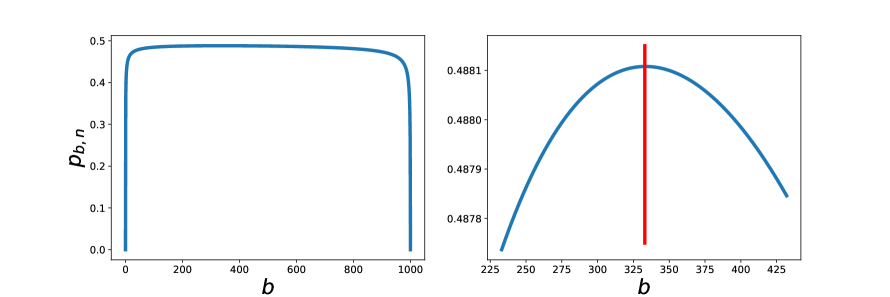
Figure 1: Plot of $p_{b,n}$ for $n=1000$, for all values of $b$ (left) and for $b\in[n/3-100,n/3+100]$ (right). Red line represents $n=3b+1$ – point of monotonicity change.

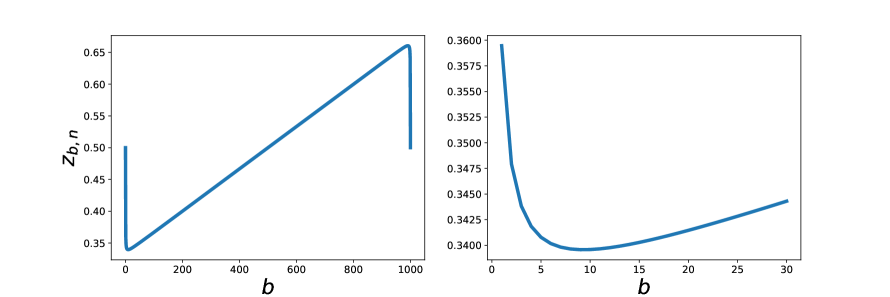
Figure 2: Plot of $z_{b,n}$ for $n=1000$, for all values of $b$ (left) and for $b\leq\sqrt{n}$ (right).

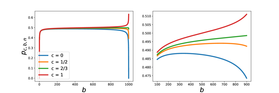
Figure 3: Plot of $p_{c,b,n}$ for $n=1000$, for $c\in\{0,\frac{1}{2},\frac{2}{3},1\}$ for $0\leq b\leq n$ (left) and for $\frac{n}{10}\leq b\leq\frac{9n}{10}$ (right).