Statistical Properties of ^56-57Fe with Multi-Shell Degrees of Freedom

Abstract

We investigate the statistical properties of ^56-57Fe within a model capable of treating all the nucleons as active in an infinite model space including pairing effects. Working within the canonical ensemble, our model is built on single-particle states, thus it includes shell and subshell closures. We include spin correlation parameters to account for nucleon spin multiplicities. Pairing and shell effects are important in the low temperature region where the quantum effects dominate. The validity of the model is extended to higher temperatures, approaching the classical regime, by including continuum states. We present results for excitation energy, heat capacity and level density of ^56-57Fe. The resulting favorable comparisons with experimental data and with other approaches, where applicable, indicate that the methods we develop are useful for statistical properties of medium to heavy nuclei.

year number number identifier Date text]date LABEL:FirstPage101 LABEL:LastPage#1102

I Introduction

Iron nuclei, especially ⁵⁶Fe, are the foci of extensive studies within various approachesAlhassid et al. (2015); Rombouts et al. (1998); Nakada and Alhassid (1998); Liu et al. (2000); Nakada and Alhassid (1997) since these nuclei play a major role in astrophysics Nakada and Alhassid (1997). The iron nuclei are the heaviest nuclei created by fusion of charged particles inside stars, and the starting point of the synthesis of heavier nuclei. Indeed, the statistical properties of ⁵⁶Fe are critical for our understanding of the fundamental nucleosynthesis processes in iron rich stars and cataclysmic astrophysical events such as neutron star mergers.

A major thrust of the present work is to develop a statistical method suitable for reaching higher temperatures by allowing the participation of all the nucleons. Another motivation for investigating ⁵⁶Fe is to compare our methods with another modern approach also available for this system. Furthermore, a comprehensive experimental list of states exists for ⁵⁶Fe Firestone and Baglin (1998) as well as experimental level densities for ^56,57Fe Schiller et al. (2003, 2000).

Theoretical results for how the excitation energy depends on temperature and how the level density changes with excitation energy for ⁵⁶Fe are available from Nakada and Alhassid Nakada and Alhassid (1997). Their results are obtained using the auxiliary field Monte Carlo shell model or “Shell Model Monte Carlo" (SMMC) method. Another version of the Monte Carlo shell model has also been used by Rombouts, Heyde, and Jachowicz (RHJ) Rombouts et al. (1998) to obtain ⁵⁶Fe statistical properties. Finally, a simple but useful phenomenological formula, the well-known Bethe formula, can be used to compare with various results for the level densities. The parameters of the back-shifted Bethe formula (BBF) for ⁵⁶Fe have been determined Shlomo and J.B.Natowitz (1990); Paar and Pezer (1997).

In this investigation, we utilize the single-particle (SP) spectra and, together with a phenomenological treatment of particle-particle correlations, to develop the properties of the multi-particle system using the canonical ensemble. The SP spectra can be simple, such as the three-dimensional harmonic oscillator, or more realistic, such as states obtained from a phenomenological SP potential Rombouts et al. (1998) or provided by Hartree-Fock (HF) Pratt (2000). The SP states are then thermally populated with an approximate treatment of interaction effects to produce the full system’s partition function. Observables, such as excitation energy, heat capacity, and level densities, can be directly computed. We call this method the “Statistical Mechanics using Single Particle States”(SMSPS).

Our approach models the situation of a specific set of nucleons, for example those that comprise the ⁵⁶Fe nucleus, embedded in a thermal bath such as the environment of a neutron star or a plasma produced during neutron star mergers. One of our goals is to simulate the physics of excitations that extend beyond those of the valence degrees of freedom alone. That is, we incorporate core excitations and excitations into the resonance and continuum regions. Given this span of thermal excitations, our approach must remain elementary in several aspects to make the calculations feasible.

In order to address the nuclear response over a very wide range of temperatures, we adopt a nuclear Hamiltonian that includes a mean field for all nucleons and a residual pairing interaction for nucleons occupying valence states. For states below the valence states we retain only the mean field Hamiltonian. Furthermore, we identify an approximate boundary in excitation energy between resonance states of the mean field and non-resonant continuum states. The resonant states are adopted from the quasi-bound states solutions of the mean field. The non-resonant states are taken to be the single-particle states of a spherical cavity that are smoothly joined by an average energy shift to the resonant state spectrum. The continuum state spectrum naturally depends on the volume (or radius of the spherical cavity) assigned to the nucleus in the thermal medium. In the case of the neutron star, this volume is controlled by external parameters such as gravity and rotation rate of the star.

The SMSPS model has two significant advantages: The first advantage arises, due to the neglect of inter-nucleon interactions, from the exact statistical population of these states which dramatically reduces the computation time. The second advantage is the ability to use a realistic SP spectrum as an input. For example, the SP states will reflect the long-range Coulomb repulsion in the proton degrees of freedom by incorporating the repulsive shift in the proton states relative to the neutron states. This distinct SP spectra, one for protons and one for neutrons, is a dominant aspect of charge dependence in medium and heavy nuclei.

In this investigation, the SP states provided by Ref.Rombouts et al. (1998) are employed within the SMSPS. In section (II) we introduce our approach to the canonical ensemble and present its results. In Section (III) we present an inter-comparison of our results with experimental data and with the Bethe formula. Section (IV) presents our conclusions and outlook to the future.

II Statistical Spectroscopy of The Nuclear System

II.1 The Single Particle Partition Function

The first basic ingredient of our model is the Hamiltonian which can be written as

$$\hat{H}=\hat{H}_{m}+\hat{H}_{P},$$ (1)

where $H_{m}$ is the mean field Hamiltonian, and $H_{P}$ is a Hamiltonian that accounts for the residual or "effective" interactions that induce correlations beyond those accommodated by the mean field. For open-shell nuclear systems, such as ⁵⁶Fe, the nuclear pairing Hamiltonian Chasman (2003) is particularly important. For our specific application, we therefore include pairing interaction contributions to states above the Fermi level. The second ingredient of our approach is the SP partition function $\mathcal{Z}_{1}$ defined as

$$\mathcal{Z}_{1}(\beta) = \underset{\mathcal{Z}_{1}^{\text{SPS}}}{\underbrace{\sum_{\alpha,k}\left\langle\psi_{\alpha}^{(k)}\left|e^{-\beta\hat{H}}\right|\psi_{\alpha}^{(k)}\right\rangle}}+$$ (2)

$$\underset{\mathcal{Z}_{1}^{\text{cont}}}{\underbrace{\frac{4\pi V}{h^{3}}\int_{\sqrt{2mE_{\max}}}^{\infty}e^{-\beta\frac{p^{2}}{2m}}p^{2}dp}}.$$

Here, the index $\alpha$ denotes the set of quantum numbers of each, possibly degenerate, state and $k$ labels the degenerate substates. $E_{\max}$ denotes an energy cutoff defining the maximum resonance state of the mean field Hamiltonian, $V$ denotes the volume of continuum state. The first term in the RHS of Eq.(2) represents the sum of the discrete single-particle states (SPS) generated by the mean field Hamiltonian plus the effect of the residual interaction. The 2^nd term in the RHS of Eq.(2) represents the sum of continuum states and the integral can be computed to yield

$$\mathcal{Z}_{1}^{\text{cont}}(\beta,V) = V\left(\frac{2\pi m}{h^{2}\beta}\right)^{3/2}\times$$ (5)

$$\left(\begin{array}[]{c}1+2\sqrt{\frac{\beta E_{\max}}{\pi}}e^{-\beta E_{\max}}-\\ \mathrm{erf}\left(\sqrt{\beta E_{\max}}\right)\end{array}\right).$$

Assuming the adopted mean field has spherical symmetry (which we adopt here) there is degeneracy with respect to angular momentum projection, $m_{J_{\alpha}}$, the sum over discrete states can be written as

$$\mathcal{Z}_{1}^{\text{SPS}}(\beta) = \sum_{\alpha}g_{\alpha}e^{-\beta\left(\varepsilon_{\alpha}+\langle\hat{H}_{P}\rangle\right)},$$ (6)

$$= \sum_{\alpha}\sum_{m_{J_{\alpha}}=-J_{\alpha}}^{+J_{\alpha}}e^{-\beta\left(\varepsilon_{\alpha}+\langle\hat{H}_{P}\rangle\right)},$$

where $g_{\alpha}=\sum_{k}\left\langle\psi_{\alpha}^{(k)}|\psi_{\alpha}^{(k)}\right\rangle$ is the degeneracy for the $\alpha^{\text{th}}$ state. The partition function in Eq.(6) represents the partition function of SPS plus pairing. One common description that links pairing correlations to thermal effects is implemented within the Bardeen-Cooper-Schrieffer theory. In BCS the pairing Hamiltonian is expressed by

$$\hat{H}_{P}=G\sum_{\alpha}a^{\dagger}_{\alpha}a^{\dagger}_{\bar{\alpha}}a_{\alpha}a_{\bar{\alpha}},$$

where $\alpha$ and $\bar{\alpha}$ denote a state and its time-reversed state, respectively. To have this model effective for hot nuclei, a thermal population of particles among the states is used, mainly by implementing a Monte-Carlo technique Alhassid et al. (2015); Rombouts et al. (1998); Nakada and Alhassid (1998); Alhassid et al. (2016). This technique, however, requires significant computational resources, even for limited orbits in the proximity of the valence shell. Another model for including pairing effects is based on Hartree-Fock-Bogoliubov (HFB) Martin et al. (2003); Khan et al. (2007) theory. However, the HFB model is limited by particle number fluctuation and quasi-particle parity mixing issues Gambacurta et al. (2013, 2014). In our approach, as commonly done in BCS calculations at zero temperature, the pairing interaction is considered acting only on energy levels above the Fermi level. Phenomenologically we can express this effect on the energy levels as

$$\langle\hat{H}_{P}\rangle=\theta(\varepsilon_{f})\Delta(\beta),$$ (7)

where $\theta(\varepsilon_{f})$ is the step function

$$\theta(\varepsilon_{f})=\begin{cases}1;&\text{if }\varepsilon_{\alpha}>\varepsilon_{f},\\ 0;&\text{if }\varepsilon_{\alpha}\leq\varepsilon_{f}.\end{cases}$$

Thus the SP partition function in Eq.(6) becomes

$$\mathcal{Z}_{1}^{\text{SPS}}(\beta)=\sum_{\alpha}g_{\alpha}\,e^{-\left[\varepsilon_{\alpha}+\theta(\varepsilon_{f})\Delta(\beta)\right]\beta}.$$ (8)

The effect of the pairing is to increase the energy gap of the Fermi level. The gap shift $\Delta$ is set to be temperature dependent, expected to be maximum near zero temperature and to decrease as temperature increases to reach zero at a higher temperature. The calculation of $\Delta$ will be discussed in sec.III.

Within the framework of the SMSPS the effects of pairing and spin-orbit splitting are averaged by arranging the nucleons using a technique, which we call configuration-restricted recursion. We implement this technique for a fixed species of protons or neutrons by constructing the partition function for a subgroup of that species that, for example, limits the values of the magnetic projection of the total angular momentum quantum number to positive values, signified by $|m_{J}|$. Thus, we obtain the SPS partition function of that restricted range, denoted as $\left(\mathcal{Z}_{1}^{\text{SPS}}\right)^{\left|m_{J}\right|}$, and given by

$$\left[\mathcal{Z}_{1}^{\text{SPS}}(\beta)\right]^{\left|m_{J}\right|}=\sum_{\alpha}\sum_{m_{J_{\alpha}}=J_{\alpha},J_{\alpha}-1,\ldots>0}\exp\left(-\beta E_{\alpha}\right),$$ (9)

where $E_{\alpha}=\varepsilon_{\alpha}+\theta(\varepsilon_{f})\Delta(\beta)$. With symbol “$-\left|m_{J}\right|$”, we signify that magnetic state summation in the partition function $\left(\mathcal{Z}_{1}^{\text{SPS}}\right)^{-\left|m_{J}\right|}$ runs over negative values $\left(-J_{\alpha},-J_{\alpha}+1,\ldots<0\right)$. Making use of Eq.(5) and Eq.(9) within Eq.(2) we obtain $\mathcal{Z}_{1}^{\left|m_{J}\right|}$

$$\mathcal{Z}_{1}^{\left|m_{J}\right|}(\beta)=\left[\mathcal{Z}_{1}^{\text{SPS}}(\beta)\right]^{\left|m_{J}\right|}+\mathcal{Z}_{1}^{\text{cont}}(\beta,V).$$ (10)

II.2 The Nuclear Partition function and Observable Calculations

We then recur the partition function in Eq.(10) for the given $m$-projected configurations of $Z_{1}$ protons (or $N_{1}$ neutrons) using the recursion formula for spinless identical fermions, given in Ref.Borrmann and Franke (1993). This formula for $n$ identical spinless (or polarized) fermions is

$$\mathcal{Z}_{n}(\beta)=\frac{1}{n}\sum_{\nu=1}^{n}(-1)^{\nu+1}\mathcal{Z}_{1}(\nu\beta)\mathcal{Z}_{n-\nu}(\beta),\qquad\mathcal{Z}_{0}(\beta)=1,$$ (11)

where $n$ has to be replaced by $Z_{1}$ for the proton case ($N_{1}$ for the neutron case) in the $|m_{J}|$ states and by $Z_{2}$ for the proton case ($N_{2}$ for the neutron case) in the $-|m_{J}|$ states. We denote $Z=Z_{1}+Z_{2}$ as the total number of protons, $N=N_{1}+N_{2}$ as the total number of neutrons, and $A=Z+N$ as the total number of nucleons. Note that for even $Z$ (or $N$) then $Z_{1}=Z_{2}=Z/2$ (or $N_{1}=N_{2}=N/2$). For odd $Z$ (or $N$) we choose $Z_{1}=(Z+1)/2$ and $Z_{2}=(Z-1)/2$ (or $N_{1}=(N+1)/2$ and $N_{2}=(N-1)/2$).

The recursion formula (11) gives exact values of the partition functions at specific values of $n$ and $\beta$. Up to this point we obtain $\mathcal{Z}_{Z_{1}}^{\left|m_{J}\right|}$ and $\mathcal{Z}_{N_{1}}^{\left|m_{J}\right|}$ for $Z_{1}$ protons and $N_{1}$ neutrons, respectively, which thermally populate the $|m_{J}|$’s states. Following the corresponding procedure, we now obtain $\mathcal{Z}_{Z_{2}}^{-\left|m_{J}\right|}$ and $\mathcal{Z}_{N_{2}}^{-\left|m_{J}\right|}$ for $Z_{2}$ protons and $N_{2}$ neutrons that populate the $-|m_{J}|$’s states.

The total nuclear partition function is constructed by

$$\mathcal{Z}_{A}(\beta)=\left(\mathcal{Z}_{Z_{1}}^{\left|m_{J}\right|}\mathcal{Z}_{Z_{2}}^{-\left|m_{J}\right|}\right)\left(\mathcal{Z}_{N_{1}}^{\left|m_{J}\right|}\mathcal{Z}_{N_{2}}^{-\left|m_{J}\right|}\right),$$ (12)

With this product in Eq.(12) of restricted sub-configuration partition functions, the total magnetic projection quantum number is restricted, on average, to zero for each nucleon species (protons or neutrons). Thus, the fact that each nucleon species occupies SP states predominantly in spin-paired configurations is taken into account, on average.

Eq.(12) also implies that, at sufficiently high $\beta$, due to the degeneracy of time-reversed single particle states, for each proton (or neutron) in state $\left|J_{\alpha}^{(Z_{1})},|m_{J_{\alpha}}^{Z_{1}}|\right\rangle$ (or $\left|J_{\alpha}^{(N_{1})},|m_{J_{\alpha}}^{N_{1}}|\right\rangle$), there exists another proton (or neutron) in state $\left|J_{\alpha}^{(Z_{2})},-|m_{J_{\alpha}}^{Z_{2}}|\right\rangle$ (or $\left|J_{\alpha}^{(N_{2})},-|m_{J_{\alpha}}^{N_{2}}|\right\rangle$) with the same statistical weight. Then, as $\beta$ decreases, excitations enter that break this symmetry while retaining only a total $M=0$ constraint for each nucleon species. We believe that this feature of our total partition function is reasonable since we expect that polarization effects are minimal at zero temperature and those polarization effects beyond simple thermal excursions that are accommodated here are unlikely to contribute as temperature increases.

In this way, we approximate average pairing of total spin projections suitable for the low to moderate excitation region. The additional coherent pairing energy associated with the ground state and lowest-lying states is very important when we calculate the level density for an open-shell even-even nucleus. This will be addressed phenomenologically when calculating level densities via the parameter $\Delta$ in Eq.(7). The configuration-restricted recursion technique and the coherent pairing energy shift defines our proton-proton and neutron-neutron correlation approach in our SMSPS theory.

Once the nuclear partition function is computed for the desired system at a given temperature, the observables such as the average thermal energy $E_{A}$, the heat capacity $C_{A}$, and the number of levels per unit energy $g_{A}$ can be computed, respectively, in the canonical ensemble as Fowler et al. (1978)

$$E_{A}(\beta)=-\frac{\partial}{\partial\beta}\log Z_{A}(\beta);\quad C_{A}(\beta)=-k_{B}\beta^{2}\frac{\partial E_{A}}{\partial\beta},$$ (13)

and

$$g_{A}(E) = \frac{\beta e^{S(\beta)/k_{B}}}{\sqrt{2\pi C_{A}(\beta)/k_{B}}},$$ (14)

$$= \frac{\beta}{\sqrt{2\pi C_{A}(\beta)/k_{B}}}Z_{A}(\beta)e^{\beta E_{A}(\beta)}.$$

The factor $Z_{A}(\beta)\exp\left(\beta E_{A}(\beta)\right)$ is the number of microstates $\Omega_{A}(E)$. We also notice that the heat capacity and the level densities are independent of the lowest-state energy $E_{\mathrm{gs}}$ as expected. We can easily prove in the canonical ensemble that Shehadeh (2003)

$$\Delta E\equiv\sqrt{\left\langle E_{A}^{2}\right\rangle-\left\langle E_{A}\right\rangle^{2}}=\frac{1}{\beta}\sqrt{C_{A}(\beta)/k_{B}}.$$ (15)

Therefore Eq.(14) can be written as

$$g_{A}(E)=\frac{1}{\sqrt{2\pi}}\frac{\Omega(E)}{\Delta E}.$$

As $\beta\rightarrow\infty$, $\Delta E\rightarrow 0$ and the statistics become very low. Thus, at $T=0$ we switch over to the micro-canonical ensemble to obtain level densities Shehadeh (2003).

III Results and Discussion

Our investigation falls into two main categories: First the effect of model space on observable quantities such as excitation energy $E_{x}$, heat capacity $C$, and level density $\rho$ of ^56,57Fe. Second, the effect of pairing on SP states and how incorporating this effect would improve level densities $\rho$ versus experimental results. In both categories, We use SPS of the mean field spectrum of the Woods-Saxon (WS) potential with phenomenological parameters as described in Ref.Rombouts et al. (1998) to evaluate the thermal properties of ^56,57Fe. The SPS energy levels and model space divisions are shown in Fig(1).

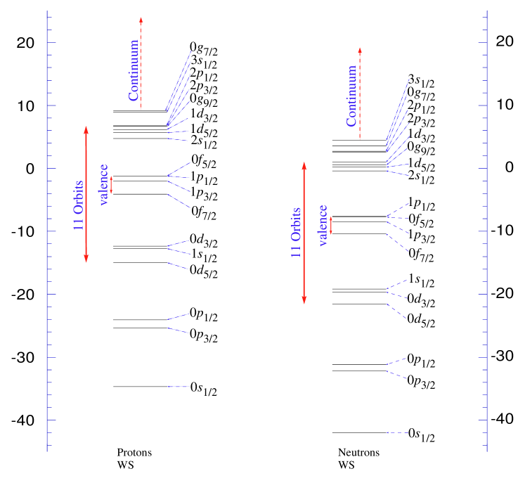
Figure 1: (Color online) The single-particle (SP) energy levels in MeV of ^56,57Fe from Wood-Saxon (WS) calculations of Ref.Rombouts et al. (1998) indicated as horizontal bars. For the proton levels, the Coulomb potential of a uniformly charged sphere is included. Vertical arrows indicate the level groupings used in the calculations. The continuum region is added smoothly to the discrete spectra as discussed in the text.

To be able to reach the lowest possible temperature for larger model spaces we implement a multi-precision algorithm called “quad double" developed by Hida and Bailey Hida et al. (2001, 2000) which enables us to compute observables up to 212 bits of floating-point accuracy. At very low temperature and large model space, we implement ARbitrary PRECision Computation Package (ARPREC) Bailey et al. (2018) which enables us to compute at 200 digits after the decimal point. We are able to obtain stable results for the canonical ensemble down to $T=1.37$ MeV for our no-core model space.

III.1 The Model Space Effect

In this subsection (covering results presented in Figs.2-6), we set our pairing shift parameter $\Delta=0$. We carry out the computations for three divisions of the model spaces, shown in Fig.(1). These three choices allow us to investigate the model space dependence of results over a range of temperatures. Starting from a simple valence 4 orbits $0f_{7/2}1p_{3/2}1p_{1/2}0f_{5/2}$ which contains 6 protons and 10 neutrons for ⁵⁶Fe (11 neutrons for ⁵⁷Fe) leaving an inactive core of 20 protons and 20 neutrons. We simply refer to this model space as 4 orbits. The second model space consists of 18 protons and 22 neutrons for ⁵⁶Fe (23 neutrons for ⁵⁷Fe) in 11 orbits, and runs from the $0d_{5/2}$ state to the$0g_{9/2}$ state, leaving a core of 8 protons and 8 neutrons. We refer to this model space as 11 orbits. The final model space is the no-core case which includes all available orbits (18 orbits) and continuum to attain a no core system. The volume of the continuum state is considered to be a spherical cavity with a radius equal to 2.3 times the mean nuclear radius. We adopt a mean nuclear radius $R=r_{0}A^{1/3}$ where $r_{0}=1.25$ fm. Thus $R=4.78$ fm for ⁵⁶Fe and $R=4.81$ fm for ⁵⁷Fe. Support for this choice of volume for the continuum states will be presented when we discuss the heat capacity.

Fig.(2) shows the excitation energy of ^56,57Fe versus temperature computed with SMSPS using 4-orbit, 11-orbit, and no-core model spaces. Here, the excitation energies of the SMSPS are compared with the excitation energy obtained for ⁵⁶Fe using the Shell-Model Monte Carlo (SMMC) method of Nakada and Alhassid Nakada and Alhassid (1997). The SMMC is a standard technique since it includes a microscopic Hamiltonian that accounts for important residual interactions.

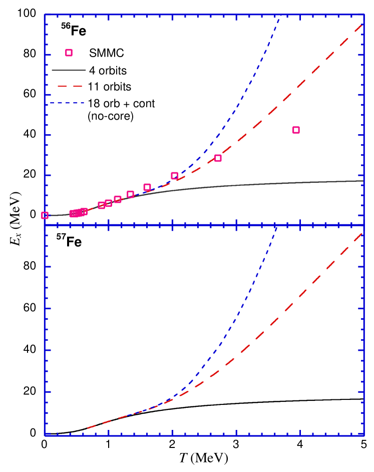
Figure 2: (Color online) The SMSPS excitation energies (in MeV) versus temperature (in MeV) with pairing set to zero for ⁵⁶Fe (top) and ⁵⁷Fe (bottom) computed at various model spaces, 4 orbits, 11 orbits and 18 orbits+cont (the no-core case) (see common legend). The results for ⁵⁶Fe are compared with those of the SMMC in Ref.Nakada and Alhassid (1997).

The general trend for the excitation energy is that it is zero at and near zero temperature and it does not exhibit any significant increase for $T<0.2$ MeV. This indicates the thermal energy is insufficient to excite nucleons to higher valence states. As temperature increases above $T=0.2$ MeV, internal energy increases rapidly with temperature. The rate of rising excitation energy with temperature tapers off for 4 orbits and then for 11 orbits model spaces, as the model space eventually cuts off and yields no additional higher-energy states for the excited nucleons to occupy. That is, the internal energy saturates towards the maximum energy offered by the quantum configurations of these limited model spaces. Thus, above a certain temperature a larger model space is needed to provide more particles and states to contribute to the excitation energy.

The SMSPS 4 orbits results agree well with those of the SMMC up to $T\leq 1$ MeV. The results of the SMSPS for $T\leq 1$ MeV are controlled by phenomenological SP spectra that are in good agreement with experimental information. Beyond the 1 MeV temperature, the SMSPS results lie below those of SMMC even for higher model spaces. Note that the SMMC results are obtained with an additional orbital, the $0g_{9/2}$, included within its valence space. We observe that when we include this orbital and additional orbitals in the 11 orbit space, we extend the temperature range over which our SMSPS results agree with the SMMC results. We also observe that the SMSPS internal energy is close to the internal energy predicted in Ref.Rombouts et al. (1998) using the shell-model quantum Monte Carlo method and pairing strength $G=20$ MeV/56 which we attribute to our use of the same SP spectra.

To expand the range of applicability of the SMSPS, especially for $T\geq 1$ MeV, we increase the model space to 18 orbits with the continuum (no-core). For the no-core model space we are able to extract reliable results when $T\geq 1.5$ MeV by implementing high precision algorithms of Refs.Hida et al. (2001, 2000); Bailey et al. (2018) within the SMSPS code. Going lower in temperature with no core model space is possible with increasing number of significant digits of the code’s variables. The computation time, however, becomes lengthy. Thus we truncate the minimum temperature limit for larger model spaces such that the results of larger model spaces join smoothly with the results in the smaller model spaces.

In the case of ⁵⁷Fe, there are 11 neutrons in the $fp$ shell at T = 0. Therefore, this isotope has a leading unperturbed configuration which is one neutron less than needed to fill the $1p_{3/2}$ subshell. We found that the addition of one neutron to ⁵⁶Fe does not have a significant contribution to the excitation energy as a function of $T$ as seen by comparing results in the two panels of Fig.(2). Although it is not apparent from Fig.(2), for $E_{x}\geq 1$ MeV in the 4 orbit model space the ⁵⁶Fe excitation energy as a function of $T$ is slightly greater than that of ⁵⁷Fe. This apparent paradox arises from the fact that, in this limited model space the ratio of the number of accessible states for excitation to the number of nucleons is sufficiently smaller for ⁵⁷Fe. Therefore, there are fewer degrees of freedom for excitation for the neutrons for $E\geq 1$ MeV in ⁵⁷Fe and it is closer to saturating the 4 orbit model space than is ⁵⁶Fe.

Fig.(3) displays the SMSPS heat capacity for ^56,57Fe as a function of temperature for the three model spaces, 4 orbits, 11 orbits, and no-core as described in Fig.(1). For the 4-orbit model space, the maximum heat capacity occurs when one starts exciting nucleons from the inner valence state (the $0f_{7/2}$ state). The neutron heat capacity at the peak is somewhat larger than the proton’s reflecting the larger number of neutron degrees of freedom in this model space.

Because there is a small energy spacing between the $1p_{3/2}$ and the $0f_{5/2}$ single-neutron states (0.78 MeV) the neutron heat capacity is larger than the proton’s in the low temperature region for both ⁵⁶Fe and ⁵⁷Fe. In fact, there is a small hump in the total heat capacity which comes entirely from the neutron heat capacity at $T=0.2$ MeV, barely visible in Fig.(3) for ⁵⁶Fe but more apparent for ⁵⁷Fe. This signifies the excitation from the $1p_{3/2}$ state to the $0f_{5/2}$ and $1p_{1/2}$ states since they are nearly degenerate. By contrast, the lowest proton excitation is more than 2 MeV from the $0f_{7/2}$ to the $1p_{3/2}$ state. The SMSPS heat capacity for ⁵⁷Fe, where we have 3 neutrons in the $1p_{3/2}$ instead of 2 neutrons in the ⁵⁶Fe case, shows an enhanced hump at $T=0.2$ MeV.

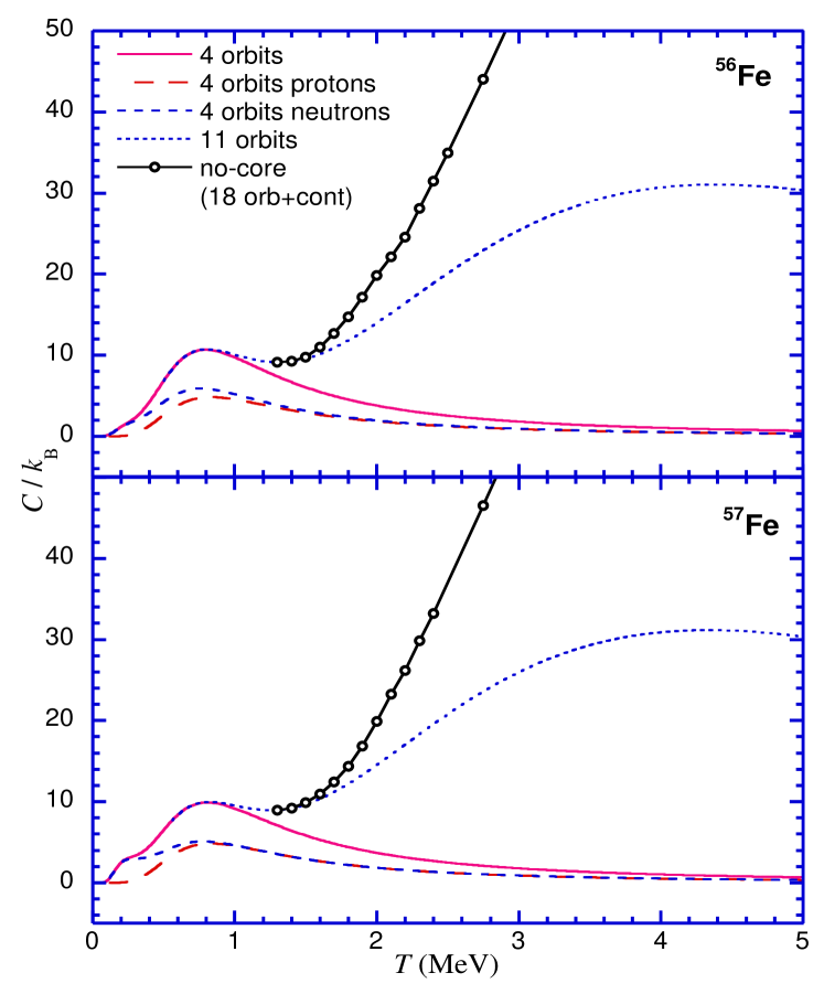
Figure 3: (Color online) The SMSPS Heat capacity versus temperature (in MeV) with pairing set to zero for ^56,57Fe for three model spaces 4 orbits, 11 orbits, and 18 orbits+cont (no-core). The legend is common for the top and bottom figures.

Both ^56,57Fe heat capacities exhibit a prominent peak in heat capacity near $T=0.8$ MeV. The expanding model spaces, exhibited for ^56,57Fe, show that this feature survives as the core degrees of freedom are brought into the calculation. We therefore identify this major heat capacity peak as an indicator of what we call “Total Valence Melting”(TVM) since it signifies thermally exciting all the valence nucleons from their $T=0$ subshells.

The core contribution to heat capacity above the TVM temperature is very important. Any consideration of the heat capacity beyond TVM temperature must include the inner-shell nucleons and higher lying orbits. Below the TVM temperature, however, all model spaces produce exactly the same behavior. This is understandable since at sufficiently low temperatures the valence nucleons dominate. We conclude that valence shell contributions to the excitation energy and heat capacity are dominant for $T<1.0$ MeV.

Fig.(4) shows the SMSPS heat capacity for ^56,57Fe computed at no core model space including the continuum for an extended temperature range. There is another maximum for heat capacities at $T=8.8$ MeV, which marks the transition from resonance states to the continuum. The value and the position of this maximum depend on the continuum state volume: the larger the volume - the larger the maximum. As we vary the volume, the position of the maximum versus temperature can shift either towards higher temperature or towards lower temperature. We fix the volume such that the maximum is located at a temperature corresponding to the binding energy per nucleon. In case of ^56,57Fe $BE/A\approx 8.8$ MeV we find there is a unique value for the spherical volume of the continuum which satisfies this condition - when the radius of the volume equals to 2.3 mean nuclear radius of ^56,57Fe.

The rise of the value of the maximum when the volume increases, implies that the system finds it more favorable, as expected, to excite nucleons from resonance states to continuum states. We note that this maximum corresponds to the beginning of a phase transition from quantum gas to classical gas regime since the values of the heat capacities $C/k_{B}$ are trending towards the classical value $\frac{3}{2}A$ ($84$ for ⁵⁶Fe and 85.5 for ⁵⁷Fe).

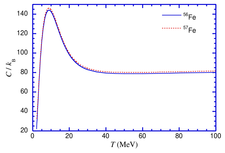
Figure 4: (Color online) The SMSPS heat capacities versus temperature (in MeV) with pairing set to zero for ^56,57Fe in 18 orbits+cont (no-core) model space. The continuum is computed for a sphere with radius equal to 2.3 times the root mean square nuclear radius.

Fig.(5) displays the level densities at low excitation energies of ^56,57Fe predicted by the SMSPS and compared with results from other methods and with experiment where available. The SMSPS is computed for valence shells only. As we can understand from $E_{x}$ vs $T$ and $C$ vs $T$ graphs the valence contribution is sufficient for $T<1.0$ MeV or $E_{x}<6.0$ MeV. The experimental level density is histogrammed into 1 MeV bins using the state list in Ref.Firestone and Baglin (1998). The experimental spectrum appears incomplete for $E_{x}>4.0$ MeV. The circular points in the figure represent the experimental level densities extracted from primary $\gamma$ spectra for ^56,57Fe nuclei obtained with (³He, $\alpha\gamma$) and (³He, ³He$\gamma$) reactions on ^56,57Fe targets using the Oslo method (OM) Schiller et al. (2003, 2000).

The Bethe backshifted formula values (BBF) displayed in Fig.(5) are computed using Shlomo and J.B.Natowitz (1990); Paar and Pezer (1997)

$$g(E_{x})=g_{0}\frac{\sqrt{\pi}}{24\sigma}a^{-\frac{1}{4}}\left(E_{x}-\delta\right)^{-\frac{5}{4}}\exp\left(2\sqrt{a\left(E_{x}-\delta\right)}\right),$$ (16)

where $g_{0}=\sqrt{2/\pi}$ and $\sigma$ is the spin cut-off parameter given by Gilbert and Cameron (1965)

$$\sigma^{2}=0.0888A^{2/3}\sqrt{a\left(E_{x}-\delta\right)}.$$ (17)

For ⁵⁶Fe, we choose the backshift parameter $\delta=1.38$ MeV Woosley et al. (1978) and the value $a=A/K$ Natowitz et al. (2002) where $K=7$ MeV. The same parameter values are employed for ⁵⁷Fe, except for the backshift parameter $\delta=0$ MeV. This yields a level density that agrees very well with the experimental state counts and OM level density points for $E_{x}<4.0$ MeV. At higher excitation energies, we expect the theory to be higher than the experiment as the reaction mechanism becomes less successful in reaching states of higher angular momentum.

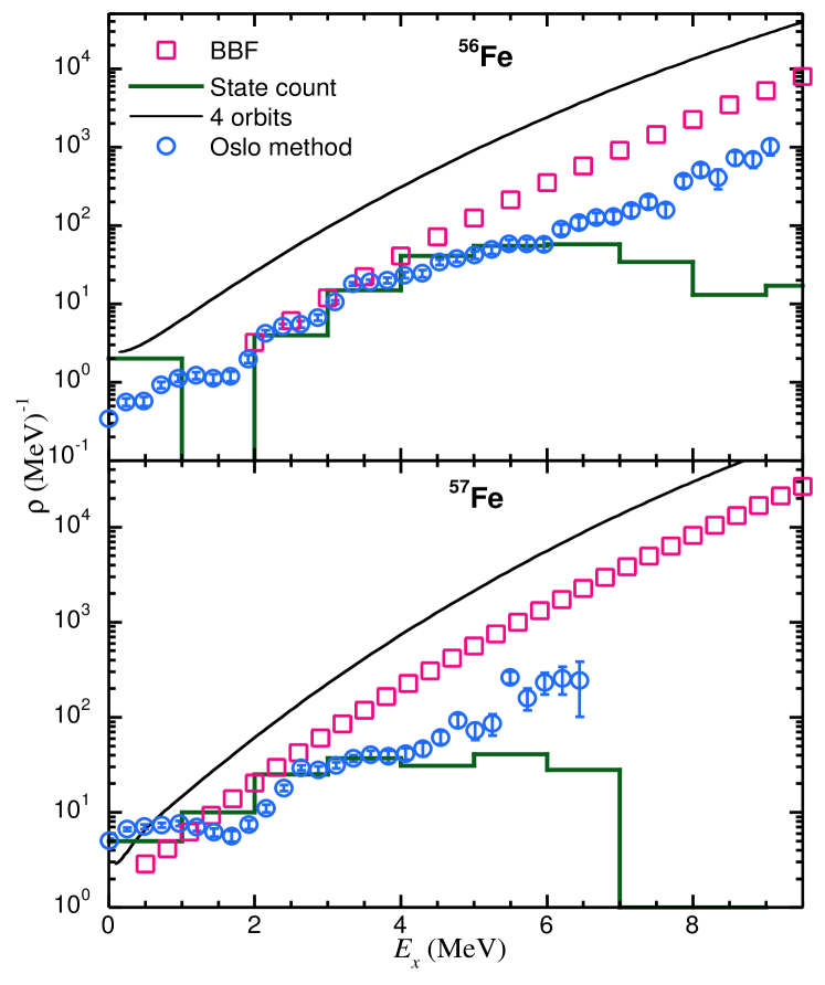
Figure 5: (Color online) The SMSPS level density of ^56,57Fe with pairing set to zero computed using 4 orbits (valence shell) is compared with various results. The histogram is the experiment. The BBF level density is evaluated using Eq.(16) with backshift parameter $\delta=1.38$ MeV Woosley et al. (1978) and $a=8$ MeV^-1 for ⁵⁶Fe, and $\delta=0$ MeV and $a=8.143$ MeV^-1 for ⁵⁷Fe. The top and bottom figures have common legend.

Without pairing, the SMSPS results for ⁵⁶Fe overestimate level density, almost systematically. If the same backshift parameter used in the BBF ($\delta=1.38$ MeV) is applied to the SMSPS model, the resulting curve would describe well the experimental results at low excitations. This backshift value is an approximate correction to estimate the coherent pairing energy shift which we expect will arise when we include our treatment of pairing in the next subsection.

A similar behavior of SMSPS level density without pairing is obtained for ⁵⁷Fe but with a somewhat better agreement with BBF and experiment. The addition of the odd neutron in the valence shell lowers the deficit from the missing pairing contributions which in turns improves the agreement between SMSPS values (absent pairing) with experiment and BBF’s. We also notice in Fig.(5) the level density of ⁵⁷Fe is higher than that of ⁵⁶Fe since the extra neutron is unpaired and can be excited easily to higher states. For $E_{x}>15.5$ MeV SMSPS level densities at any model space, as shown in Fig.(6), lie lower than the BBF values. Thus, the SMSPS density of states suggest a slower exponential increase with excitation energy than that obtained with the BBF using conventional parameter selections.

To investigate the model space dependence of the level density prior to including pairing effects, we calculate the SMSPS level density for ^56,57Fe at 11 orbits and 18 orbits+continuum (no-core) as shown in Fig.(6). Model space limits inhibit the rate of increase in the level density. In fact, every finite model space produces a curve that reaches some saturated value as seen with the 4 orbit level density in Fig.(6). In the figure all level density curves for different model spaces coincide for $E_{x}<15$ MeV where the 4-orbit model space (valence orbits only) is adequate to describe the system’s level density. Above 15 MeV it appears safer to adopt a larger model space of at least 11 orbits. For $E_{x}>20$ MeV we need a no-core model space to describe the level density. Above 21 MeV the effect of the continuum is imperative and has to be incorporated into the calculation for reliable results.

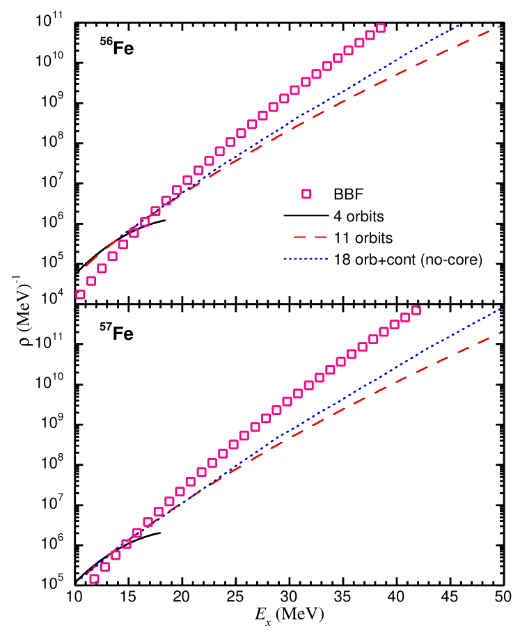
Figure 6: (Color online) The level densities with pairing set to zero for ^56,57Fe calculated at higher excitations at larger model spaces see legend.

III.2 The Pairing Effect

We have commented that shifting the excitation energies by 1.38 MeV (the same energy shift used in BBF) improves SMSPS level density for ⁵⁶Fe towards reproducing the experimental and BBF values. Until now, we have not incorporated our treatment of pairing. Hence, we now adjust the energy gap of Fermi levels to obtain the shifted energy $E_{x}+1.38$ MeV at the same temperature $T$ that originally gives $E_{x}$. We perform this energy shift to cover all excitation energies and obtain sufficient data for $\Delta$ vs $T$. Fig.(7) shows the resulting pairing gap energy $\Delta$ as a function of temperature for ⁵⁶Fe and ⁵⁷Fe.

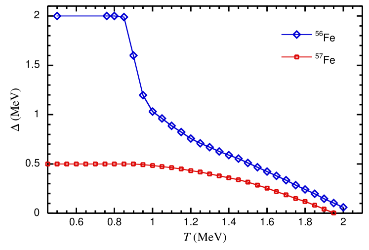
Figure 7: (Color online) the pairing energy gap $\Delta$ as a function of temperature $T$ for ⁵⁶Fe and ⁵⁷Fe.

For ⁵⁶Fe, when $T\leq 0.885$ MeV the value of $\Delta=2.01$ MeV is constant. Just when $T>0.885$ MeV, the value of $\Delta$ drops very rapidly until $T=1$ MeV. For $T>1$ MeV, $\Delta$ starts decreasing slowly with increasing $T$. In order to capture the correct $T$ at which $\Delta$ disappears, we computed the SMSPS for 11 orbits (18 protons and 22 neutrons) leaving only 8 protons and 8 neutrons as the inert core. The value of $\Delta$ diminishes at $T=2.065$ MeV. A much smoother behavior is noticed for ⁵⁷Fe. when $T\leq 0.906$ MeV, the value of $\Delta=0.501$ MeV is constant. When $T>0.906$ MeV $\Delta$ decreases smoothly as $T$ increases. This is an indication that the thermally active nucleons of ^56,57Fe are in a superfluid phase below these critical temperatures. This is similar to what Ref.Gambacurta et al. (2013, 2014) has concluded for ^161,162Dy and ^171,172Yb isotopes. The generated values of $\Delta$ are fitted as a function of $1/T$ using a 5th-degree polynomial and the fitting coefficients are fed into the SMSPS code to re-evaluate the partition functions and all of the observables at given temperature and energy gap $\Delta$.

Fig.(8) compares the heat capacities of the SMSPS and the SMSPS with $\Delta=0$. Both heat capacities are computed using 11 orbits. In both isotopes the TVM peaks of SMSPS with pairing are shifted towards higher $T$, and the humps disappear. This is expected since increasing the energy gap due to pairing prevents neutrons in the Fermi level from melting at low $T$. The hump must have been shifted to higher $T$ and disappeared under the TVM peak. The pairing effect increases the values of heat capacities since a higher temperature is needed to overcome the correlation among valence nucleons.

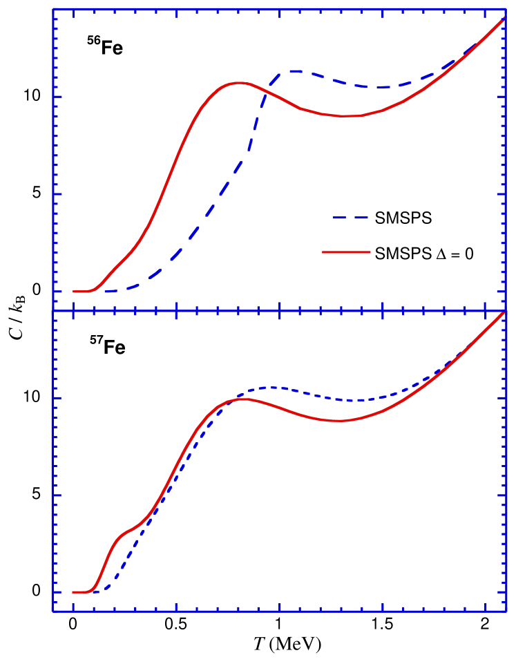
Figure 8: (Color online) The effect of the pairing on SMSPS heat capacities versus temperature (in MeV) for ⁵⁶Fe (top) and ⁵⁷Fe (bottom). All SMSPS results are computed at 11-orbit model space.

Fig.(9) shows the improvement that pairing brings to the SMSPS level densities for both ^56,57Fe. The agreement of the SMSPS with experimental data and BBF is gratifying. This agreement with BBF for ^56,57Fe extends to higher excitation energies, as Fig.(10) shows, beyond energies we used to evaluate $\Delta$ as a function of $T$.

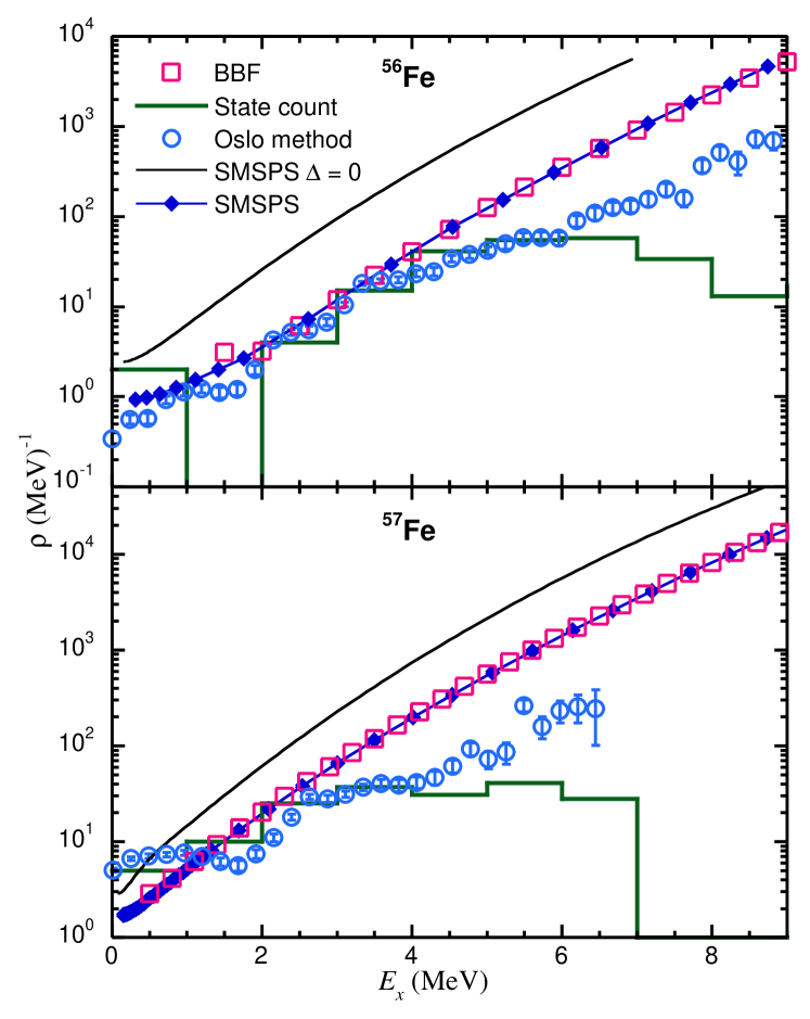
Figure 9: (Color online) Same as Fig.(5) but with paring included in the SMSPS level density of ^56,57Fe. The SMSPS is computed at 4-orbit model space. The top and bottom figures have a common legend.

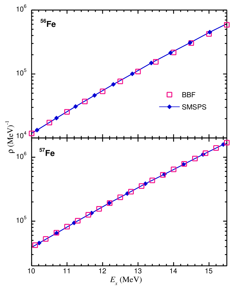
Figure 10: (Color online) Same as Fig.(6) with pairing included within the SMSPS high excitation level densities for ^56,57Fe compared with the BBF. The SMSPS is computed with the 11-orbit model space.

IV Conclusions and Outlook

We have shown that the SMSPS is a flexible tool to compute the thermal properties of isotopes in the Iron region. The SMSPS has the ability to produce results in both near zero and high temperature at large model spaces. Two primary variables needed to be adjusted in order to refine the SMSPS approach: (1) The volume of the continuum states which needs to be chosen such that the heat capacity exhibits a phase transition between quantum to classical gas at temperatures approximating the binding energy per nucleon, (2) The pairing parameter $\Delta$ which has to be calculated to achieve the correct backshift energy of the level density. The volume variable is crucial in the high-temperature region, whereas the pairing variable is important for even-even open-shell nuclei in the low temperature region. According to the SMSPS approach, $A=56$ and $57$ Iron isotopes have the following properties

1. For $0<T<0.9$ MeV these nuclei behave like a superfluid with significant pairing effects.

2. For $0.9<T<8.8$ MeV these nuclei exhibit properties reflective of a mixture of fluid (in the core) and quantum gas (in the valence and resonance states).

3. For $T>8.8$ MeV these nuclei exhibit the transition to a non-interacting classical gas.

The main advantages of the SMSPS are:

1. Depends on the chosen SP states which means that the SMSPS accommodates physically realistic shell structures, including shell closure effects.

2. The theory is capable of treating all nucleons as active in a model space that extends to continuum.

3. The theory can admit pairing correlations in a phenomenological manner.

4. The SMSPS theory is computationally inexpensive.

The disadvantages of the SMSPS are its sensitivity to the mean field SP states, and its lack of a microscopic Hamiltonian. However, if the energy gap function due to the paring correlation of such SPS is obtained and the volume parameter of the continuum state is determined, the SMSPS is found to yield excellent values of level densities. In the future, we will investigate alternative models for the SPS such as those from mean field theory. The SMSPS model may be further improved by refining the configuration-restricted recursion technique with input from a fully microscopic NN interaction. However, this requires significant additional developments that we plan to report in the near future.