Effect of the magnetized medium on the decay of neutral scalar bosons

Abstract

The decay of a heavy neutral scalar particle into fermions and into charged scalars are analyzed when in the presence of an external magnetic field and finite temperature. Working in the one-loop approximation for the study of these decay channels, it is shown that the magnetic field leads in general to a suppression of the decay width whenever the kinematic constrain depends explicitly on the magnetic field. Our results are also compared with common approximations found in the literature, e.g., when the magnitude of the external magnetic field is smaller than the decaying product particle masses, i.e., in the weak field approximation, and in the opposite case, i.e., in the strong field approximation. Possible applications of our results are discussed.

I Introduction

Magnetic fields are omnipresent in the Universe, where we can find fields with magnitude ranging from as low as around $10^{-16}$ Gauss in the intergalatic medium Subramanian:2015lua , to up to around $10^{15}$ Gauss in strongly magnetized neutron stars (or magnetars) Kaspi:2017fwg . Magnetic fields of even larger magnitude can also be found in terrestrial laboratory experiments. For instance, at the Relativistic Heavy Ion Collider (RHIC) and the Large Hadron Collider (LHC) facilities magnetic fields as large as $10^{18}$ to $10^{19}$ Gauss can be produced Skokov:2009qp ; Deng:2012pc . Cosmological phase transitions that might have happened in the early Universe are another potential source of generation of strong magnetic fields. For instance, at the electroweak phase transitions it is supposed that magnetic fields with strength of order of $10^{23}$ Gauss could be produced Vachaspati:1991nm .

The presence of magnetic fields have the ability of influencing many physical processes over a broad range of scales in the Universe. Their effects can be important already at the time they are formed during the very early cosmological phase transitions Linde:1978px . It is also well-known that the presence of magnetic fields at the time of recombination and the cosmic microwave background (CMB) radiation formation can lead to anisotropies in the CMB Grasso:2000wj ; Widrow:2002ud ; Giovannini:2017rbc . It can also affect the big-bang nucleosynthesis epoch changing the light nuclei formation, affect the formation of the early stars, among other important consequences Giovannini:2003yn ; Widrow:2011hs . All these effects can severely constrain the magnitude of the magnetic field present in the Universe at those early times.

Particular emphasis has been given also to the effects of the high magnitude magnetic fields generated in the heavy ion collision experiments mentioned above. For instance, these experiments have given enough indications for the formation of a deconfined state of hadronic matter, called quark gluon plasma (QGP) under extreme conditions of high densities and temperatures (see, e.g., Refs. Shuryak:2014zxa ; Pasechnik:2016wkt for reviews). Recently a captivating nature of non-central heavy ion collisions has come into light, the generation of a rapidly decaying strong anisotropic magnetic field in the direction perpendicular to the reaction plane, due to the relative motion of the ions themselves. The nature of the decay in the magnitude of this magnetic field has been a subject of debate as some of the studies reveal that it decreases very fast, being inversely proportional to the square of time Bzdak:2012fr ; McLerran:2013hla , whereas other studies opt for an adiabatic decay due to high conductivity of the medium Tuchin:2013bda ; Tuchin:2012mf ; Tuchin:2013ie . These findings have also sparkled an intense research activity to study the properties of strongly interacting matter in presence of an external magnetic field resulting in the emergence of several novel phenomena, e.g., the finite temperature magnetic catalysis Shovkovy:2012zn ; Alexandre:2000yf ; Gusynin:1997kj ; Lee:1997zj and the inverse magnetic catalysis Bali:2011qj ; Bruckmann:2013oba ; Mueller:2015fka ; Ayala:2014iba ; Ayala:2014gwa ; Ayala:2015bgv ; Farias:2014eca ; Farias:2016gmy as some of the examples of these effects.

The possible consequences caused by magnetic fields in different systems in nature demonstrate that there is clearly an increasing demand to understand their role in many physical phenomena. In the present work, we will be particularly concerned in understanding the effects of intense external background magnetic fields on particle decay processes. Some previous studies of decay processes in a magnetized medium include for example the ones done in the Refs. Bali:2018sey ; Bandyopadhyay:2016cpf ; Tsai:1974fa ; Kuznetsov:1997iy ; Piccinelli:2017yvl ; Kawaguchi:2016gbf ; Satunin:2013an ; Sogut:2017ksu ; Ghosh:2017rjo . The different methods and approximations used in those previous literature have lead to some conflicting results for the behavior of decay rates as a function of the background external magnetic field. For example, while some studies show that the decay widths can be enhanced through the effect of magnetic medium Bali:2018sey ; Bandyopadhyay:2016cpf ; Tsai:1974fa ; Kuznetsov:1997iy ; Satunin:2013an , others show a suppression effect Piccinelli:2017yvl ; Sogut:2017ksu ; Kawaguchi:2016gbf . Even a mixed behavior for different energies is also found in Ref. Ghosh:2017rjo . In our present work, we analyze in details the case of the decay of a neutral scalar bosons into a fermion and an antifermion and also the case of decay into charged scalar particles. We study different limiting cases, as well as the most general scenario with arbitrary magnitude of the external magnetic field to gauge the validity of each of these approximations. This way, one should be able to understand the possible sources of the differences found in the literature.

This work is organized as follows. In Sec. II we give the relevant definitions and equations needed to derive the decay width for a real scalar field with an Yukawa interaction to fermions and in the presence of a magnetic field and finite temperature. The decay width is then explicitly derived. In Sec. III we study the two limiting cases for the decay into fermions, namely, the weak magnetic field and the strong magnetic field approximations. In Sec. IV we discuss the different results obtained for the decay width into a pair of fermion and antifermion. In Sec. V we turn our attention to the similar study of the decay of a heavy neutral scalar field into charged scalars. Our concluding remarks along with a discussion of possible applications of our results are given in Sec. VI. Two Appendices are included where we give some of the technical details of the relevant calculations.

II Fermionic decay in the presence of a constant magnetic field

The primary ingredient of the theoretical tools for studying the various decay processes in quantum field theory is the $n$-point correlation function. By the virtue of the optical theorem Peskin:1995ev one can connect the imaginary part, or the discontinuity, of the two-point correlation function, e.g., for a scalar particle, $\mathrm{Im}~{}\Pi$, with the decay width $\Gamma$ of an unstable particle in the rest frame of the decaying scalar via the relation

$$\Gamma=\frac{\mathrm{Im}~{}\Pi(P)}{M},$$ (1)

where $M$ is the invariant mass of the decaying scalar, which is equivalent to the four-momentum $P$ of the same. Hence, let us initially focus our study in the one-loop (leading order) self-energy function of a neutral heavy boson decaying into two light fermions and when in the presence of an external magnetic field.

II.1 Dirac propagator in an external magnetic field

In the following, we will make use of the Schwinger’s proper time propagator Schwinger:1951nm ; Schwinger:book . The charged fermion propagator in coordinate space is then expressed as

$$S_{m}(x,x^{\prime})=e^{\Phi(x,x^{\prime})}\int\frac{d^{4}K}{(2\pi)^{4}}e^{-iK(x-x^{\prime})}S_{m}(K),$$ (2)

where $\Phi(x,x^{\prime})$ is called the phase factor Schwinger:1951nm ; Schwinger:book , which generally drops out in gauge invariant correlation functions and the exact form of $\Phi(x,x^{\prime})$ is not important in our problem when evaluating the fermion loop self-energy relevant for the determination of the decay width. In momentum space the Schwinger propagator $S_{m}(K)$ is written as an integral over proper time $s$,

$$iS_{m}(K)=\int\limits_{0}^{\infty}ds\exp\left[is\left(K_{\shortparallel}^{2}-m_{f}^{2}-\frac{K_{\perp}^{2}}{q_{f}Bs}\tan(q_{f}Bs)\right)\right]$$

$$\times\left[\left(\not{K}_{\shortparallel}+m_{f}\right)\left(1+\gamma_{1}\gamma_{2}\tan(q_{f}Bs)\right)-\not{K}_{\perp}\left(1+\tan^{2}(q_{f}Bs)\right)\right].$$ (3)

where we are considering the case of a constant magnetic field pointing towards the $z$ direction, $\vec{B}=B\hat{z}$. Here, $m_{f}$ and $q_{f}$ are the mass and absolute charge of the fermion, respectively, whereas $\shortparallel$ and $\perp$ are, respectively, the parallel and perpendicular components of the momentum, which are now separated out in the momentum space propagator.

We will follow the notation where

$$a^{\mu}=a_{\shortparallel}^{\mu}+a_{\perp}^{\mu},$$

$$a_{\shortparallel}^{\mu}=(a^{0},0,0,a^{3}),$$

$$a_{\perp}^{\mu}=(0,a^{1},a^{2},0),$$

with the metric signature defined as

$$g^{\mu\nu}=g_{\shortparallel}^{\mu\nu}+g_{\perp}^{\mu\nu},$$

$$g_{\shortparallel}^{\mu\nu}=\textsf{diag}(1,0,0,-1),$$

$$g_{\perp}^{\mu\nu}=\textsf{diag}(0,-1,-1,0),$$

such that

$$(a\cdot b)=(a\cdot b)_{\shortparallel}-(a\cdot b)_{\perp},$$

$$(a\cdot b)_{\shortparallel}=a^{0}b^{0}-a^{3}b^{3},$$

$$(a\cdot b)_{\perp}=(a^{1}b^{1}+a^{2}b^{2}).$$

Using the identity

$$i\tan(x)=\frac{1-\exp(-2ix)}{1+\exp(-2ix)},$$ (4)

the proper time integration in Eq. (3) can be performed and the fermion propagator can then be represented as a sum over discrete energy spectrum for the fermion Chodos:1990vv ; Gusynin:1995nb ; Mukherjee:2017dls ,

$$iS_{m}(K)=ie^{-\frac{K_{\perp}^{2}}{q_{f}B}}\sum_{n=0}^{\infty}\frac{(-1)^{n}D_{n}(q_{f}B,K)}{K_{\shortparallel}^{2}-m_{f}^{2}-2nq_{f}B},$$ (5)

with $n=0,\,1,\,2,\ldots$, denoting the Landau levels and

$$D_{n}(q_{f}B,K) = (\not{K}_{\shortparallel}+m_{f})\Bigl{(}(1-i\gamma^{1}\gamma^{2})L_{n}\left(\frac{2K_{\perp}^{2}}{q_{f}B}\right)$$ (6)

$$- (1+i\gamma^{1}\gamma^{2})L_{n-1}\left(\frac{2K_{\perp}^{2}}{q_{f}B}\right)\Bigr{)}-4\not{K}_{\perp}L_{n-1}^{1}\left(\frac{2K_{\perp}^{2}}{q_{f}B}\right),$$

where $L_{n}^{\alpha}(x)$ is the generalized Laguerre polynomial, defined as

$$(1-z)^{-(\alpha+1)}\exp\left(\frac{xz}{z-1}\right)=\sum_{n=0}^{\infty}L_{n}^{\alpha}(x)z^{n}$$ (7)

and satisfying the property $L_{-1}^{\alpha}(x)=0$.

II.2 The one-loop scalar field self-energy and its imaginary part

We consider a real scalar field $\Phi$ interacting with the fermion field $\psi$, through the Yukawa interaction,

$$\mathcal{L_{\rm int}}=g\Phi\bar{\psi}\psi.$$ (8)

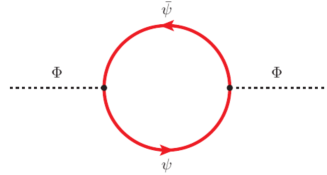
Figure 1: The one-loop self-energy of a neutral scalar $\Phi$ boson with an Yukawa interaction with a fermion field.

Given the interacting Lagrangian (8), the one-loop self-energy for $\Phi$ is given by the Feynman diagram shown in Fig. 1. Its explicit expression is given by

$$i\Pi(P) = (ig)^{2}\int\frac{d^{4}K}{(2\pi)^{4}}\mathrm{Tr}\left[S_{m}(-Q)S_{m}(K)\right],$$ (9)

where we have denoted $Q=P-K$ and $P$ is the external four-momentum.

Using the expression for the fermion propagator decomposed in terms of different Landau levels in presence of any arbitrary magnetic field given by Eq. (5), the self-energy becomes

$$i\Pi(P) = -g^{2}\int\frac{d^{4}K}{(2\pi)^{4}}~{}e^{-\frac{Q_{\perp}^{2}+K_{\perp}^{2}}{q_{f}B}}\sum_{n=0}^{+\infty}\sum_{m=0}^{+\infty}(-1)^{m+n}\left(\frac{\textsf{Tr}\left[D_{n}(q_{f}B,-Q)~{}D_{m}(q_{f}B,K)\right]}{(Q_{\shortparallel}^{2}-m_{f}^{2}-2nq_{f}B)(K_{\shortparallel}^{2}-m_{f}^{2}-2mq_{f}B)}\right),$$ (10)

where the expressions for $D_{n}$ is given by Eq. (6). The details of the derivation of Eq. (10) is given in the Appendix A. The final result can be expressed as

$$i\Pi(P_{\shortparallel}) = \frac{g^{2}q_{f}B}{\pi}\sum_{n=0}^{+\infty}(2-\delta_{n,0})\int\frac{d^{2}K_{\shortparallel}}{(2\pi)^{2}}~{}\frac{(K\cdot Q)_{\shortparallel}-m_{f}^{2}+4nq_{f}B}{(Q_{\shortparallel}^{2}-m_{f}^{2}-2nq_{f}B)(K_{\shortparallel}^{2}-m_{f}^{2}-2nq_{f}B)},$$ (11)

where we have set $P_{\perp}=0$ (we will mainly be interested in the expression for the decay width in the rest frame of the decaying scalar particle).

The imaginary part of the self-energy determines the decay width of the heavy boson, which in the onshell and rest frame of the decaying particle is defined as Peskin:1995ev

$$\Gamma_{M}=\frac{\mathrm{Im}~{}\Pi(P=M)}{M}.$$ (12)

Hence, by evaluating the imaginary part of Eq. (11) at finite temperature and in the presence of the external magnetic field, we obtain (see Appendix A)

$$\Gamma_{M}(B,T) = \frac{g^{2}q_{f}B}{2\pi M}\sum_{n=0}^{+\infty}(2-\delta_{n,0})\left(1-\frac{4m_{f}^{\prime 2}}{M^{2}}\right)^{{1}/{2}}\Theta\left(M^{2}-4m_{f}^{\prime 2}\right)\Bigl{[}1-2n_{F}\left(\frac{M}{2}\right)\Bigr{]}$$ (13)

$$+\frac{2g^{2}(q_{f}B)^{2}}{\pi M^{3}}\sum_{n=1}^{+\infty}n\left(1-\frac{4m_{f}^{\prime 2}}{M^{2}}\right)^{-{1}/{2}}\Theta\left(M^{2}-4m_{f}^{\prime 2}\right)\Bigl{[}1-2n_{F}\left(\frac{M}{2}\right)\Bigr{]},$$

where we have defined $m_{f}^{\prime 2}=m_{f}^{2}+2nq_{f}B$. The expression (13) gives the impression that it would diverge as we approach the threshold from above, $M\to 2m_{f}^{\prime+}$, but this is misleading. In fact, one notes that the kinematic constrain, set by the Heaviside function $\Theta\left(M^{2}-4m_{f}^{\prime 2}\right)$, implies that the sum is constrained up to a maximum value integer value $N_{\rm max}(B)$, given in terms of the magnetic field as

$$n<N_{\rm max}(B)={\rm Integer}\left[\frac{M^{2}-4m_{f}^{2}}{8q_{f}B}\right].$$ (14)

Explicitly, Eq. (13) then becomes

$$\Gamma_{M}(B,T) = \frac{\sqrt{2}g^{2}\left(q_{f}B\right)^{3/2}}{\pi M^{2}}\left[\sqrt{\frac{M^{2}-4m_{f}^{2}}{8q_{f}B}}\;\Theta\left(M^{2}-4m_{f}^{2}\right)\right.$$ (15)

$$+ \left.\sum_{n=1}^{N_{\rm max}(B)-1}\left(2\sqrt{\frac{M^{2}-4m_{f}^{2}}{8q_{f}B}-n}+\frac{1}{2}\frac{n}{\sqrt{\frac{M^{2}-4m_{f}^{2}}{8q_{f}B}-n}}\right)\right]\left[1-2n_{F}\left(\frac{M}{2}\right)\right],$$

where we have explicitly separated the LLL ($n=0$) term in the above expression. Note that for all the Landau levels with $n\geq 1$ the kinematic constrain implies that the magnetic field cannot be arbitrarily large without violating it. This determines a maximum value for the magnetic field, $q_{f}B_{\rm max}=(M^{2}-4m_{f}^{2})/8$, and for $B\geq B_{\rm max}$ we have that all terms in Eq. (15) with $n\geq 1$ vanishes and only the LLL terms contributes to the decay width.

III The weak and strong magnetic field limits for the scalar field decay width from the Yukawa coupling

Having computed the general expression for the decay width in the previous section, let us now focus on the approximation for the decay width in the cases of a strong and a weak magnetic field. These limiting cases are usually considered in the literature, so it is useful to analyze them as well for comparison. By weak and strong magnetic field here we mean $q_{f}B\ll m_{f}^{2}$ and $q_{f}B\gtrsim m_{f}^{2}$, respectively.

III.1 The weak magnetic field approximation

To consider the weak magnetic field, let us first consider the Dirac propagator in this case. Expanding the exponential and tangent functions in the expression Eq. (3), we immediately get $S_{m}(K)$ as a series in powers of $q_{f}B$. Up to order $(q_{f}B)^{2}$, it is expressed as

$$S_{mw}(K)=\frac{\not{K}+m_{f}}{K^{2}-m_{f}^{2}}+q_{f}B\frac{i(\not{K}_{\shortparallel}+m_{f})\gamma^{1}\gamma^{2}}{(K^{2}-m_{f}^{2})^{2}}+(q_{f}B)^{2}\left[\frac{2\not{K}_{\perp}}{(K^{2}-m_{f}^{2})^{3}}-\frac{2K_{\perp}^{2}(\not{K}+m_{f})}{(K^{2}-m_{f}^{2})^{4}}\right].$$ (16)

We can also write the above expression as

$$S_{mw}(K)=F(K,m_{f},m_{i})\frac{1}{K^{2}-m_{i}^{2}}\Bigg{|}_{m_{i}=m_{f}},$$ (17)

where

$$F=(\not{K}+m_{f})+i\,a_{j}\,\left(\not{K}_{\shortparallel}+m_{f}\right)\gamma^{1}\gamma^{2}+b_{j}\not{K}_{\perp}+c_{j}K_{\perp}^{2}(\not{K}+m_{f}),$$ (18)

with coefficients $a_{j},b_{j}$ and $c_{j}$ carrying the derivative operators,

$$a_{j}=q_{f}B\frac{\partial}{\partial m_{j}^{2}},~{}~{}b_{j}=(q_{f}B)^{2}\frac{\partial^{2}}{\partial(m_{j}^{2})^{2}},~{}~{}c_{j}=-\frac{1}{3}(q_{f}B)^{2}\frac{\partial^{3}}{\partial(m_{j}^{2})^{3}}.$$ (19)

The one-loop correlation function in this case is similarly given by

$$i\Pi_{w}(P) = (ig)^{2}\int\frac{d^{4}K}{(2\pi)^{4}}\mathrm{Tr}\left[S_{mw}(-Q)S_{mw}(K)\right]$$ (20)

$$= g^{2}\int\frac{d^{4}K}{(2\pi)^{4}}\left[{\cal N}_{a,b,c}\frac{1}{(Q^{2}-m_{1}^{2})(K^{2}-m_{2}^{2})}\right]\Bigg{|}_{m_{1}=m_{2}=m_{f}},$$

where

$${\cal N}_{a,b,c}=-\textrm{Tr}\left[F(K,m_{f},m_{2})~{}F(-Q,m_{f},m_{1})\right].$$ (21)

Here, the masses $m_{1}$ and $m_{2}$ are variables on which the mass derivatives inside ${\cal N}_{a_{j},b_{j},c_{j}}$ act on in the square bracket term in Eq. (20). Now, proceeding similarly as in the previous section, we can write down the imaginary part of the one-loop scalar self-energy for the decay process,

$$\textrm{Im}~{}\Pi_{w}(P) = \pi~{}g^{2}~{}\int\frac{d^{3}k}{(2\pi)^{3}}\frac{{\cal N}_{a,b,c}(\omega_{1},\omega_{2})~{}(1-n_{F}(\omega_{1})-n_{F}(\omega_{2}))}{4~{}\omega_{1}\omega_{2}}~{}\delta(p_{0}-\omega_{1}-\omega_{2})$$ (22)

where we have defined

$$\omega_{1}^{2} = q^{2}+m_{1}^{2},$$

$$\omega_{2}^{2} = k^{2}+m_{2}^{2}.$$

Let us evaluate the expression of ${\cal N}_{a,b,c}$ up to $\mathcal{O}(q_{f}B)^{2}$. First, consider the term inside the trace in Eq. (21),

$$F(K,m_{f},m_{2})~{}F(-Q,m_{f},m_{1}) = -\left[(\not{Q}-m_{f})+a_{1}~{}i~{}\left(\not{Q}_{\shortparallel}-m_{f}\right)\gamma^{1}\gamma^{2}+b_{1}\not{Q}_{\perp}+c_{1}Q_{\perp}^{2}(\not{Q}-m_{f})\right]$$ (23)

$$\times \left[(\not{K}+m_{f})+a_{2}~{}i~{}\left(\not{K}_{\shortparallel}+m_{f}\right)\gamma^{1}\gamma^{2}+b_{2}\not{K}_{\perp}+c_{2}K_{\perp}^{2}(\not{K}+m_{f})\right].$$

So,

$${\cal N}_{a,b,c} = -\textrm{Tr}\left[F(K,m_{f},m_{2})~{}F(-Q,m_{f},m_{1})\right]$$ (24)

$$= 4\left(1+c_{1}Q_{\perp}^{2}+c_{2}K_{\perp}^{2}\right)\left(K\cdot Q-m_{f}^{2}\right)+4a_{1}a_{2}\left((K\cdot Q)_{\shortparallel}-m_{f}^{2}\right)$$

$$+~{}4(b_{1}+b_{2})\left(K\cdot Q\right)_{\perp}.$$

Now neglecting the external transverse momentum $P_{\perp}$, in turn we obtain

$${\cal N}_{a,b,c}(\omega_{1},\omega_{2}) = 4(1+a_{1}a_{2}+(c_{1}+c_{2})K_{\perp}^{2})(K\cdot Q-m_{f}^{2})-4(a_{1}a_{2}+b_{1}+b_{2})K_{\perp}^{2}$$ (25)

$$= 4\left(1+a_{1}a_{2}+\frac{2}{3}(c_{1}+c_{2})k^{2}\right)(K\cdot Q-m_{f}^{2})-\frac{8}{3}(a_{1}a_{2}+b_{1}+b_{2})k^{2},$$

where we have also taken $K_{\perp}^{2}=k^{2}\left\langle\sin^{2}\theta\right\rangle_{\theta}=\frac{2}{3}k^{2}$, an approximation exploiting the choice of the frame which is valid in the weak field limit.

So, the decay width in the rest frame of the decaying boson for the weakly magnetized medium is given by

$$\Gamma^{\textrm{w}} = \frac{\mathrm{Im}~{}\Pi_{w}}{M}$$ (26)

$$= \left[\frac{4\pi g^{2}}{M}(1+a_{1}a_{2})~{}J_{1}+\frac{8\pi g^{2}}{3M}(c_{1}+c_{2})~{}J_{2}-\frac{8\pi g^{2}}{3M}(a_{1}a_{2}+b_{1}+b_{2})~{}J_{3}\right]\Bigg{|}_{m_{1}=m_{2}=m_{f}},$$

where

$$J_{1} = \int\frac{d^{3}k}{(2\pi)^{3}}\left(K\cdot Q-m_{f}^{2}\right)\frac{\left[1-n_{F}(\omega_{1})-n_{F}(\omega_{2})\right]}{4\omega_{1}\omega_{2}}\delta(p_{0}-\omega_{1}-\omega_{2}),$$ (27)

$$J_{2} = \int\frac{d^{3}k}{(2\pi)^{3}}~{}k^{2}\left(K\cdot Q-m_{f}^{2}\right)\frac{\left[1-n_{F}(\omega_{1})-n_{F}(\omega_{2})\right]}{4\omega_{1}\omega_{2}}\delta(p_{0}-\omega_{1}-\omega_{2}),$$ (28)

$$J_{3} = \int\frac{d^{3}k}{(2\pi)^{3}}~{}k^{2}\frac{\left[1-n_{F}(\omega_{1})-n_{F}(\omega_{2})\right]}{4\omega_{1}\omega_{2}}\delta(p_{0}-\omega_{1}-\omega_{2}).$$ (29)

In the Appendix B we derive the respective expressions for Eqs. (27), (28) and (29). Proceeding with the final momentum integrations in the scalar field rest frame, we obtain that

$$\Gamma^{\textrm{w}}_{M}(T,B)=\Gamma^{\textrm{w}}_{M}(T=0,B)\left[1-2n_{F}\left(\frac{M}{2}\right)\right],$$ (30)

where

$$\Gamma^{\textrm{w}}_{M}(T=0,B) = \frac{g^{2}M}{8\pi}\left(1-\frac{4m_{f}^{2}}{M^{2}}\right)^{3/2}\Theta\left(M^{2}-4m_{f}^{2}\right)$$ (31)

$$\times \left[1-\frac{2(q_{f}B)^{2}}{M^{4}}\left(\frac{8}{3}-\frac{2m_{f}^{2}}{M^{2}}\right)\left(1-\frac{4m_{f}^{2}}{M^{2}}\right)^{-2}\right].$$

Note that the first term on the right hand side of the above expression can be identified as the usual vacuum decay width $\Gamma^{\textrm{v}}_{M}$, when evaluated at $B=0$.

III.2 The strong magnetic field approximation

Let us now obtain the limiting case of the decay width in a strong magnetic field, in particular when $q_{f}B\gg m_{f}^{2}$. In presence of a very strong magnetic field all the Landau levels with $n\geq 1$ are pushed to infinity compared to the lowest Landau Level (LLL) with $n=0$. So, for the case of strong external magnetic field we can assume the LLL approximation, by the virtue of which the fermion propagator in Eq. (5) reduces to a simplified form as

$$iS_{ms}(K)=ie^{-{K_{\perp}^{2}}/{q_{f}B}}~{}~{}\frac{\not{K}_{\shortparallel}+m_{f}}{K_{\shortparallel}^{2}-m_{f}^{2}}(1-i\gamma_{1}\gamma_{2}),$$ (32)

where $K$ is four-momentum and we have used the properties of the generalized Laguerre polynomial, $L_{n}\equiv L_{n}^{0}$ and $L_{-1}^{\alpha}=0$. The one-loop scalar self-energy can then be written as

$$i\Pi_{LLL}(P) = g^{2}\int\frac{d^{2}K_{\perp}}{(2\pi)^{2}}\exp\left(\frac{-K_{\perp}^{2}-Q_{\perp}^{2}}{q_{f}B}\right)$$ (33)

$$\times \int\frac{d^{2}K_{\shortparallel}}{(2\pi)^{2}}~{}\mathrm{Tr}\left[\frac{\not{Q}_{\shortparallel}-m_{f}}{Q_{\shortparallel}^{2}-m_{f}^{2}}(1-i\gamma_{1}\gamma_{2})\frac{\not{K}_{\shortparallel}+m_{f}}{K_{\shortparallel}^{2}-m_{f}^{2}}(1-i\gamma_{1}\gamma_{2})\right].$$

Evaluation of the trace and the Gaussian integral over $K_{\perp}$ in Eq. (33) is rather straightforward, which yields

$$i\Pi_{LLL}(P) = g^{2}\frac{q_{f}B}{\pi}\exp\left(\frac{-P_{\perp}^{2}}{2q_{f}B}\right)\int\frac{d^{2}K_{\shortparallel}}{(2\pi)^{2}}~{}\frac{(K\cdot Q)_{\shortparallel}-m_{f}^{2}}{(Q_{\shortparallel}^{2}-m_{f}^{2})(K_{\shortparallel}^{2}-m_{f}^{2})},$$ (34)

$$= ig^{2}\frac{q_{f}B}{\pi}\exp\left(\frac{-P_{\perp}^{2}}{2q_{f}B}\right)~{}I_{1,LLL},$$

where $I_{1,LLL}$ is the same momentum integral we have already computed in the Appendix A and given by Eq. (69) when it is evaluated by considering only the LLL term, i.e., by taking $m_{f}^{\prime}\to m_{f}$ in there. Hence, the imaginary part of the one-loop scalar field self-energy in the LLL approximation becomes

$$\mathrm{Im}~{}\Pi_{LLL}(P) = g^{2}\frac{q_{f}B}{\pi}\exp\left(\frac{-P_{\perp}^{2}}{2q_{f}B}\right)~{}\mathrm{Im}~{}I_{1}(m_{f}^{\prime}\to m_{f})$$ (35)

$$= g^{2}\frac{q_{f}B}{2\pi}~{}e^{\frac{-P_{\perp}^{2}}{2q_{f}B}}\left(1-\frac{4m_{f}^{2}}{P_{\shortparallel}^{2}}\right)^{\frac{1}{2}}\Theta\left(P_{\shortparallel}^{2}-4m_{f}^{2}\right)\Bigl{[}1-n_{F}(p_{+}^{s})-n_{F}(p_{-}^{s})\Bigr{]},$$

where

$$p_{\pm}^{s}=\frac{p_{0}}{2}\pm\frac{p_{3}}{2}\sqrt{1-\frac{4m_{f}^{2}}{P_{\shortparallel}^{2}}}$$ (36)

and the decay width in the rest frame of the decaying scalar, in presence of a strong background magnetic field and in the LLL approximation is given by

$$\Gamma_{M,LLL} = \frac{\mathrm{Im}~{}\Pi_{LLL}(P=M)}{M}$$ (37)

$$= g^{2}\frac{q_{f}B}{2\pi M}~{}\left(1-\frac{4m_{f}^{2}}{M^{2}}\right)^{{1}/{2}}\Bigl{[}1-2n_{F}\left(\frac{M}{2}\right)\Bigr{]}\Theta\left(M^{2}-4m_{f}^{2}\right).$$

Equation (37) can also be verified by putting $n=0$ in Eq. (13).

IV Discussion of the results

Let us now compare the results we have obtained for the decay width in the previous sections. We start by comparing the arbitrary field result given by Eq. (15) with the two approximating expressions from the latter section, i.e., the weak field approximation given by Eq. (30) and the strong field approximation given by Eq. (37). This is shown in Fig. 2. For convenience, we normalize the results by the decay width in the absence of an external magnetic field,

$$\Gamma_{M}(B=0)=\frac{g^{2}M}{8\pi}\left(1-\frac{4m_{f}^{2}}{M^{2}}\right)^{3/2}\left[1-2n_{F}\left(\frac{M}{2}\right)\right]\Theta\left(M^{2}-4m_{f}^{2}\right).$$ (38)

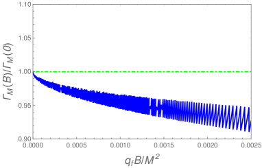
(a) The weak field case

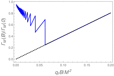
(b) The strong field case

Figure 2: The decay width (normalized by the magnetic field independent result), as a function of the magnetic field. The solid lines in both (a) and (b) are the result of Eq. (15), the dotted line in (b) is the strong field result Eq. (37) and the dash-dotted line in (a) is the weak field approximation Eq. (30). We have set the fermion mass as $m_{f}=M/20$.

From the results of Fig. 2 we can see that the general behavior of the decay width is to decrease with the magnetic field. The sharp teeth-saw behavior is consequence of the discretized Landau levels in Eq. (15). Within each Landau level, the decay width tends to increase, till the kinematical constrain is reached and we begin again with the next Landau level, which gives origin to the teeth-saw behavior seen in Fig. 2. Note that the highest Landau levels are populated initially at lowest values of $B$, with the LLL populated for very last at the highest value of $B$, before the decay width eventually vanishes for all Landau levels with $n\geq 1$ due to the kinematic constrain, remaining only the LLL contribution. The weak magnetic field also shows a decrease with the magnetic field, though barely apparent in the scale of Fig. 2a, where we show it only up to its range of validity. In particular, we see that at the value $q_{f}B=m_{f}^{2}$ the weak field approximation already over estimates the decay width by around $5\%$ compared to the arbitrary field result. The strong field approximation, expressed in Eq. (37) and shown as the dotted line in Fig. 2b, has always an increasing (linear in $B$) behavior with the magnetic field. This can be better seen by noticing that the sum over the Landau levels in Eq. (15) has an explicit analytic continuation in terms of zeta-functions,

$$\Gamma_{M}(B,T) = \frac{\sqrt{2}g^{2}\left(q_{f}B\right)^{3/2}}{\pi M^{2}}\sqrt{\frac{M^{2}-4m_{f}^{2}}{8q_{f}B}}\Theta\left(M^{2}-4m_{f}^{2}\right)$$ (39)

$$+ \frac{\sqrt{2}g^{2}\left(q_{f}B\right)^{3/2}}{\pi M^{2}}\left[-\frac{3}{2}\zeta\left(-\frac{1}{2},\frac{M^{2}-4m_{f}^{2}}{8q_{f}B}\right)\right.$$

$$- \left.\frac{N_{\rm max}(B)}{2}\zeta\left(\frac{1}{2},\frac{M^{2}-4m_{f}^{2}}{8q_{f}B}\right)+\frac{3}{2}\zeta\left(-\frac{1}{2}\right)+\frac{M^{2}-4m_{f}^{2}}{16q_{f}B}\zeta\left(\frac{1}{2}\right)\right]$$

$$\times \left[1-2n_{F}\left(\frac{M}{2}\right)\right]\Theta\left[N_{\rm max}(B)-1\right],$$

where in the above expression we have again separated explicitly the LLL $n=0$ contribution, while explicitly summing over the $n\geq 1$ Landau levels and

$$\zeta(s,a)=\sum_{k=0}^{\infty}\frac{1}{(k+a)^{s}},$$ (40)

is the Hurwitz zeta function zeta .

In Fig. 3 we compare the result given by Eq. (15) with the analytic continuation of it in terms of the zeta-functions.

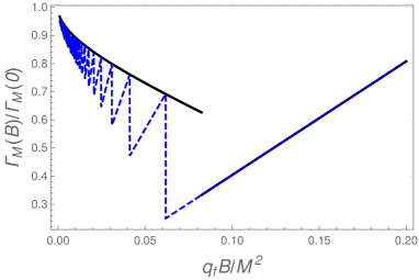
Figure 3: The decay width (normalized by the magnetic field independent result), as a function of the magnetic field. The dashed line is the zeta-function analytic continuation given by Eq. (39), while the solid line is Eq. (15). We have set the fermion mass as $m_{f}=M/20$.

The analytic continuation result given by Eq. (39) makes it clearer that the decay width is always a decreasing function with the magnetic field, except, of course, at the threshold point, where the decay width contribution with Landau levels with $n\geq 1$ vanishes and only remains the LLL contribution, that now grows linearly with $B$.

V Bosonic decay in the presence of an arbitrary magnetic field

Let us now consider the case of decay of a heavy neutral scalar field into a pair of charged scalars, $\Phi\to\chi+\chi^{*}$. The interacting Lagrangian density is given by the trilinear coupling between the fields,

$$\mathcal{L}=g\Phi\chi^{*}\chi.$$ (41)

The scalar field $\Phi$ self-energy is now given by

$$i\Pi^{b}(P)=(ig)^{2}\int\frac{d^{4}K}{(2\pi)^{4}}D_{B}(P-K)D_{B}(K),$$ (42)

where $D_{B}(K)$ is the bosonic propagator in presence of an arbitrary external magnetic field and it is given by Ayala:2004dx

$$D_{B}(K)=2\sum\limits_{n=0}^{\infty}\frac{(-1)^{n}L_{n}\left(\frac{2K_{\perp}^{2}}{q_{b}B}\right)~{}e^{-\frac{K_{\perp}^{2}}{q_{b}B}}}{K_{\shortparallel}^{2}-(2n+1)q_{b}B-m_{b}^{2}+i\epsilon},$$ (43)

where $q_{b}$ is the bosonic charge. Incorporating this expression for the bosonic propagator and neglecting the external transverse momentum $P_{\perp}$ again, it allows us to obtain an analytic result for the self-energy, which becomes

$$i\Pi^{b}(P_{\shortparallel})=-4g^{2}\!\!\int\!\!\frac{d^{2}K_{\shortparallel}}{(2\pi)^{2}}\!\!\int\!\!\frac{d^{2}K_{\perp}}{(2\pi)^{2}}\!\!\sum_{l,n=0}^{+\infty}\!\!\!(-1)^{l+n}e^{-\frac{2K_{\perp}^{2}}{q_{b}B}}L_{l}\!\left(\!\frac{2K_{\perp}^{2}}{q_{b}B}\!\right)\!L_{n}\!\left(\!\frac{2K_{\perp}^{2}}{q_{b}B}\!\right)\!\frac{1}{(K_{\shortparallel}^{2}-m_{b}^{\prime 2})(Q_{\shortparallel}^{2}-m_{b}^{\prime\prime 2})},$$ (44)

where we have used $Q\equiv P-K$ with $m_{b}^{\prime 2}=m_{b}^{2}+(2n+1)q_{b}B$ and $m_{b}^{\prime\prime 2}=m_{b}^{2}+(2l+1)q_{b}B$.

Now, using the same orthogonality relation as used in Eq. (66), we obtain

$$\Pi^{b}(P) = 4ig^{2}\frac{q_{b}B}{8\pi}\sum_{n=0}^{+\infty}\int\frac{d^{2}K_{\shortparallel}}{(2\pi)^{2}}\frac{1}{(K_{\shortparallel}^{2}-m_{b}^{\prime 2})(Q_{\shortparallel}^{2}-m_{b}^{\prime 2})},$$ (45)

where now

$$\int\frac{d^{2}K_{\shortparallel}}{(2\pi)^{2}}\to iT\sum_{j}\int\frac{dk_{3}}{2\pi},$$ (46)

and the Minkowski time component of the momentum is replaced by $k_{0}\to i\omega_{j}$, where $\omega_{j}=2j\pi T$, $j=0,\pm 1,\ldots$, are the Matsubara’s frequencies for bosons.

Similarly as the fermionic loop derivation done in Appendix A, we can perform the resulting Matsubara sum in the bosonic loop by using again the mixed representation technique prescribed by Pisarski Pisarski:1987wc ; Bandyopadhyay:2016fyd , but this time for bosons,

$$\frac{1}{K_{\shortparallel}^{2}-m_{b}^{2}}\equiv\frac{1}{k_{0}^{2}-E_{k}^{2}}=\int\limits_{0}^{1/T}d\tau e^{k_{0}\tau}\Delta_{M}(\tau,k),$$ (47)

where

$$\Delta_{M}(\tau,k)=\frac{1}{2E_{k}}\left\{\left[1+n_{B}(E_{k})\right]e^{-E_{k}\tau}+n_{B}(E_{k})e^{E_{k}\tau}\right\},$$ (48)

where we have defined the dispersion relation as $E_{k}^{2}=k_{3}^{2}+m_{b}^{\prime 2}$ and $n_{B}(E_{k})$ in the above equation is the Bose-Einstein distribution function. This way, we get for the Masubara’s sum for the bosonic loop the result

$$T\sum_{k_{0}}\frac{1}{(k_{0}^{2}-E_{k}^{2})(q_{0}^{2}-E_{q}^{2})}=\sum\limits_{r,l=\pm 1}\frac{rl}{4E_{k}E_{q}}~{}\frac{1+n_{B}(rE_{k})+n_{B}(lE_{q})}{(p_{0}+rE_{k}+lE_{q})},$$ (49)

We now proceed similarly as in the derivation for the discontinuity of the fermionic loop that determines the decay width. Using Eq. (75) to evaluate the discontinuity and being interested only in the contribution from decay (and not Landau damping), we can choose $r=l=-1$ in Eq. (49). Then, by also using Eq. (78) to perform the $k_{3}$ integration, we finally obtain that

$$\mathrm{Im}~{}\Pi^{b}(P_{\shortparallel}) = \frac{g^{2}q_{b}B}{4\pi}\sum_{n=0}^{+\infty}\Theta(P_{\shortparallel}^{2}-4m_{b}^{\prime 2})\left(1-\frac{4m_{b}^{\prime 2}}{P_{\shortparallel}^{2}}\right)^{-\frac{1}{2}}\frac{1}{P_{\shortparallel}^{2}}\left[1+n_{B}(p_{+}^{b})+n_{B}(p_{-}^{b})\right],$$ (50)

where

$$p_{\pm}^{b}=\frac{p_{0}}{2}\pm\frac{p_{3}}{2}\sqrt{\left(1-\frac{4m_{b}^{\prime 2}}{P_{\shortparallel}^{2}}\right)}.$$ (51)

Thus, the one-loop decay width for the process $\Phi\to\chi+\chi^{*}$, in the rest frame of the decaying heavy scalar, becomes

$$\Gamma_{M}^{b}(B,T) = \frac{\mathrm{Im}~{}\Pi(P_{\shortparallel}=M)}{M}$$ (52)

$$= \frac{g^{2}q_{b}B}{4\pi M^{3}}\sum_{n=0}^{+\infty}\Theta(M^{2}-4m_{b}^{\prime 2})\left(1-\frac{4m_{b}^{\prime 2}}{M^{2}}\right)^{-\frac{1}{2}}\left[1+2n_{B}\left(\frac{M}{2}\right)\right].$$

As in the fermionic loop case, the kinematic constrain in Eq. (52) limits the upper value for the Landau levels such that

$$n<{\rm Integer}\left[\frac{M^{2}-4m_{b}^{2}}{8q_{b}B}-\frac{1}{2}\right]\equiv N_{\rm max,b}(B),$$ (53)

and Eq. (52) becomes

$$\Gamma_{M}^{b}(B,T) = \frac{g^{2}q_{b}B}{4\pi M^{3}}\sum_{n=0}^{N_{\rm max,b}(B)-1}\left\{1-\frac{4\left[m_{b}^{2}+(2n+1)q_{b}B\right]}{M^{2}}\right\}^{-\frac{1}{2}}\left[1+2n_{B}\left(\frac{M}{2}\right)\right].$$ (54)

The above expression also has an analytic continuation in terms of zeta-functions, given by

$$\Gamma_{M}^{b}(B,T) = \frac{\sqrt{2}g^{2}\sqrt{q_{b}B}}{16\pi M^{2}}\left[\zeta\left(\frac{1}{2}\right)-\zeta\left(\frac{1}{2},\frac{M^{2}-4m_{b}^{2}}{8q_{b}B}+\frac{1}{2}\right)\right]\left[1+2n_{B}\left(\frac{M}{2}\right)\right]\Theta\left(N_{\rm max,b}(B)-1\right).$$ (55)

The above expression for the arbitrary magnetic field can be compared with the corresponding limiting results for the bosonic decay width. In the weak field approximations, which was derived in details in Ref. Piccinelli:2017yvl , the decay width is given by

$$\Gamma_{M,{\rm weak}}^{b}(B,T) \simeq \frac{g^{2}}{16\pi M^{2}}\sqrt{1-4\frac{m_{b}^{2}}{M^{2}}}\left[1+2n_{B}\left(\frac{M}{2}\right)\right]\Theta(M^{2}-4m_{b}^{2})$$ (56)

$$\times \left[1-\frac{2(q_{b}B)^{2}}{3M^{4}}\left(1-40\frac{m_{b}^{2}}{M^{2}}\right)\right].$$

Likewise, we can easily determine the strong field approximation, given by the LLL contribution,

$$\Gamma_{M,LLL}^{b}(B,T) = \frac{g^{2}q_{b}B}{4\pi M^{3}}\left[1-\frac{4\left(m_{b}^{2}+q_{b}B\right)}{M^{2}}\right]^{-\frac{1}{2}}\left[1+2n_{B}\left(\frac{M}{2}\right)\right]\Theta(M^{2}-4m_{b}^{2}),$$ (57)

and also subject to the range of applicability (following from Eq. (53) and that $m_{b}^{2}<q_{b}B$),

$$1-4\frac{m_{b}^{2}+q_{b}B}{M^{2}}>8\frac{q_{b}B}{M^{2}}>8\frac{m_{b}^{2}}{M^{2}}.$$ (58)

The largest range still comes when we set the boson mass to zero, with the magnetic field then limited by the maximum value $q_{b}B<M^{2}/12$, thus, smaller than the equivalent condition found for the case of the decay into fermions.

In Fig. 4 we compare the different results shown above. As in the fermionic decay case, we have normalized the decay width by the zero magnetic field result, given by

$$\Gamma_{M}^{b}(B=0,T) = \frac{g^{2}}{16\pi M}\left(1-\frac{4m_{b}^{2}}{M^{2}}\right)^{1/2}\left[1+2n_{B}\left(\frac{M}{2}\right)\right]\Theta\left(M^{2}-4m_{b}^{2}\right).$$ (59)

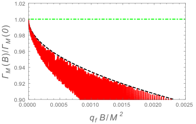
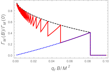
Figure 4: The decay width (normalized by the magnetic field independent result), as a function of the magnetic field for the case of a decay of a heavy neutral scalar field into charged ones. The dashed line is the result of Eq. (55), the solid line is given by Eq. (54), the dash-dotted line is the weak field result given Eq. (56) and the dotted line is the strong field approximation Eq. (57). We have set the charged boson mass as $m_{b}=M/20$.

In Fig. 4, the sharp teeth-saw behavior is again consequence of the discrete Landau levels considered in Eq. (54). We also note in Fig. 4a that the weak field approximation now over estimates the exact result by a much larger percentage, as compared, e.g., to the decay into fermions case. Furthermore, we see from Fig. 4b that, as in the fermionic decay case, the LLL approximation predicts always an increasing decay width with the magnetic field, while the analytic full result is always decreasing with the magnetic field. Contrary to the case of the decay into fermions where at large magnetic fields only the LLL contributions survives, in the case of decay into bosonic particles the kinematic constrain forces even the LLL term to vanish. This is simply a consequence that the dispersion relation for bosons depends explicitly on $B$ even when $n=0$.

VI Conclusions

In this work, we have studied the decay channels of a heavy neutral scalar field into a pair of fermion-antifermion and a pair of charged scalars when in the presence of an external magnetic field. Our results indicate that there are similarities in these two decay channels as a function of the magnetic field. In both the cases, we observe that the decay width always tends to decrease with the increase in the magnetic field up to the point where the LLL is filled. In a sense, this behavior could be anticipated by the fact that in presence of a magnetic field the effective mass of the decay products (as perceived by the decaying particle) increases with the intensity of the magnetic field. This can be seen easily when we look at the dispersion relation for a charged scalar for example.

We have compared our analytical results, which can also be expressed in an analytic continuation using zeta-functions, with the approximated results in the limiting regimes, i.e., in the weak field approximation (where the magnetic field satisfies $qB\ll m^{2}$) and in the strong field or LLL approximation, where $qB\geq m^{2}$. We have seen that the kinematic condition leads to a natural constrain in the upper magnitude of the external magnetic field, beyond which the contribution of all the Landau levels with $n\geq 1$ to decay width vanishes. In the case of decay into fermions only the LLL contribution remains and make the decay width to grow linearly with $B$. For the decay into bosons, however, even the LLL vanishes as a consequence of the kinematic constrain and that it now depends explicitly on $B$ even for the LLL. When contrasting both results with the analytic expressions, we see that the weak field approximation tends to over estimate the decay width. The strong field approximation, on the other hand, leads to a complete wrong behavior of the decay width in the decay into bosons case, showing a monotonic increase with $B$. These results point out that the use of these approximations in the literature should be seen with quite some reservations.

We find that the decay width in strong magnetic fields is entirely blocked in the case of decay into bosons. This behavior is different to what we see from the behavior of the decay widths when in the presence of temperature or chemical potential. For instance, the dependence on the temperature seen in the case of the decay into fermions, given by Eq. (15), is a consequence of the decrease of the phase space for the decay process as we increase the temperature (i.e., Pauli blocking). In the case of the decay into bosons, the phase space increases due the bosonic nature of the statistics, thus increasing the decay width with the temperature. The decrease of the decay width with the magnetic field and its blocking at larger values of the external field is essentially a consequence of the kinematic condition given its explicitly dependence on $B$. It would be interesting to study the case where higher-loop effects are accounted for, or when the decaying particle is also charged under the external magnetic field. In this case, the dressing of the masses by magnetic field dependent terms might lead to nontrivial effects.

The results obtained in this work can find many different applications. For instance the blocking of the decay in strong magnetic field can have many important consequences. Possible applications can be found in the context of early Universe where conditions predict the presence of extreme magnetic fields Vachaspati:1991nm ; Giovannini:2003yn ; Piccinelli:2014dya . In particular, the study of how external conditions might affect decay widths are of particular importance to understand the dynamics that might be in play in cosmology BasteroGil:2010pb . It is also known that the presence of an external magnetic field can influence the order of phase transitions Ayala:2004dx ; Duarte:2011ph . By also influencing the decay processes happening in these phase transitions, this can be potentially important in the problem of baryogenesis in the early Universe. In addition to this, another situation that our results can be applicable is the study of the decay processes following a heavy-ion collision, or, same in the presence of the extreme fields in magnetars. In heavy-ion collision experiments, our results can be applicable in the study of the decay of the neutral pion into quarks. Our findings can be applicable and be also of relevance in the study of the processes involving the decay of the Higgs into charged leptons, or, for the case of extensions of the Standard Model, in the study of the decay of other scalar particles into charged ones.

Appendix A The fermion loop term

We start this section by evaluating the trace term appearing in Eq. (10). It can be expressed in the form

$$\textsf{Tr}\left[D_{n}(q_{f}B,-Q)~{}D_{m}(q_{f}B,K)\right]=T_{1}+T_{2}+T_{3},$$ (60)

where the terms $T_{1}$, $T_{2}$ and $T_{3}$ are defined as

$$T_{1} = L_{n}\left(\frac{2Q_{\perp}^{2}}{q_{f}B}\right)L_{m}\left(\frac{2K_{\perp}^{2}}{q_{f}B}\right)$$ (61)

$$\times \textsf{Tr}\Bigl{[}-\left(q_{0}\gamma_{0}-q_{3}\gamma_{3}-m_{f}\right)\left(1-i\gamma_{1}\gamma_{2}\right)\left(k_{0}\gamma_{0}-k_{3}\gamma_{3}+m_{f}\right)\left(1-i\gamma_{1}\gamma_{2}\right)\Bigr{]}$$

$$= -8\left[(K\cdot Q)_{\shortparallel}-m_{f}^{2}\right]L_{n}\left(\frac{2Q_{\perp}^{2}}{q_{f}B}\right)L_{m}\left(\frac{2K_{\perp}^{2}}{q_{f}B}\right),$$

$$T_{2} = L_{n-1}\left(\frac{2Q_{\perp}^{2}}{q_{f}B}\right)L_{m-1}\left(\frac{2K_{\perp}^{2}}{q_{f}B}\right)$$ (62)

$$\times \textsf{Tr}\Bigl{[}-\left(q_{0}\gamma_{0}-q_{3}\gamma_{3}-m_{f}\right)\left(1+i\gamma_{1}\gamma_{2}\right)\left(k_{0}\gamma_{0}-k_{3}\gamma_{3}+m_{f}\right)\left(1+i\gamma_{1}\gamma_{2}\right)\Bigr{]}$$

$$= -8\left[(K\cdot Q)_{\shortparallel}-m_{f}^{2}\right]L_{n-1}\left(\frac{2Q_{\perp}^{2}}{q_{f}B}\right)L_{m-1}\left(\frac{2K_{\perp}^{2}}{q_{f}B}\right),$$

$$T_{3} = 16L_{n-1}^{1}\left(\frac{2Q_{\perp}^{2}}{q_{f}B}\right)L_{m-1}^{1}\left(\frac{2K_{\perp}^{2}}{q_{f}B}\right)\textsf{Tr}\Bigl{[}-\left(q_{1}\gamma_{1}+q_{2}\gamma_{2}\right)\left(k_{1}\gamma_{1}+k_{2}\gamma_{2}\right)\Bigr{]}$$ (63)

$$= 64(K\cdot Q)_{\perp}L_{n-1}^{1}\left(\frac{2Q_{\perp}^{2}}{q_{f}B}\right)L_{m-1}^{1}\left(\frac{2K_{\perp}^{2}}{q_{f}B}\right).$$

Here we note that the cross terms appearing in the expression of $D_{n}(q_{f}B,-Q)~{}D_{m}(q_{f}B,K)$, e.g. $L_{n}()~{}L_{m-1}()$ or $L_{n}()~{}L^{1}_{m-1}()$, vanish while evaluating the trace due to the properties of the associated gamma matrices. In the following, we also work with the case of a vanishing external transverse momentum, $P_{\perp}=0$, such that the expression for the self-energy Eq. (10) then becomes

$$\Pi(P_{\shortparallel}) = -ig^{2}\int\frac{d^{2}K_{\shortparallel}}{(2\pi)^{2}}\int\frac{d^{2}K_{\perp}}{(2\pi)^{2}}~{}e^{-\frac{2K_{\perp}^{2}}{q_{f}B}}\sum_{n=0}^{\infty}\sum_{m=0}^{\infty}\left(\frac{(-1)^{m+n}}{Q_{\shortparallel}^{2}-m_{f}^{2}-2nq_{f}B}\right)\left(\frac{1}{K_{\shortparallel}^{2}-m_{f}^{2}-2mq_{f}B}\right)$$ (64)

$$\times\Biggl{[}8\left((K\cdot Q)_{\shortparallel}-m_{f}^{2}\right)\left\{L_{n}\left(\frac{2K_{\perp}^{2}}{q_{f}B}\right)L_{m}\left(\frac{2K_{\perp}^{2}}{q_{f}B}\right)+L_{n-1}\left(\frac{2K_{\perp}^{2}}{q_{f}B}\right)L_{m-1}\left(\frac{2K_{\perp}^{2}}{q_{f}B}\right)\right\}$$

$$+64K_{\perp}^{2}L_{n-1}^{1}\left(\frac{2K_{\perp}^{2}}{q_{f}B}\right)L_{m-1}^{1}\left(\frac{2K_{\perp}^{2}}{q_{f}B}\right)\Biggr{]}.$$

Now, to integrate the transverse part out, we use the orthogonality relation of the Laguerre polynomials,

$$\int\limits_{0}^{\infty}x^{\alpha}e^{-x}L_{n}^{\alpha}(x)L_{m}^{\alpha}(x)dx=\frac{\Gamma(n+\alpha+1)}{n!}\delta_{n,m}.$$ (65)

Thus, we have that

$$\int\limits_{0}^{\infty}e^{-\frac{2K_{\perp}^{2}}{q_{f}B}}L_{n}\left(\frac{2K_{\perp}^{2}}{q_{f}B}\right)L_{m}\left(\frac{2K_{\perp}^{2}}{q_{f}B}\right)\frac{d^{2}K_{\perp}}{(2\pi)^{2}} = \frac{q_{f}B}{8\pi}~{}\delta_{n,m},$$ (66)

$$\int\limits_{0}^{\infty}K_{\perp}^{2}~{}e^{-\frac{2K_{\perp}^{2}}{q_{f}B}}L_{n-1}^{1}\left(\frac{2K_{\perp}^{2}}{q_{f}B}\right)L_{m-1}^{1}\left(\frac{2K_{\perp}^{2}}{q_{f}B}\right)\frac{d^{2}K_{\perp}}{(2\pi)^{2}} = \frac{(q_{f}B)^{2}}{16\pi}~{}n\,\delta_{n,m}.$$ (67)

After integrating out the transverse part using these orthogonality relations and using the Kronecker delta-functions we are then left with the result for the self-energy,

$$\Pi(P_{\shortparallel}) = -ig^{2}\int\frac{d^{2}K_{\shortparallel}}{(2\pi)^{2}}\left[\frac{q_{f}B}{\pi}\sum_{n=0}^{+\infty}(2-\delta_{n,0})\frac{(K\cdot Q)_{\shortparallel}-m_{f}^{\prime 2}}{(Q_{\shortparallel}^{2}-m_{f}^{\prime 2})(K_{\shortparallel}^{2}-m_{f}^{\prime 2})}\right.$$ (68)

$$\left.~{}~{}~{}~{}~{}~{}~{}~{}~{}~{}+8\frac{(q_{f}B)^{2}}{\pi}\sum_{n=1}^{+\infty}\frac{n}{(Q_{\shortparallel}^{2}-m_{f}^{\prime 2})(K_{\shortparallel}^{2}-m_{f}^{\prime 2})}\right],$$

where we have defined $m_{f}^{\prime 2}=m_{f}^{2}+2nq_{f}B$.

Let us call the first momentum integral in Eq. (68) as

$$I_{1}(P_{\shortparallel})=\int\frac{d^{2}K_{\shortparallel}}{(2\pi)^{2}}\frac{(K\cdot Q)_{\shortparallel}-m_{f}^{\prime 2}}{(Q_{\shortparallel}^{2}-m_{f}^{\prime 2})(K_{\shortparallel}^{2}-m_{f}^{\prime 2})},$$ (69)

and the second momentum integral in Eq. (68) as

$$I_{2}(P_{\shortparallel})=\int\frac{d^{2}K_{\shortparallel}}{(2\pi)^{2}}\frac{1}{(Q_{\shortparallel}^{2}-m_{f}^{\prime 2})(K_{\shortparallel}^{2}-m_{f}^{\prime 2})}.$$ (70)

At finite temperature, we can replace the momentum integral in the above equations by

$$\int\frac{d^{2}K_{\shortparallel}}{(2\pi)^{2}}\to iT\sum_{j}\int\frac{dk_{3}}{2\pi},$$ (71)

and the Minkowski time component of the momentum is replaced by $k_{0}\to i\omega_{j}$, where $\omega_{j}=(2j+1)\pi T$, $j=0,\pm 1,\ldots$, are the Matsubara’s frequencies for fermions.

Working first with the momentum integral $I_{1}$, we can now perform the Matsubara sum in $I_{1}$ by using the mixed representation technique prescribed by Pisarski Pisarski:1987wc ; Bandyopadhyay:2016fyd . In this prescription, we have that

$$\frac{1}{K_{\shortparallel}^{2}-m_{f}^{\prime 2}}\equiv\frac{1}{k_{0}^{2}-E_{k}^{2}}=\int\limits_{0}^{1/T}d\tau e^{k_{0}\tau}\Delta_{M}(\tau,k),$$ (72)

where

$$\Delta_{M}(\tau,k)=\frac{1}{2E_{k}}\left\{\left[1-n_{F}(E_{k})\right]e^{-E_{k}\tau}-n_{F}(E_{k})e^{E_{k}\tau}\right\},$$ (73)

where we have defined the dispersion relation as $E_{k}^{2}=k_{3}^{2}+m_{f}^{\prime 2}$ and $n_{F}(E_{k})$ in the above equation is the Fermi-Dirac distribution function. Using this technique, we obtain for $I_{1}$ the result

$$I_{1}=\int\frac{dk_{3}}{2\pi}\sum_{l,r=\pm 1}\!\!\frac{[(rl)E_{k}E_{q}-k_{3}q_{3}-m_{f}^{\prime 2}]\left[1-n_{F}(rE_{k})\right]\left[1-n_{F}(lE_{q})\right]}{4(rl)E_{k}E_{q}(p_{0}-rE_{k}-lE_{q})}\left[e^{-\beta(rE_{k}+lE_{q})}-1\right].$$ (74)

The contribution of $I_{1}$ to the decay width is through its imaginary part, which is computed as follows. The imaginary part of $I_{1}$ is extracted by using the following identity to evaluate the discontinuity,

$$\textsf{Disc~{}}\left[\frac{1}{\omega+\sum\limits_{i}E_{i}}\right]_{\omega}=-\pi\delta(\omega+\sum_{i}E_{i}).$$ (75)

After some straightforward algebra, we obtain the result,

$$\mathrm{Im}~{}I_{1}=\pi\!\!\int\!\!\frac{dk_{3}}{2\pi}\!\!\sum_{l,r=\pm 1}\!\!\frac{[(rl)E_{k}E_{q}-k_{3}q_{3}-m_{f}^{2}]\left[1-n_{F}(rE_{k})-n_{F}(lE_{q})\right]}{4(rl)E_{k}E_{q}}~{}\delta(p_{0}-rE_{k}-lE_{q}),$$ (76)

The Dirac delta-function in Eq. (76) with two different values of $r$ and $l$ represents four different process Bellac:2011kqa . The process with $r=-1$ and $l=-1$ violates the energy conservation and, hence, it is disallowed. The processes $r=1,l=-1$ and $r=-1,l=1$ signifies energy exchanges between the external heavy boson and either one of the fermion/anti-fermion. These processes, in turn, represent Landau damping. Finally, the process with $r=l=1$ clearly shows that the energy of the external boson is decayed into the fermion-antifermion pair. As in the present work we are interested mainly in the decay width only, we then work with the case $r=l=1$, yielding

$$\mathrm{Im}~{}I_{1} = \pi\int\frac{dk_{3}}{2\pi}\frac{[E_{k}E_{q}-k_{3}q_{3}-m_{f}^{2}]\left[1-n_{F}(E_{k})-n_{F}(E_{q})\right]}{4E_{k}E_{q}}~{}\delta(p_{0}-E_{k}-E_{q}).$$ (77)

The integral over $k_{3}$ in the above expression can now be performed using the following property of the Dirac delta-function,

$$\int\limits_{-\infty}^{\infty}dp_{3}~{}f(p_{3})~{}\delta[g(p_{3})]=\sum_{r}\frac{f(p_{zr})}{|g^{\prime}(p_{zr})|},$$ (78)

where the zeros of the argument inside the Dirac delta-function are denoted by $p_{zr}$. Using Eq. (78) we can now perform the $k_{3}$ integral in Eq. (77) to obtain

$$\mathrm{Im}~{}I_{1} = \frac{1}{2}\left(1-\frac{4m_{f}^{\prime 2}}{P_{\shortparallel}^{2}}\right)^{{1}/{2}}\Bigl{[}1-n_{F}(p_{+})-n_{F}(p_{-})\Bigr{]}\Theta\left(P_{\shortparallel}^{2}-4m_{f}^{\prime 2}\right),$$ (79)

where

$$p_{\pm}=\frac{p_{0}}{2}\pm\frac{p_{3}}{2}\sqrt{1-\frac{4m_{f}^{\prime 2}}{P_{\shortparallel}^{2}}}.$$ (80)

Following a similar procedure used to derive Eq. (79), we obtain for the second momentum integral $I_{2}$, given by Eq. (70), the result

$$\mathrm{Im}~{}I_{2} = \frac{1}{4P_{\shortparallel}^{2}}\left(1-\frac{4m_{f}^{\prime 2}}{P_{\shortparallel}^{2}}\right)^{-{1}/{2}}\Bigl{[}1-n_{F}(p_{+})-n_{F}(p_{-})\Bigr{]}\Theta\left(P_{\shortparallel}^{2}-4m_{f}^{\prime 2}\right).$$ (81)

Finally, we can write down the imaginary part of the fermion-loop contribution to the heavy scalar particle as

$$\mathrm{Im}~{}\Pi(P_{\shortparallel}) = g^{2}\frac{q_{f}B}{2\pi}\sum_{n=0}^{+\infty}\left\{(2-\delta_{n,0})\left(1-\frac{4m_{f}^{\prime 2}}{P_{\shortparallel}^{2}}\right)^{{1}/{2}}+4\,n\,\frac{q_{f}B}{P_{\shortparallel}^{2}}\left(1-\frac{4m_{f}^{\prime 2}}{P_{\shortparallel}^{2}}\right)^{-{1}/{2}}\right\}$$ (82)

$$\times \Bigl{[}1-n_{F}(p_{+})-n_{F}(p_{-})\Bigr{]}\Theta\left(P_{\shortparallel}^{2}-4m_{f}^{\prime 2}\right).$$

Appendix B Momentum integrals in the case of the weak magnetic field limit

Let us derive here the expressions for the momentum integrals in Eqs. (27), (28) and (29). First, note that

$$\omega_{2}^{2} = k^{2}+m_{2}^{2},$$

$$\therefore dk = \frac{\omega_{2}d\omega_{2}}{k},$$

$$\omega_{1}^{2} = p^{2}+k^{2}-2pkc+m_{1}^{2},~{}~{}(c=\cos\theta)$$

$$\therefore dc = -\frac{\omega_{1}d\omega_{1}}{pk}.$$

Thus, we can rewrite the spatial momentum integral as

$$\int\frac{d^{3}k}{(2\pi)^{3}} = \int\limits_{0}^{\infty}\frac{k^{2}dk}{4\pi^{2}}\int\limits_{-1}^{1}dc$$ (83)

$$= \frac{1}{4\pi^{2}p}\int\limits_{0}^{\infty}\omega_{2}~{}d\omega_{2}\int\limits_{\omega_{1}^{-}}^{\omega_{1}^{+}}\omega_{1}~{}d\omega_{1},$$

where

$$\omega_{1}^{\pm}=\left[(p\pm k)^{2}+m_{1}^{2}\right]^{1/2}.$$ (84)

Using the above relations, we can write Eq. (27) as

$$J_{1} = \frac{1}{16\pi^{2}p}\int\limits_{0}^{\infty}d\omega_{2}\int\limits_{\omega_{1}^{-}}^{\omega_{1}^{+}}d\omega_{1}\left(\frac{(\omega_{1}+\omega_{2})^{2}}{2}-\frac{p^{2}}{2}-2m_{f}^{2}\right)\Bigl{[}1-n_{F}(\omega_{1})-n_{F}(\omega_{2})\Bigr{]}\delta(p_{0}-\omega_{1}-\omega_{2})$$ (85)

$$= \frac{(P^{2}-4m_{f}^{2})}{32\pi^{2}p}\int\limits_{\omega_{2}^{-}}^{\omega_{2}^{+}}~{}d\omega_{2}~{}\Bigl{[}1-n_{F}(p_{0}-\omega_{2})-n_{F}(\omega_{2})\Bigr{]}\Theta(P^{2}-(m_{1}+m_{2})^{2}),$$

and similarly for Eqs. (28) and (29),

$$J_{2} = \frac{(P^{2}-4m_{f}^{2})}{32\pi^{2}p}\int\limits_{\omega_{2}^{-}}^{\omega_{2}^{+}}~{}d\omega_{2}~{}(\omega_{2}^{2}-m_{2}^{2})\Bigl{[}1-n_{F}(p_{0}-\omega_{2})-n_{F}(\omega_{2})\Bigr{]}\Theta(P^{2}-(m_{1}+m_{2})^{2}),$$ (86)

$$J_{3} = \frac{1}{16\pi^{2}p}\int\limits_{\omega_{2}^{-}}^{\omega_{2}^{+}}~{}d\omega_{2}~{}(\omega_{2}^{2}-m_{2}^{2})\Bigl{[}1-n_{F}(p_{0}-\omega_{2})-n_{F}(\omega_{2})\Bigr{]}\Theta(P^{2}-(m_{1}+m_{2})^{2}),$$ (87)

where the limits $\omega_{2}^{\pm}$ are obtained utilizing the argument of the Dirac delta-function as

$$\omega_{2}^{\pm}=\frac{p_{0}R\pm p\sqrt{R^{2}-4P^{2}m_{2}^{2}}}{2P^{2}}~{};~{}~{}R=P^{2}+m_{2}^{2}-m_{1}^{2}.$$

The final expression of the decay width is given by substituting Eqs. (85), (86) and (87) back in Eq. (26).

References

- (1) K. Subramanian, “The origin, evolution and signatures of primordial magnetic fields,” Rept. Prog. Phys. 79 (2016) no.7, 076901 doi:10.1088/0034-4885/79/7/076901 [arXiv:1504.02311 [astro-ph.CO]].
- (2) V. M. Kaspi and A. Beloborodov, “Magnetars,” Ann. Rev. Astron. Astrophys. 55 (2017) 261 doi:10.1146/annurev-astro-081915-023329 [arXiv:1703.00068 [astro-ph.HE]].
- (3) V. Skokov, A. Y. Illarionov and V. Toneev, “Estimate of the magnetic field strength in heavy-ion collisions,” Int. J. Mod. Phys. A 24 (2009) 5925 doi:10.1142/S0217751X09047570 [arXiv:0907.1396 [nucl-th]].
- (4) W. T. Deng and X. G. Huang, “Event-by-event generation of electromagnetic fields in heavy-ion collisions,” Phys. Rev. C 85 (2012) 044907 doi:10.1103/PhysRevC.85.044907 [arXiv:1201.5108 [nucl-th]].
- (5) T. Vachaspati, “Magnetic fields from cosmological phase transitions,” Phys. Lett. B 265 (1991) 258. doi:10.1016/0370-2693(91)90051-Q
- (6) A. D. Linde, “Phase Transitions in Gauge Theories and Cosmology,” Rept. Prog. Phys. 42 (1979) 389. doi:10.1088/0034-4885/42/3/001
- (7) D. Grasso and H. R. Rubinstein, “Magnetic fields in the early universe,” Phys. Rept. 348, 163 (2001) doi:10.1016/S0370-1573(00)00110-1 [astro-ph/0009061].
- (8) L. M. Widrow, “Origin of galactic and extragalactic magnetic fields,” Rev. Mod. Phys. 74, 775 (2002) doi:10.1103/RevModPhys.74.775 [astro-ph/0207240].
- (9) M. Giovannini, “Probing large-scale magnetism with the Cosmic Microwave Background,” Class. Quant. Grav. 35, no. 8, 084003 (2018) doi:10.1088/1361-6382/aab17d [arXiv:1712.07598 [astro-ph.CO]].
- (10) M. Giovannini, “The Magnetized universe,” Int. J. Mod. Phys. D 13 (2004) 391 doi:10.1142/S0218271804004530 [astro-ph/0312614].
- (11) L. M. Widrow, D. Ryu, D. R. G. Schleicher, K. Subramanian, C. G. Tsagas and R. A. Treumann, “The First Magnetic Fields,” Space Sci. Rev. 166 (2012) 37 doi:10.1007/s11214-011-9833-5 [arXiv:1109.4052 [astro-ph.CO]].
- (12) E. Shuryak, “Strongly coupled quark-gluon plasma in heavy ion collisions,” Rev. Mod. Phys. 89, 035001 (2017) doi:10.1103/RevModPhys.89.035001 [arXiv:1412.8393 [hep-ph]].
- (13) R. Pasechnik and M. Šumbera, “Phenomenological Review on Quark–Gluon Plasma: Concepts vs. Observations,” Universe 3, no. 1, 7 (2017) doi:10.3390/universe3010007 [arXiv:1611.01533 [hep-ph]].
- (14) A. Bzdak and V. Skokov, “Anisotropy of photon production: initial eccentricity or magnetic field,” Phys. Rev. Lett. 110, no. 19, 192301 (2013) doi:10.1103/PhysRevLett.110.192301 [arXiv:1208.5502 [hep-ph]].
- (15) L. McLerran and V. Skokov, “Comments About the Electromagnetic Field in Heavy-Ion Collisions,” Nucl. Phys. A 929, 184 (2014) doi:10.1016/j.nuclphysa.2014.05.008 [arXiv:1305.0774 [hep-ph]].
- (16) K. Tuchin, “Magnetic contribution to dilepton production in heavy-ion collisions,” Phys. Rev. C 88, 024910 (2013) doi:10.1103/PhysRevC.88.024910 [arXiv:1305.0545 [nucl-th]].
- (17) K. Tuchin, “Electromagnetic radiation by quark-gluon plasma in a magnetic field,” Phys. Rev. C 87, no. 2, 024912 (2013) doi:10.1103/PhysRevC.87.024912 [arXiv:1206.0485 [hep-ph]].
- (18) K. Tuchin, “Particle production in strong electromagnetic fields in relativistic heavy-ion collisions,” Adv. High Energy Phys. 2013, 490495 (2013) doi:10.1155/2013/490495 [arXiv:1301.0099 [hep-ph]].
- (19) I. A. Shovkovy, “Magnetic Catalysis: A Review,” Lect. Notes Phys. 871, 13 (2013) doi:10.1007/978-3-642-37305-32 [arXiv:1207.5081 [hep-ph]].
- (20) J. Alexandre, K. Farakos and G. Koutsoumbas, “Magnetic catalysis in QED(3) at finite temperature: Beyond the constant mass approximation,” Phys. Rev. D 63, 065015 (2001) doi:10.1103/PhysRevD.63.065015 [hep-th/0010211].
- (21) V. P. Gusynin and I. A. Shovkovy, “Chiral symmetry breaking in QED in a magnetic field at finite temperature,” Phys. Rev. D 56, 5251 (1997) doi:10.1103/PhysRevD.56.5251 [hep-ph/9704394].
- (22) D. S. Lee, C. N. Leung and Y. J. Ng, “Chiral symmetry breaking in a uniform external magnetic field,” Phys. Rev. D 55, 6504 (1997) doi:10.1103/PhysRevD.55.6504 [hep-th/9701172].
- (23) G. S. Bali, F. Bruckmann, G. Endrődi, Z. Fodor, S. D. Katz, S. Krieg, A. Schafer and K. K. Szabo, “The QCD phase diagram for external magnetic fields,” JHEP 1202, 044 (2012) doi:10.1007/JHEP02(2012)044 [arXiv:1111.4956 [hep-lat]].
- (24) F. Bruckmann, G. Endrődi and T. G. Kovacs, “Inverse magnetic catalysis and the Polyakov loop,” JHEP 1304, 112 (2013) doi:10.1007/JHEP04(2013)112 [arXiv:1303.3972 [hep-lat]].
- (25) N. Mueller and J. M. Pawlowski, “Magnetic catalysis and inverse magnetic catalysis in QCD,” Phys. Rev. D 91, no. 11, 116010 (2015) doi:10.1103/PhysRevD.91.116010 [arXiv:1502.08011 [hep-ph]].
- (26) A. Ayala, M. Loewe, A. J. Mizher and R. Zamora, “Inverse magnetic catalysis for the chiral transition induced by thermo-magnetic effects on the coupling constant,” Phys. Rev. D 90, no. 3, 036001 (2014) doi:10.1103/PhysRevD.90.036001 [arXiv:1406.3885 [hep-ph]].
- (27) A. Ayala, M. Loewe and R. Zamora, “Inverse magnetic catalysis in the linear sigma model with quarks,” Phys. Rev. D 91, no. 1, 016002 (2015) doi:10.1103/PhysRevD.91.016002 [arXiv:1406.7408 [hep-ph]].
- (28) A. Ayala, C. A. Dominguez, L. A. Hernandez, M. Loewe and R. Zamora, “Inverse magnetic catalysis from the properties of the QCD coupling in a magnetic field,” Phys. Lett. B 759, 99 (2016) doi:10.1016/j.physletb.2016.05.058 [arXiv:1510.09134 [hep-ph]].
- (29) R. L. S. Farias, K. P. Gomes, G. I. Krein and M. B. Pinto, “Importance of asymptotic freedom for the pseudocritical temperature in magnetized quark matter,” Phys. Rev. C 90, no. 2, 025203 (2014) doi:10.1103/PhysRevC.90.025203 [arXiv:1404.3931 [hep-ph]].
- (30) R. L. S. Farias, V. S. Timóteo, S. S. Avancini, M. B. Pinto and G. Krein, “Thermo-magnetic effects in quark matter: Nambu–Jona-Lasinio model constrained by lattice QCD,” Eur. Phys. J. A 53, no. 5, 101 (2017) doi:10.1140/epja/i2017-12320-8 [arXiv:1603.03847 [hep-ph]].
- (31) G. S. Bali, B. B. Brandt, G. Endrődi and B. Gläßle, “Weak decay of magnetized pions,” Phys. Rev. Lett. 121, no. 7, 072001 (2018) doi:10.1103/PhysRevLett.121.072001 [arXiv:1805.10971 [hep-lat]].
- (32) A. Bandyopadhyay and S. Mallik, “Rho meson decay in the presence of a magnetic field,” Eur. Phys. J. C 77, no. 11, 771 (2017) doi:10.1140/epjc/s10052-017-5357-9 [arXiv:1610.07887 [hep-ph]].
- (33) W. y. Tsai and T. Erber, “Photon Pair Creation in Intense Magnetic Fields,” Phys. Rev. D 10, 492 (1974). doi:10.1103/PhysRevD.10.492
- (34) A. V. Kuznetsov, N. V. Mikheev and L. A. Vassilevskaya, “Photon splitting in an external magnetic field,” Phys. Lett. B 427, 105 (1998) Erratum: [Phys. Lett. B 446, 378 (1999)] Erratum: [Phys. Lett. B 438, 449 (1998)] doi:10.1016/S0370-2693(98)00170-1, 10.1016/S0370-2693(98)01141-1, 10.1016/S0370-2693(98)01535-4 [hep-ph/9712289].
- (35) P. Satunin, “Width of photon decay in a magnetic field: Elementary semiclassical derivation and sensitivity to Lorentz violation,” Phys. Rev. D 87, no. 10, 105015 (2013) doi:10.1103/PhysRevD.87.105015 [arXiv:1301.5707 [hep-th]].
- (36) G. Piccinelli and A. Sanchez, “Magnetic Field Effect on Charged Scalar Pair Creation at Finite Temperature,” Phys. Rev. D 96 (2017) no.7, 076014 doi:10.1103/PhysRevD.96.076014 [arXiv:1707.08257 [hep-ph]].
- (37) M. Kawaguchi and S. Matsuzaki, “Lifetime of rho meson in correlation with magnetic-dimensional reduction,” Eur. Phys. J. A 53, no. 4, 68 (2017) doi:10.1140/epja/i2017-12254-1 [arXiv:1610.08942 [hep-ph]].
- (38) K. Sogut, H. Yanar and A. Havare, “Production of Dirac Particles in External Electromagnetic Fields,” Acta Phys. Polon. B 48, 1493 (2017) doi:10.5506/APhysPolB.48.1493 [arXiv:1703.07776 [hep-th]].
- (39) S. Ghosh, A. Mukherjee, M. Mandal, S. Sarkar and P. Roy, “Thermal effects on meson properties in an external magnetic field,” Phys. Rev. D 96, no. 11, 116020 (2017) doi:10.1103/PhysRevD.96.116020 [arXiv:1704.05319 [hep-ph]].
- (40) M. E. Peskin and D. V. Schroeder, An Introduction to quantum field theory.
- (41) J. S. Schwinger, “On gauge invariance and vacuum polarization,” Phys. Rev. 82, 664 (1951). doi:10.1103/PhysRev.82.664
- (42) J. Schwinger, Particles, Sources and Fields, vol I, II and III, Perseus Books, Reading, 1998.
- (43) A. Chodos, K. Everding and D. A. Owen, “QED With a Chemical Potential: 1. The Case of a Constant Magnetic Field,” Phys. Rev. D 42, 2881 (1990). doi:10.1103/PhysRevD.42.2881
- (44) V. P. Gusynin, V. A. Miransky and I. A. Shovkovy, “Dimensional reduction and catalysis of dynamical symmetry breaking by a magnetic field,” Nucl. Phys. B 462, 249 (1996) doi:10.1016/0550-3213(96)00021-1 [hep-ph/9509320].
- (45) A. Mukherjee, S. Ghosh, M. Mandal, P. Roy and S. Sarkar, “Mass modification of hot pions in a magnetized dense medium,” Phys. Rev. D 96, no. 1, 016024 (2017) doi:10.1103/PhysRevD.96.016024 [arXiv:1708.02385 [hep-ph]].
- (46) E. Elizalde, A. D. Odintsov and A. Romeo, Zeta Regularization Techniques with Applications, (River Edge, NJ, World Scientific, 1994).
- (47) A. Ayala, A. Sanchez, G. Piccinelli and S. Sahu, “Effective potential at finite temperature in a constant magnetic field. I. Ring diagrams in a scalar theory,” Phys. Rev. D 71 (2005) 023004 doi:10.1103/PhysRevD.71.023004 [hep-ph/0412135].
- (48) R. D. Pisarski, “Computing Finite Temperature Loops with Ease,” Nucl. Phys. B 309, 476 (1988). doi:10.1016/0550-3213(88)90454-3
- (49) A. Bandyopadhyay, C. A. Islam and M. G. Mustafa, “Electromagnetic spectral properties and Debye screening of a strongly magnetized hot medium,” Phys. Rev. D 94, no. 11, 114034 (2016) doi:10.1103/PhysRevD.94.114034 [arXiv:1602.06769 [hep-ph]].
- (50) G. Piccinelli, A. Sanchez, A. Ayala and A. J. Mizher, “Warm inflation in the presence of magnetic fields,” Phys. Rev. D 90 (2014) no.8, 083504 doi:10.1103/PhysRevD.90.083504 [arXiv:1407.2211 [hep-ph]].
- (51) M. Bastero-Gil, A. Berera and R. O. Ramos, “Dissipation coefficients from scalar and fermion quantum field interactions,” JCAP 1109 (2011) 033 doi:10.1088/1475-7516/2011/09/033 [arXiv:1008.1929 [hep-ph]].
- (52) D. C. Duarte, R. L. S. Farias and R. O. Ramos, “Optimized perturbation theory for charged scalar fields at finite temperature and in an external magnetic field,” Phys. Rev. D 84 (2011) 083525 doi:10.1103/PhysRevD.84.083525 [arXiv:1108.4428 [hep-ph]].
- (53) M. L. Bellac, Thermal field theory, (Cambridge University Press, 1996).