Revisiting the clustering of narrow-line AGN in the local Universe: Joint dependence on stellar mass and color

Abstract

We investigate the clustering and dark halo properties for the narrow-line active galactic nuclei (AGN) in the SDSS, particularly examining the joint dependence on galaxy mass and color. AGN in galaxies with blue colors or massive red galaxies with $M_{\ast}\ga 10^{10.5}M_{\odot}$ are found to show almost identical clustering amplitudes at all scales to control galaxies of the same mass, color and structural parameters. This suggests AGN activity in blue galaxies or massive red galaxies is regulated by internal processes, with no correlation with environment. The antibias of AGN at scales between $\sim 100$kpc and a few Mpc, as found in Li et al. (2006b) for the AGN as a whole, is observed only for the AGN hosted by galaxies with red colors and relatively low masses ($<10^{10.5}M_{\odot}$). A simple halo model in which AGN are preferentially found at dark halo centers can reproduce the observational results, but requiring a mass-dependent central fraction which is a factor of $\sim$4 higher than the fraction estimated from the SDSS group catalogue. The same group catalogue reveals that the host groups of AGN in red satellites tend to have lower halo masses than control galaxies, while the host groups of AGN in red centrals tend to form earlier, as indicated by a larger stellar mass gap between the two most massive galaxies in the groups. Our result implies that the mass assembly history of dark halos may play an additional role in the AGN activity in low-mass red galaxies.

1 Introduction

Large redshift surveys of galaxies accomplished in the past 1.5 decades have allowed the clustering of optically selected AGN to be studied in great depth (e.g. Porciani et al., 2004; Wake et al., 2004; Croom et al., 2005; Constantin & Vogeley, 2006; Li et al., 2006b; Coil et al., 2007; Myers et al., 2007; Shen et al., 2007; da Ângela et al., 2008; Li et al., 2008; Ross et al., 2009; Shen et al., 2009; Xu et al., 2012; Shen et al., 2013; Zhang et al., 2013; Shao et al., 2015; Chehade et al., 2016; Jiang et al., 2016; Shirasaki et al., 2018). For instance, Wake et al. (2004) measured the two-point correlation (2PCF) of narrow-line (type-2) AGN in the Sloan Digital Sky Survey (SDSS; York et al., 2000), finding the clustering amplitudes of AGN to be similar to that of luminous galaxies on scales between 0.2 to $100h^{-1}$Mpc. By carefully matching the AGN sample with the control sample of non-AGN in galaxy properties that are known to be correlated with clustering (e.g. stellar mass, color, concentration and stellar velocity dispersion), Li et al. (2006b) found the narrow-line AGN in the SDSS to be more weakly clustered than control galaxies at intermediate scales from 100kpc to a few Mpc, with no obvious difference on larger scales. Jiang et al. (2016) compared the clustering of type-1 and type-2 AGN as well as normal galaxies from the SDSS, finding similar clustering amplitudes at scales larger than a few Mpc. Xu et al. (2012) compared the clustering of galaxies with Narrow Line Seyfert 1 (NLS1) and Broad Line Seyfert 1 (BLS1), also from the SDSS, and found no significant difference at scales from a few tens of kpc to a few tens of Mpc. These results demonstrate that optically-selected AGN are hosted by dark matter halos of similar masses to normal galaxies of similar properties, a conclusion that is true for different types of AGN. The same conclusion was also obtained by Pasquali et al. (2009) using the SDSS galaxy group catalogue of Yang et al. (2007). The clustering of optical quasars from both 2dF Galaxy Redshift Survey (2dFGRS; Colless et al., 2001) and SDSS shows no or weak dependence on luminosity at fixed redshift (e.g. Croom et al., 2005; da Ângela et al., 2008; Shen et al., 2009; Chehade et al., 2016), implying that QSOs of various luminosities are hosted by dark matter halos of similar mass.

There has also been a rich history of studies on the clustering of AGN detected in wavebands other than the optical (e.g. Carrera et al., 1998; La Franca et al., 1998; Basilakos, 2001; Francke et al., 2008; Plionis et al., 2008; Coil et al., 2009; Hickox et al., 2009; Mandelbaum et al., 2009; Basilakos & Plionis, 2010; Cappelluti et al., 2010; Donoso et al., 2010; Hickox et al., 2011; Starikova et al., 2011; Hickox et al., 2012; Krumpe et al., 2012; Mountrichas & Georgakakis, 2012; Koutoulidis et al., 2013; Worpel et al., 2013; Fanidakis et al., 2013; Donoso et al., 2014; Georgakakis et al., 2014; Allevato et al., 2014b, a; Krumpe et al., 2015; Mendez et al., 2016; Mountrichas et al., 2016; Koutoulidis et al., 2016; Allevato et al., 2016; Ballantyne, 2017; Magliocchetti et al., 2017; Retana-Montenegro & Röttgering, 2017; Aird et al., 2018; Hale et al., 2018; Krumpe et al., 2018; Plionis et al., 2018; Powell et al., 2018; Melnyk et al., 2017). When compared to optically selected AGN samples, some authors found similar clustering properties for X-ray AGN (e.g. Krumpe et al., 2012, 2015; Powell et al., 2018), while many others found different clustering amplitudes, bias factors and/or halo masses for a variety of X-ray selected AGN samples. X-ray selected AGN with high luminosities are clustered more strongly than those with low luminosities (Krumpe et al., 2010; Cappelluti et al., 2010; Koutoulidis et al., 2013; Krumpe et al., 2015; Plionis et al., 2018). Radio-loud quasars from SDSS are found in denser environment than radio-quiet quasars (Shen et al., 2009), while most radio-loud AGN in SDSS are clustered more strongly than radio-loud QSOs even when the AGN and QSO samples are matched in both black hole mass and radio luminosity (Donoso et al., 2010). Obsucred AGN tend to reside in denser environments than unobscured AGN, as found for both the AGN selected from mid-infrared colors from the WISE survey (Donoso et al., 2014) and those with hard X-ray detections from the Swift/BAT survey (Powell et al., 2018). A related result is obtained in Shao et al. (2015) where the AGN with higher mid-infrared luminosities have more close companions than the AGN with lower mid-infrared luminosities.

In this work, we would like to revisit the clustering of narrow-line AGN in the SDSS, extending the earlier work of Li et al. (2006b) (hereafter L06) by particularly examining the co-dependence on the stellar mass and color of the host galaxies. In L06, the clustering measurements and modelling were done for all the AGN as whole. We know that, however, AGN are not a random subset of the general population of galaxies (e.g. Kauffmann et al., 2003a), and clustering depends strongly on galaxy properties, with stellar mass and color showing the strongest dependence (e.g. Li et al., 2006a). It is interesting to see how the AGN are clustered, particuarly on the intermediate scales where the AGN antibias was observed, if divided into subsamples according to both stellar mass and color of their host galaxies. In addition to measuring the clustering properties, we will also make use of the SDSS galaxy group catalog constructed by Yang et al. (2007) from the SDSS/DR7 galaxy sample. This catalogue allows us to examine the correlation of AGN with the central/satellite division, as well as the properties of dark matter halos such as dark matter mass and mass assembly history, as indicated by the luminosity or stellar mass gap between the two most dominating galaxies in a given group.

We’re also interested to know whether the simple halo-based model proposed in L06 can also successfully reproduce the co-dependence of AGN clustering on stellar mass and colour. In that model, AGN are assumed to occur more often in the central galaxies of dark matter halos, because a higher central fraction was shown to be able to effectively reduce clustering amplitudes at scales below a few Mpc. In fact, there have been observational evidence for the centers of groups/clusters as preferred environment for both optical AGN and radio-loud AGN (Best, 2004; Croston et al., 2005; Mandelbaum et al., 2009; Pasquali et al., 2009). For instance, using the SDSS group catalogue of Yang et al. (2007), Pasquali et al. (2009) find AGN activity to be suppressed in satellite galaxies compared to central galaxies at fixed stellar mass. In addition, the occurrence of optical satellite AGN depends weakly on halo mass, and is not correlated with distance to the group center. However, some other studies found lower fractions of AGN at group/cluster centers. For instance, von der Linden et al. (2010) found the fraction of red galaxies with optical AGN decreases towards the group center, while the occurrence of AGN in star-forming galaxies is independent of clustercentric radius. Hwang et al. (2012) and Manzer & De Robertis (2014) also found the fraction of AGN to decrease with decreasing the clustercentric radius. A similar conclusion is obtained for luminous X-ray AGN in massive clusters (Haines et al., 2012).

The structure of the paper is as follows. In the next section we describe the different samples and simulation data, as well as the measurements of galaxy properties to be used in the next sections. In Section 3 we present our measurements of clustering for AGN samples selected by mass and color, and compare the results with carefully-matched control galaxy samples. In Section 4 we examine the central fractions of AGN and the properties of their host groups using the SDSS group catalogue. In Section 5 we then perform halo-based modelling to interpret our observational results. We summarize our work in the last section.

2 Data

The data analyzed in this study are drawn from the Sloan Digital Sky Survey data release 7 (SDSS/DR7; Abazajian et al., 2009), from which we have constructed i) a reference sample representing the general population of galaxies in the local Universe, ii) a random sample which has the same selection effects as the reference sample, iii) a narrow-line AGN sample which is a subset of the reference galaxy sample, and iv) control galaxy samples to be compared with the AGN sample, also selected from the reference sample. For a given (sub)sample of AGN or the corresponding control sample, we quantify the clustering by estimating the projected two-point cross-correlation function (2PCCF) with respect to the reference galaxy sample. In addition, we make use of the SDSS group catalog constructed from SDSS/DR7 by Yang et al. (2007) to examine the role of the central/satellite classification in determining the AGN activity, as well as the Millennium Simulation (Springel et al., 2005) to perform halo-based modelling of the AGN clustering. We describe the samples and simulation data in the rest of this section.

2.1 The reference galaxy sample and random sample

The reference galaxy sample is a magnitude-limited catalog constructed from the New York University Value Added Galaxy Catalog (NYU-VAGC) sample dr72, which is a catalog of low-redshift galaxies (mostly below $z=0.3$) from the SDSS/DR7, described in detail in Blanton et al. (2005) and publicly available at http://sdss.physics.nyu.edu/vagc/. The reference sample contains about half a million galaxies with $r$-and Petrosian apparent magnitude of $r<17.6$, $r$-band Petrosian absolute magnitude in the range $-24<M_{{}^{0.1}r}<-16$, and spectroscopically measured redshift in the range $0.01<z<0.2$. Here $M_{{}^{0.1}r}$ is corrected for evolution and $K$-corrected to the value at $z=0.1$.

The random sample is built up from the real galaxies in the reference sample, following the method described in Li et al. (2006a). In short, for each real galaxy, we randomly generate 10 sky positions within the mask of the reference sample and assign to each of them the redshift and other properties (e.g. stellar mass and color) of the real galaxy. This results in a unclustered sample, filling the same sky area and having the same position- and redshift-dependent selection effects as the real sample, but with 10 times larger sample size. Li et al. (2006a) performed extensive tests, showing that random samples constructed this way are valid for clustering measuring as long as the survey area is substantially large and the effective survey depth varies little across the survey area. Our reference sample meets both requirements to good accuracy, covering $\ga 6000$ deg², complete down to $r=17.6$, and little affected by foreground dust over the entire survey footprint.

2.2 The AGN and control samples

The AGN sample is also selected from the reference sample. A galaxy in the reference sample is identified as an AGN if it is classified as a Seyfert or LINER on the BPT diagram (Baldwin et al., 1981). In particular we use the diagram of [O iii]$\lambda 5007$/H$\beta$ versus [N ii]$\lambda 6583$/H$\alpha$, adopting the dividing criterion of Kauffmann et al. (2003b) for the identification. We take the flux and error measurements of the relevant emission lines from the MPA/JHU SDSS catalog(Tremonti et al., 2004; Brinchmann et al., 2004). Following Brinchmann et al. (2004) we require all the four emission lines ([O iii]$\lambda 5007$, H$\beta$, [N ii]$\lambda 6583$, H$\alpha$) to be significantly detected, each with a signal-to-noise ratio S/N$>3$, in order for the galaxy to appear on the BPT diagram. In addition, we have added a number of 52,781 low-S/N AGN into our sample, which have S/N$>3$ only in H$\alpha$ and [N ii]$\lambda 6583$ lines and [N ii]$\lambda 6583$/H$\alpha>0.6$, again following Brinchmann et al. (2004). Our sample consits of a total of 104,817 AGN.

In this work we will study the dependence of AGN clustering on the properties of both the host galaxies and the AGN themselves. Galaxy properties considered include stellar mass M_∗ and optical color $g-r$. For AGN we consider two parameters: black hole mass M${}_{\mbox{BH}}$ and the accretion rate relative to the Eddington rate as quantified by $L$[O iii]/M${}_{\mbox{BH}}$. We divide our AGN into subsamples according to these properties, and for each subsample we construct a control sample of galaxies selected from the reference sample, by simultaneously matching five physical parameters: redshift, stellar mass, color, concentration index ($C$) and central stellar velocity dispersion ($\sigma_{\ast}$). We apply the following matching tolerances: ${\Delta}cz<500$km s^-1, ${\Delta}\log_{10}M_{\ast}<0.1$, ${\Delta}(g-r)<0.05$, ${\Delta}{\sigma}_{\ast}<20$km s^-1, ${\Delta}C<0.1$. In some cases we use the 4000-Å break $D_{n}(4000)$ instead of $g-r$ with a tolerance of $D_{n}(4000)<0.05$.

2.3 SDSS group catalog

The SDSS galaxy group catalog is constructed by Yang et al. (2007) by applying a modified version of their halo-based group-finding algorithm (Yang et al., 2005) to a sample of $\sim 6.4\times 10^{5}$ galaxies from sample dr72 of the NYU-VAGC. We use the most massive galaxy member as the central galaxy of each group. Accordingly, we classify each galaxy in our reference sample and AGN sample as either a “central galaxy” or a “satellite galaxy”. We will use this classification to study the dependence of AGN clustering on the central/satellite type of host galaxies.

2.4 Physical parameters of AGN and galaxies

The measurements of galaxy and AGN properties as mentioned above are taken from either the NYU-VAGC or the MPA/JHU SDSS database. We briefly describe these parameters below and refer the reader to the relevant papers for more detailed description.

Stellar mass:

A stellar mass accompanies the NYU-VAGC release for each galaxy in our reference sample. This is estimated by Blanton & Roweis (2007) based on the spectroscopically measured redshift and the SDSS Petrosian magnitude in the $u$, $g$, $r$, $i$, $z$ bands, assuming an initial mass function from Chabrier (2003). As described in Appendix of Guo et al. (2010) we have corrected the Petrosian mass to obtain a “total mass” using the SDSS model magnitudes.

Optical color:

The optical color $g-r$ is defined by the $g$-band and $r$-band Petrosian magnitudes, corrected for Galactic extinction and $K$-corrected to its value at $z=0.1$ using the kcorrect code (Blanton et al., 2003a; Blanton & Roweis, 2007).

$D_{n}(4000)$:

This index is the amplitude of the 4000-Å break in the spectrum of each galaxy. We adopt the narrow version of the index defined in Balogh et al. (1999). The $D_{n}(4000)$ index is sensitive to young stellar populations with age less than 1-2 Gyr, widely used as an indicator of the mean stellar age of galaxies. When compared to color, $D_{n}(4000)$ is less affected by dust attenuation.

Concentration index:

The concentration index is defined as $C=R_{90}/R_{50}$, the ratio of the radii enclosing 90 and 50 per cent of the $r$-band light of the galaxy (see Stoughton et al., 2002).

Central stellar velocity dispersion:

The stellar velocity dispersion $\sigma_{\ast}$ is measured from the SDSS $3^{\prime\prime}$-fiber spectroscopy of each galaxy, and corrected for instrumental broadening. We have corrected the original $\sigma_{\ast}$ measurement provided in the MPA/JHU catalog to an aperture of $R_{50}/8$, where $R_{50}$ is the effect radius in $r$-band enclosing half of the total light of the galaxy. For this we adopt the relation found by Jorgensen et al. (1995): $\sigma_{\ast,\mbox{corr}}/\sigma_{\ast,\mbox{fib}}=(8\times r_{\mbox{fib}}/R_{50})^{0.04}$, where $r_{\mbox{fib}}=1^{\prime\prime}.5$.

Black hole mass and Eddington ratio:

For each AGN in our sample we estimate a black hole mass from the central $\sigma_{\ast}$ using the relation given in Tremaine et al. (2002). We then estimate the black hole accretion rate relative to the Eddington rate by the ratio $L$[O iii]/M${}_{\mbox{BH}}$, in order to divide the AGN into subsmples of “powerful” and “weak” AGN. The [O iii] luminosity is corrected for dust extinction using the flux ratio between $H\alpha$ and $H\beta$, following Wild et al. (2010).

2.5 Simulation data

We perform theoretical modelling to interpret our clustering measurements based on the Millennium Simulation (Springel et al., 2005), a large simulation of the $\Lambda$CDM cosmology with $10^{10}$ particles within a periodic box of size $L_{\mbox{box}}=500h^{-1}$Mpc on a side, implying a particle mass of $8.6\times 10^{8}h^{-1}$M_⊙. Dark matter halos and subhalos at a given output snapshot are identified using the SUBFIND algorithm described in Springel et al. (2001), and merger trees are constructed to describe the cosmic history of the growth of halos, which have formed the basis for implementing empirical and semi-analytic models of galaxy formation by many authors (e.g. Croton et al., 2006; Guo et al., 2011). In this study we will use the catalog of halo and subhalos at $z=0$, thus focusing on the link of AGN/galaxies with dark matter (sub)halos in the local Universe.

3 Observational measurements of AGN clustering

3.1 Clustering measure

For a given AGN sample or its control galaxy sample (Sample Q), we measure the clustering by estimating the projected two-point cross-correlation function (2PCCF) with respect to the reference galaxy sample constructed above (Sample D), over a wide range of spatial scales from a few tens of kpc up to a few tens of Mpc. We first estimate the 2PCCF in the redshift space, $\xi^{(s)}(r_{p},\pi)$, by

$$\xi^{(s)}(r_{p},\pi)=\frac{N_{R}}{N_{D}}\frac{QD(r_{p},\pi)}{QR(r_{p},\pi)}-1,$$ (1)

where $N_{D}$ and $N_{R}$ are the number of galaxies in Sample D and in the random sample (Sample R); $r_{p}$ and $\pi$ are the separations perpendicular and parrallel to the line of sight; $QD(r_{p},\pi)$ and $QR(r_{p},\pi)$ are the cross-pair counts between Samples Q, and D and between Samples Q and R, respectively.

The projected 2PCCF, $w_{p}(r_{p})$, is then estimated by integrating $\xi^{(s)}(r_{p},\pi)$ over $\pi$:

$$w_{p}(r_{p})=\int_{\infty}^{\infty}\xi^{(s)}(r_{p},\pi)d\pi=\Sigma_{i}\xi^{(s)}(r_{p},\pi_{i})\Delta\pi_{i},$$ (2)

where the summation runs from $\pi_{1}=-39.5h^{-1}$Mpc to $\pi_{80}=39.5h^{-1}$Mpc, with $\Delta\pi_{i}$=1$h^{-1}$Mpc. We have corrected the effect of fiber collisions following the method described in L06. The errors on the $w_{p}(r_{p})$ measurements are estimated using the bootstrap resampling technique (Barrow et al., 1984; Mo et al., 1992).

3.2 Clustering of the full AGN sample

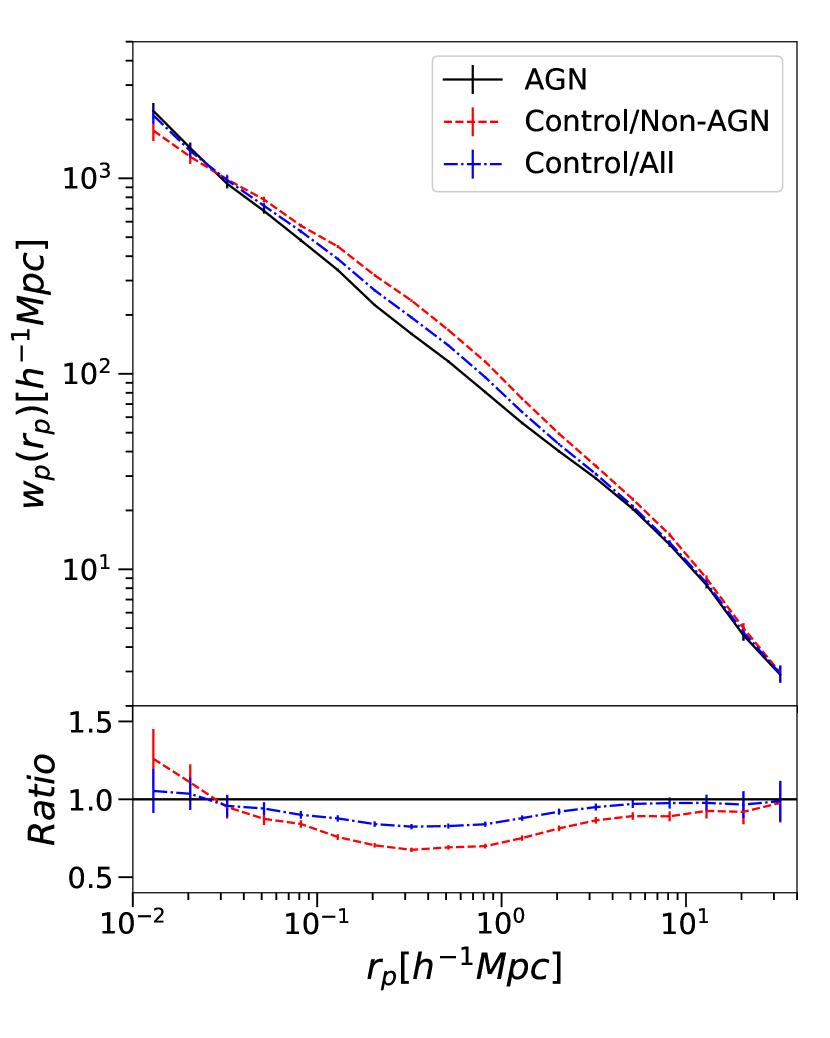
Figure 1: Top: plotted as black crosses connected by the solid line is the projected cross-correlation function $w_{p}(r_{p})$ between the full AGN sample and the reference galaxy sample. The dashed red line and the dotted blue line present the $w_{p}(r_{p})$ with respect to the same reference sample, as measured for two control samples, constructed from the galaxies with no AGN and the full reference sample, respectively. Bottom: ratio of the $w_{p}(r_{p})$ measurement of AGN to that of the control samples. Symbols/lines are the same as in the top panel.

We begin by estimating $w_{p}(r_{p})$ for the full AGN sample and the corresponding control sample of galaxies, both with respect to the reference sample. The measurements are shown in Figure 1. The upper panel displays the amplitudes of the $w_{p}(r_{p})$ as a function of $r_{p}$, with the black line for the AGN sample and the blue dotted line for the control sample. In the lower panel the blue dotted line shows the ratio of the $w_{p}(r_{p})$ between the AGN and the control sample, which is a measure of the scale-dependent bias of the AGN relative to control galaxies of similar properties. The two samples are indistinguishable in clustering amplitude on both large scales with $r_{p}$ above a few Mpc and small scales with $r_{p}$ below a few tens of kpc. At intermediate scales the AGN are clustered less strongly when compared to the control galaxies. This anti-bias is strongest at a few $\times 100h^{-1}$kpc, and becomes weaker when one goes to both larger and smaller scales.

The AGN anti-bias at intermediate scales was originally found in L06. We note that the control samples in that paper were constructed in a slightly different way, in the following two aspects. First, L06 considered only non-AGN, thus excluding the AGN from the control samples. Therefore, the anti-bias discovered in that work was actually the difference between galaxies with an AGN and those without an AGN. Second, as described in Section 2, the control sample used in the current work is closely matched with the AGN sample in five parameters including redshift, stellar mass, concentration, central stellar velocity dispersion and optical color, while L06 considered the first four parameters only. Here we additionally include $g-r$ color, considering the known fact that galaxy clustering depends on color over a wide range of scales even when the stellar mass is limited to a narrow range (e.g. Li et al., 2006a).

For a better comparison with L06, we have also constructed control samples of non-AGN, which are the galaxies from our reference sample that are neither identified as AGN on the BPT diagram, nor selected as low-S/N AGN. We have constructed two control samples of non-AGN: one matched in redshift, stellar mass, concentration and central stellar velocity dispersion, thus in exactly the same way as in L06, and the another matched additionally in $g-r$ as in this work. In Figure 1 we show the $w_{p}(r_{p})$ measurement and the AGN-to-control $w_{p}(r_{p})$ ratio obtained using the non-AGN control sample that is matched in five parameters, as the red dashed line in both panels. The results for the control sample matched in four parameters are very similar, and are not shown in the figure for clarity. The anti-bias is more pronounced when the control sample includes non-AGN only, with a minimum $w_{p}(r_{p})$ ratio of $\sim 0.7$ occurring also at a few $\times 100h^{-1}$kpc. When compared to the result from the control sample of all galaxies, the anti-bias extends to larger scales, with a $w_{p}(r_{p})$ ratio of $\sim 0.9$ even at scales exceeding 10 Mpc. At smallest scales the $w_{p}(r_{p})$ ratio seems to suggest a slightly positive bias, which should not be overemphasized, however, given the large errors at these scales. All these results are in very good agreement with L06 (see their Figure 3).

We conclude that the anti-bias of AGN, as originally reported in Paper I with respect to non-AGN, still exists but becomes weaker when the bias is measured relative to the general population of galaxies regardless of nuclear activity. The weaker anti-bias is naturally expected, since the inclusion of some AGN into the control sample must have lowered the intermediate-scale clustering to some degree, thus reducing the difference between the AGN and the control sample. In what follows we will use the control samples selected from all galaxies, unless otherwise stated.

3.3 Joint dependence on mass, color and $D_{n}(4000)$

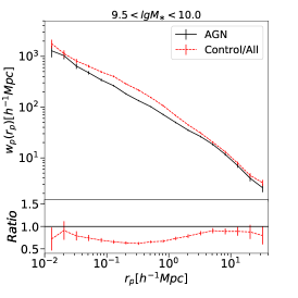
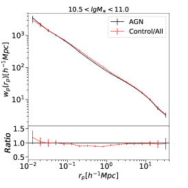
Figure 2: Top: $w_{p}(r_{p})$ in different stellar mass intervals as indicated above each panel, for all AGN (red dashed lines) and for control samples (black solid lines). Bottom: ratio of $w_{p}(r_{p})$ between the AGN and control samples in the top panel.

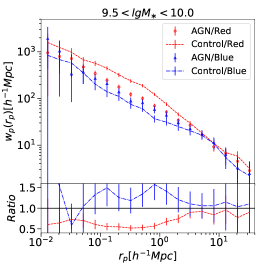
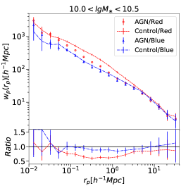
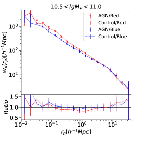
Figure 3: Top: $w_{p}(r_{p})$ in different stellar mass intervals ( indicated above each panel), for AGN hosted by red (red circles) and blue (blue triangles) galaxies, and for the corresponding control samples. Bottom: ratio of $w_{p}(r_{p})$ between the AGN samples and their control samples. Symbols/lines are the same as in the top panel.

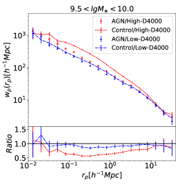
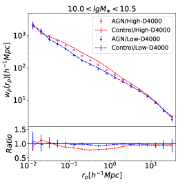
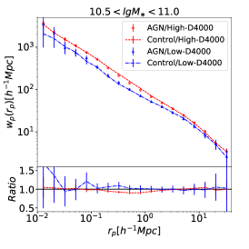
Figure 4: Top: $w_{p}(r_{p})$ in different stellar mass intervals ( indicated above each panel), for AGN hosted by galaxies with high $D_{n}(4000)$ (red circles) and low $D_{n}(4000)$ (blue triangles), and for the corresponding control samples. Bottom: ratio of $w_{p}(r_{p})$ between the AGN samples and their control samples. Symbols/lines are the same as in the top panel.

Galaxy clustering is known to depend on a variety of properties. It is interesting to study how the anti-bias of AGN depends on the properties of their host galaxies. We consider three physical parameters: stellar mass (M_∗), optical color ($g-r$) and the 4000-Å break stength $D_{n}(4000)$. These are the galaxy properties that are most related to environment (e.g. Kauffmann et al., 2004; Blanton & Moustakas, 2009) or clustering (e.g. Li et al., 2006a). The optical color and $D_{n}(4000)$ are similar in the sense that they are indicator of the mean stellar age and recent star formation history of galaxies.

We first divide all the AGN in our sample into three subsamples with different stellar mass intervals: $9.5<$$\log_{10}($M_∗$/$M${}_{\odot})$$<10$, $10<$$\log_{10}($M_∗$/$M${}_{\odot})$$<10.5$, and $10.5<$$\log_{10}($M_∗$/$M${}_{\odot})$$<11$. For each AGN subsample, we construct a control sample by selecting galaxies from the reference sample, closely matched with the AGN sample in the four parameters as described in Section 2. We then estimate $w_{p}(r_{p})$ for the AGN subsamples and the corresponding control samples. The $w_{p}(r_{p})$ measurements are shown in Figure 2. Panels from left to right correspond to the three stellar mass intervals. Panels in the upper row compare the $w_{p}(r_{p})$ measurements for the AGN and control samples, while the lower panels display the AGN-to-control $w_{p}(r_{p})$ ratio.

As can be clearly seen from the figure, the anti-bias is most remarkable for AGN that are hosted by galaxies with lowest stellar masses, becoming less pronounced at higher stellar masses. For the subsample with highest M_∗, the AGN and the control galaxies show almost the same clustering behaviors, and the anti-bias at a few $\times 100h^{-1}$kpc is no longer significantly seen. This result shows that the anti-bias observed previously for the full AGN sample is dominately contributed by the subset of AGN that are hosted by relatively low-mass galaxies.

Next, for each stellar mass subsample, we further divide the AGN into two subsets, with “red” or “blue” color, according to the $g-r$ of their host galaxies. To the end, we have determined a mass-dependent color divider: $(g-r)_{\mbox{cut}}=-1.399+0.2168$$\log_{10}($M_∗$/$M${}_{\odot})$, based on the distribution of the reference sample galaxies on the $\log_{10}($M_∗$/$M${}_{\odot})$ versus $g-r$ plane. We have corrected the sample incompleteness caused by the volume effect of the survey by weighting each galaxy by $1/V_{\mbox{max}}$, where $V_{\mbox{max}}$ is the maximum volume over which the galaxy can be included in our sample. A galaxy is classified as a red galaxy if its $g-r$ is larger than the $(g-r)_{\mbox{cut}}$ at its stellar mass. Otherwise it is a blue galaxy. For each AGN subsample we construct a control sample in the same way as above.

Figure 3 displays the $w_{p}(r_{p})$ measurements for the AGN subsamples selected by M_∗ and color. Panels from left to right are for the three mass intervals. In each panel, results for the AGN in red (blue) hosts and the corresponding control sample are plotted in red (blue) symbols and the dashed-red (dotted-blue) line. We find that, when limited to blue galaxies, the AGN show almost no or very weak anti-bias, and this is true at all scales and for all masses. It is interesting that the anti-bias at intermediate scales is hold only for AGN in red galaxies. This result clearly shows that the overall anti-bias seen for the full AGN sample is dominated by those AGN in low-mass red galaxies, while the AGN hosted by blue galaxies of all masses or red galaxies of high masses are clustered in the same way as the control galaxies.

Finally, we examine the co-dependence of AGN clustering on mass and $D_{n}(4000)$, repeating the above analysis but using $D_{n}(4000)$ instead of $g-r$ to divide galaxies in a given mass range into subsamples of high or low $D_{n}(4000)$. Figure 4 shows the results which are very similar to what is seen from the previous figure on the co-dependence on mass and color. On one hand, there is little difference in $w_{p}(r_{p})$ between the AGN of low $D_{n}(4000)$ and the control galaxies. On the other hand, strong anti-bias is observed for the AGN hosted by galaxies of high $D_{n}(4000)$ and intermediate-to-low masses. The similarity is well expected, because $g-r$ and $D_{n}(4000)$ are both related to the recent star formation history of galaxies, as mentioned above.

A common result from Figures 1-4 is that, on large scales with $r_{p}$ above a few Mpc, the AGN always show the same clustering amplitudes as the control galaxies, and this is true for all the mass intervals and for all the subsets selected by $g-r$ or $D_{n}(4000)$. It is known that the amplitude of clustering at scales larger than a few Mpc is an indicator of the dark matter halo mass of galaxies. Therefore, our finding implies that the AGN and control galaxies, once matched closely in the main properties, intend to populate dark matter halos of similar mass. In addition, we also note from both Figure 3 and Figure 4 that, at fixed stellar mass and at the intermediate scales, the AGN with red colors or high $D_{n}(4000)$ are more clustered than the AGN with blue colors or low $D_{n}(4000)$, although the red or high-$D_{n}(4000)$ AGN are anti-biased at these scales relative to the control sample.

3.4 Dependence on black hole mass, AGN power and AGN type

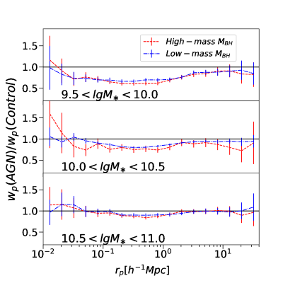
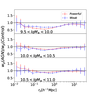
Figure 5: AGN-to-control ratio of $w_{p}(r_{p})$ for galaxies in different stellar mass bins (indicated in each panel), and for AGN with high or low black mass (left panels), or AGN with high or low Eddington ratio (right panels). See the text for details.

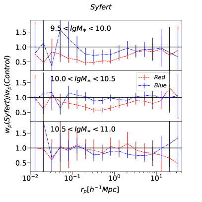
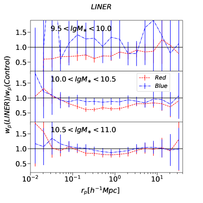
Figure 6: AGN-to-control ratio of $w_{p}(r_{p})$ for different stellar mass bins (indicated in each panel), and for Seyferts (left panels) and LINERs (right panels). In each panel, the red/blue lines are for AGN hosted by galaxies of red/blue colors.

In this subsection we further study the dependence of AGN clustering, particularly the anti-bias at intermediate scales, on the properties of the AGN themselves. As described in Section 2, we have estimated a black hole mass M${}_{\mbox{BH}}$ and the accretion rate relative to the Eddington rate $L$[O iii]/M${}_{\mbox{BH}}$ for each AGN in our sample. For a given stellar mass interval, we divide the AGN into two subsets with either high or low M${}_{\mbox{BH}}$, or with either high or low $L$[O iii]/M${}_{\mbox{BH}}$. We adopt the median values of M${}_{\mbox{BH}}$ and $L$[O iii]/M${}_{\mbox{BH}}$  in a given stellar mass bin as the dividers, so that the two subsets have the same sample size. A control sample is constructed for each subsample in the same way as above. Figure 5 displays the $w_{p}(r_{p})$ ratio between the AGN and control samples. In the left-hand panel, the red and blue lines in each panel are results for the AGN subsamples with high and low M${}_{\mbox{BH}}$, respectively, while the three panels are for the three stellar mass bins. Similarly, the right-hand panel compares the AGN-to-control $w_{p}(r_{p})$ ratio for the “powerful” AGN (high $L$[O iii]/M${}_{\mbox{BH}}$, red line) and the “weak” AGN (low $L$[O iii]/M${}_{\mbox{BH}}$, blue line).

As can be seen from Figure 5, the clustering amplitude shows very weak or no dependence on either M${}_{\mbox{BH}}$ or $L$[O iii]/M${}_{\mbox{BH}}$, and this is true for all stellar masses and at all scales probed. Slight difference is observed in the lowest mass range ($9.5<$$\log_{10}($M_∗$/$M${}_{\odot})$$<10$, the top-right panel), where the powerful AGN appear to show stronger anti-bias than the weak AGN on scales $0.1h^{-1}$Mpc$<r_{p}<1h^{-1}$Mpc. This result is in broad agreement with L06 which found a marginal tendency for powerful AGN to be more strongly anti-biased than weak AGN at the highest Eddington ratios. L06 also found the anti-bias to slightly depend on black hole mass with more massive black boles showing stronger anti-bias. This effect may be attributed to the different way of constructing control samples as we point out above. However, the dependence on black hole mass was rather weak and wasn’t of high significance due to the large error bars.

In Figure 6 we examine the co-dependence of clustering on mass and color but separately for Seyferts (left panel) and LINERs (right panel). In each case we show the AGN-to-control $w_{p}(r_{p})$ ratios, compared for red and blue galaxies for a given stellar mass range. Although the measurements become noisy due to smaller sample sizes when compared to the measurements in previous figures, the $w_{p}(r_{p})$ ratios of both Seyferts and LINERs depend on mass and color in exactly the same way as the $w_{p}(r_{p})$ ratios of the whole AGN sample. The intermediate-scale anti-bias is observed only for Seyferts/LINERs hosted by low-mass red galaxies, and there is no effect for blue galaxies or red galaxies of high masses. This finding shows that the anti-bias at intermediate scales and its co-dependence on mass and color are a general property of different types of AGN.

4 Central fractions and halo properties based on the SDSS group catalog

In L06, the antibias observed for the full AGN sample was interpreted by a higher fraction of central galaxies in the AGN sample than the control sample. A simple halo-based model in which the central fraction of AGN ($f_{c}$) is the only free parameter could well reproduce the $w_{p}(r_{p})$ measurement of both AGN and control galaxies. In this section we make use of the SDSS galaxy group catalogue (see §2.3) to estimate $f_{c}$ for both the AGN samples and the control samples, as a function of galaxy mass and color. In addition, we also examine the dark matter halo mass and assembly history (indicated by the stellar mass gap between the most massive and the second most massive galaxy in a group), using the same group catalogue. These parameters are known to be correlated with clustering at different scales.

4.1 Central fraction of AGN as a function of stellar mass and color

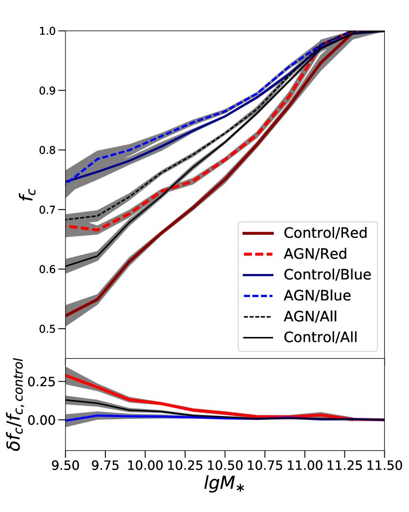
Figure 7: Top: central fraction $f_{c}$ is plotted as a function of stellar mass for all AGN (black dashed line), and for AGN hosted by red (red dashed line) and blue (blue dashed line) galaxies, compared to the $f_{c}$ of the corresponding control samples (black/red/blue solid lines). Bottom: relative difference of $f_{c}$ between AGN and control samples. Lines are the same as in the top panel. In both panels, the lines are the median $f_{c}$ in given sample, and the shaded regions indicate the 1$\sigma$ scatter around the median.

We aim to estimate the central fraction for AGN/control samples with both red and blue colors, and in different stellar mass bins. For this purpose, we have selected a set of four volume-limited samples on the plane of $\log_{10}(M_{\ast})$ versus redshift out of the reference sample, adopting the mass thresholds and redshift intervals as in von der Linden et al. (2010) (see their Fig.5). The selection criteria ensure that, for each of the four samples, both the red and blue populations are complete down to the chosen mass threshold and within the corresponding redshift range. We then match the samples with the SDSS group catalog to obtain their central/satellite classification and dark matter halo properties.

Figure 7 shows $f_{c}$ as a function of $\log_{10}(M_{\ast})$ for the full AGN sample and the AGN hosted by red and blue galaxies. Results of the corresponding control samples are also plotted for comparison. The relative difference of $f_{c}$ between the AGN to control samples are plotted in the smaller panel of the same figure. Overall, $f_{c}$ increases with increasing stellar mass in all the cases, reaching $100\%$ at the highest masses ($\log_{10}M_{\ast}>11.25$). At lower masses, $f_{c}$ at fixed mass differ from sample to sample, but basically the blue populations including both AGN and control galaxies have higher $f_{c}$ when compared to the red populations at the same mass.

Comparing the AGN and control samples, we find the $f_{c}$ of the full AGN sample to be higher than that of the control sample at stellar masses below $\sim 10^{10.5}M_{\odot}$. The relative difference is largest at lowest masses, $\sim 13\%$ at $\log_{10}M_{\ast}\sim 9.5$, and decreases with mass. At masses above $\sim 10^{10.5}M_{\odot}$ the AGN and control samples present the same central fractions. More interestingly, when the AGN are divided into subsets with red and blue colors, we find the same mass-dependent differences to be hold in the red samples, and the AGN and control galaxies of blue colors present very similar $f_{c}$ at all masses. We note that consistent results were found in an earlier paper by Pasquali et al. (2009).

4.2 Halo properties of AGN according to central/satellite division

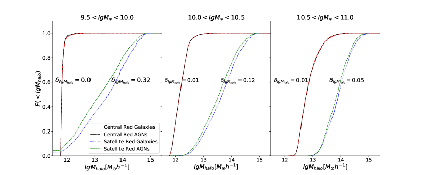
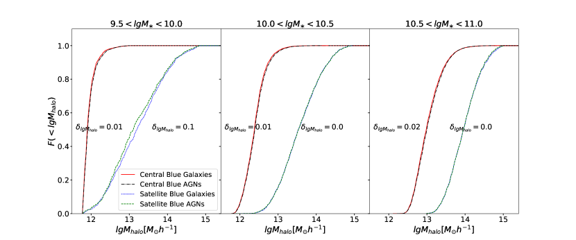
Figure 8: Cumulative fractions of dark halo mass are plotted for AGN (dashed lines) and control galaxies (solid lines), in different stellar mass bins (indicated above each panel) and for red (upper panels) and blue (lower panels) colors. The difference in the median value of $\log_{10}(M_{halo})$ between each AGN sample and the corresponding control sample is indicated.

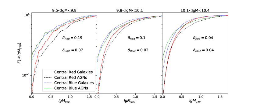
Figure 9: Cumulative fractions of stellar mass gap of galaxy groups, $\log_{10}M_{gap}$, are plotted for AGN (dashed lines) and control galaxies (solid lines), in different stellar mass bins (indicated above each panel) and for red (black/red) and blue (blue/green) colors. The difference in the median value of $\log_{10}M_{gap}$ between each AGN sample and the corresponding control sample is indicated.

In Figure 8 we compare the cumulative distribution of the halo mass for the AGN and control samples in different mass bins, but for central and satellite galaxies separately. For this plot we have taken the halo mass estimates, as well as the central/satellite classification from the SDSS group catalogue. The upper to lower panels present results for AGN in red and blue galaxies, respectively. Panels from left to right correspond to different stellar mass bins. The AGN and control galaxies show identical halo mass distributions in all cases regardless of color, if they are central galaxies of their halos. In case of satellite galaxies, in contrast, AGN are found in less massive halos than control galaxies, and the effect is seen mainly for the red populations and is stronger at lower masses.

In fact, the lower halo mass of the AGN samples of red colors can be seen from Figs 3 and 4. For the samples with red colors (or low-$D_{n}(4000)$) and lowest stellar masses, the AGN antibias is detected out to $\sim 10$Mpc, much larger than the scale of 1-3Mpc in other cases. The clustering amplitude on scales larger than a few Mpc is known to be an indicator of dark halo mass. The weaker clustering at large scales thus implies that the AGN in the low-mass red galaxies are hosted by less massive halos, compared to the control sample, although the two samples are already closely matched in many parameters that are known to be correlated with large-scale clustering. Apparently the clustering measurements and the halo mass distributions from the group catalog agree very well with each other.

In Figure 9 we compare the stellar mass gap of the host groups between our AGN and control samples. The stellar mass gap for a given group, $\log_{10}M_{gap}$, is defined by the difference in $\log_{10}M_{\ast}$ between the most massive galaxy (equivalently the central galaxy) and the second most massive galaxy (the most massive satellite galaxy). In this plot we only consider AGN and control galaxies that are classified as central galaxies of their groups. In addition, we restrict ourselves to stellar mass below $10^{10.4}M_{\odot}$, because the AGN and control galaxies at higher stellar masses show identical distributions in this parameter. As can be seen from the figure, in the case of blue colors, AGN and control galaxies at given mass tend to have very similar distributions of $\log_{10}M_{gap}$. Differences between AGN and control galaxies are seen in the case of red colors and at stellar mass below $\sim 10^{10}M_{\odot}$ (the left two panels), where the host groups of AGN tend to have a larger stellar mass gap than the host groups of contral galaxies.

Previous studies have suggested that the luminosity or stellar mass gap defined this way may be a good tracer of the assembly history of dark matter halos, and that galaxy groups with a large luminosity gaps are believed to form earlier than galaxy group with a small luminosity gap (e.g. Dariush et al., 2007, 2010). A large luminosity or stellar mass gap has thus been adopted as one of the observational criteria for identifying “fossil groups” (e.g. Jones et al., 2003; Dariush et al., 2007, 2010; Tavasoli et al., 2011; Hess et al., 2012). On the other hand, it has been known for more than a decade that, the clustering of dark halos is not purely determined by their mass, but also related to their assembly history (e.g. Gao et al., 2005; Gao & White, 2007). Therefore, the larger stellar mass gap for the AGN host groups may be suggesting that AGN prefer to occur in early-formed dark matter halos.

5 Halo-based modeling of the mass and color dependence of AGN clustering

In this section we attempt to interpret the co-dependence of AGN clustering on the stellar mass and color of host galaxies, in the context of halo occupation models. The clustering difference between AGN and control samples are seen only at scales between about 100kpc and 1-3 Mpc, where the AGN are more weakly clustered than the control galaxies with the same mass, color and structural properties. On larger scales, the AGN and control galaxies present similar clustering amplitudes, indicating that they are hosted by halos of similar dark matter mass. At intermediate scales, as shown in L06, the antibias observed for the full AGN sample can be simply interpreted if AGN are preferentially found in central galaxies, which are located at the center of dark matter halos. This simple model was able to successfully reproduce the projected 2PCF for both the AGN and the control sample of non-AGN, if a central fraction of 84% and 73% were adopted for the two samples respectively.

In § 3, we showed that the antibias discovered in L06 is essentially dominated by a subset of AGN that are hosted by low-mass red galaxies, while the AGN in galaxies of blue colors or high masses present similar clustering properties to control galaxies. Previous studies of halo occupation models for galaxy samples selected by mass (or luminosity) and color have shown that the halo occupations depend strongly on these two properties (e.g. Zehavi et al., 2011). Therefore, the mass and color dependence of galaxy clustering must be considered in any halo-based models before one can further model the clustering of AGN. In the rest of this section, we will first apply two commonly-applied halo models, the subhalo abundance matching model (SHAM) and the subhalo age distribution matching model (SADM), to assign a stellar mass and a color to each model galaxy in our simulation. We will then select AGN from the model galaxies by applying a simliar model to that proposed in L06, which assumes AGN to be preferentially found at the center of dark halos.

5.1 Subhalo abundance matching and subhalo age distribution matching

Our models are constructed based on the Millennium Simulation (see § 2.5), for which dark matter halos and subhalos at different snapshots are identified, and halo merger trees are constructed describing the growth history of the halos. We take all the subhalos at $z=0$, and assign a stellar mass to each subhalo by applying the subhalo abundance matching model (SHAM). This model has been widely applied for linking galaxies of different stellar masses to halos of different dark matter masses (Vale & Ostriker, 2004; Conroy et al., 2006; Shankar et al., 2006; Conroy et al., 2007; Baldry et al., 2008; Moster et al., 2010; Guo et al., 2010; Neistein et al., 2011b, a; Yang et al., 2012; Li et al., 2012). In this model each (sub)halo is assumed to host a galaxy, of which the stellar mass is an increasing function of the maximum mass ever attained by its halo. In practice, the relationship between dark matter halo mass $M_{200}$ and galaxy stellar mass $M_{\ast}$ is obtained simply by matching the number density of halos with mass above $M_{200}$ with the number density of galaxies with stellar mass above $M_{\ast}$. To the end, we have used the stellar mass function of galaxies in the local Universe estimated by Li & White (2009) from the SDSS/DR7 galaxy sample, which is updated in Guo et al. (2010) using the SDSS “model” magnitudes instead of “Petrosian” magnitudes.

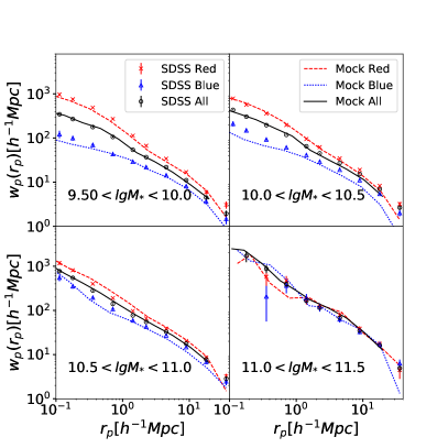
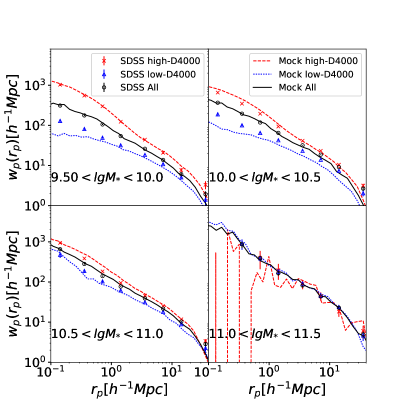
Figure 10: Comparison of projected auto-correlation function of all galaxies in the SDSS (symbols) and in our model (lines). Different panels are for different stellar mass bins, as indicated. In each panel, the red and blue points/lines represent red and blue galaxies, while the black points/line represent all the galaxies in the given mass range.

For each model galaxy, we then further assign a color or a $D_{n}(4000)$ by applying the subhalo age distribution model (SADM), as recently presented by Hearin & Watson (2013). Following these authors, we define a redshift $z_{starve}$ for each model galaxy by

$$z_{starve}=\max(z_{form},z_{acc},z_{char}),$$ (3)

where $z_{form}$ is the halo formation time at which the dark matter halo transitions from the fast-accretion regime to the slow-accretion regime (Wechsler et al., 2002), $z_{acc}$ the epoch when the galaxy was last the central galaxy of its own halo, and $z_{char}$ is the epoch when the halo mass exceeds $10^{11.5}M_{\ast}h^{-1}$. We note that the mass threshold adopted here for defining $z_{char}$ is slightly lower than the value suggested in (Hearin & Watson, 2013), $10^{12}M_{\ast}h^{-1}$, as the new mass threshold allows our model to better reproduce the observed color dependence of galaxy clustering in this work. As discussed in (Hearin & Watson, 2013), the $z_{starve}$ defined this way is expected to encompass physical characteristics of halo mass assembly that may be responsible for quenching the star formation in the galaxy, thus a driving parameter for its color or mean stellar age. At fixed stellar mass, galaxy color is assumed to be an increasing function of $z_{starve}$, and so can be determined by matching the observed color distribution of galaxies at the given stellar mass with the $z_{starve}$ distribution of dark halos corresponding to the same stellar mass.

Applications of the SHAM and SADM models to the Millennium Simulation results in a complete mock catalog of model galaxies at $z=0$, each assigned both a stellar mass $M_{\ast}$ and an optical color $g-r$ (or a $D_{n}(4000)$). In Figure 10, we compare the projected 2PCF $w_{p}(r_{p})$ as measured for the reference galaxy sample and the model galaxy catalog, for different stellar mass intervals and for subsets of galaxies with red/blue colors (upper panels), or high-/low-$D_{n}(4000)$ (lower panels) at fixed mass. We adopt a mass-dependent color divider to divide galaxies into red and blue subsets, $g-r=-1.399+0.2168\times\log_{10}M_{\ast}$, determined by fitting a double Gaussian profile to the distribution of $g-r$ at fixed $M_{\ast}$ following the method described in Li et al. (2006a). A mass-dependent divider of $D_{n}(4000)$ is determined in the same way and applied to divide galaxies at fixed mass into subsets of high- and low-$D_{n}(4000)$.

The figure shows that, as expected, the co-dependence of galaxy clustering on stellar mass and optical color (or $D_{n}(4000)$) can be well reproduced with the model, particularly for the red galaxies (or those with higher $D_{n}(4000)$) and for the galaxies as a whole. For blue galaxies or galaxies of low-$D_{n}(4000)$, the model works well at all masses except the interval of $10<\log_{10}(M_{\ast}/M_{\odot})<10.5$, where the model predicts weaker clustering at all the scales probed. A similar discrepancy is also observed in Hearin & Watson (2013), where the model underpredicts the clustering on scales above $\sim 1$Mpc for the blue galaxies with $r$-band absolute magnitudes in the range $-20<M_{r}<-21$, which is roughly corresponding to the mass range mentioned above, according to the $r$-band luminosity function and stellar mass function of SDSS galaxies (e.g. Blanton et al., 2003b; Li & White, 2009). We note that, in the lowest-mass bin ($9.5<\log_{10}(M_{\ast}/M_{\odot})<10$), the clustering of blue galaxies and those with low $D_{n}(4000)$ in the model is also slightly lower than the observation for scales smaller than $\sim 1$Mpc. Despite these slight discrepancies, overall the model is in good agreement with the data, and thus forms a good basis for us to further model the dependence of AGN clustering on galaxy mass and color. We will keep these discrepancies in mind when modelling the AGN clustering in the rest of the paper, though. Given the highly similar results for $(g-r)$ and $D_{n}(4000)$, as seen in both the previous section and the current one, we will concentrate on $(g-r)$ in what follows. We note that we have done the same analysis for $D_{n}(4000)$, finding very similar results to $(g-r)$.

5.2 Modelling the AGN clustering with the simple model of L06

The mass and color dependence of the central fractions are well expected by the simple model of L06, in which $f_{c}$ is the driving parameter for the antibias of AGN relative to the control sample. In the previous section we have shown that the antibias is observed only for the AGN in red galaxies with masses below $\sim 10^{10.5}M_{\odot}$. Therefore, it is natural to expect that the same model as proposed in L06 will well explain the $w_{p}(r_{p})$ measurements for the samples of different masses and colors as measured in this work. We apply the model of L06 to select AGN from the model galaxy catalog constructed above, according to the mass-dependent central fraction of AGN and control galaxies, but for red and blue colors separately. We divide the model galaxies into red and blue populations according to the $(g-r)$, in the same was as done for the real sample. For a selected sample of model AGN, we construct a control sample by requiring it closely match the model AGN sample in both stellar mass and color. We don’t consider other parameters such as concentration and stellar velocity dispersion which are not available in our current model, but we argue that the dependence of clustering on those parameters are known to be much weaker than the dependence on mass and color.

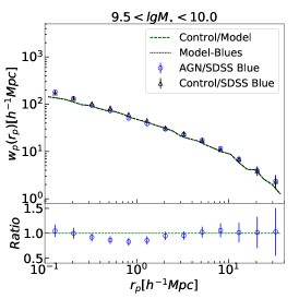
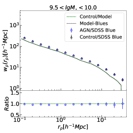
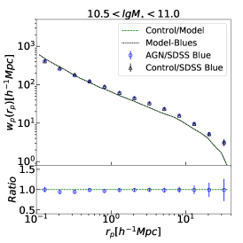
Figure 11: Top: open circles and triangles show the $w_{p}(r_{p})$ for AGN and control galaxies with blue colors, while the green dashed and black dotted lines show the results for the corresponding control samples. Different panels are for different stellar mass bins as indcated. Bottom: ratio of $w_{p}(r_{p})$ between AGN and control galaxies. Symbols/lines are the same as in the top panel.

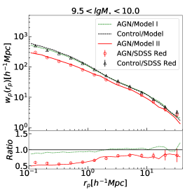
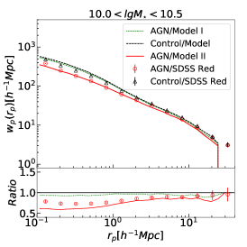
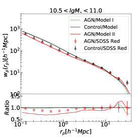
Figure 12: Top: open circles and triangles show the $w_{p}(r_{p})$ for AGN and control galaxies with red colors. The three lines are the results for the models. The blue dashed line for the control galaxies in the models, while the green dotted and solid red lines are for the AGN in the two models separately (see the text for details. Bottom: ratio of $w_{p}(r_{p})$ between AGN and control galaxies. Symbols/lines are the same as in the top panel.

For the AGN/controls of blue colors, since AGN and control galaxies present similar central fractions at fixed mass, we simply select a random subset of blue galaxies to be our model AGN, thus essentially assuming AGN are found equally in every galaxy if its color is blue. Figure 11 compares the $w_{p}(r_{p})$ predicted by this model with the observation, for the three stellar mass intervals. As expected, the AGN and control galaxies in the model show identifical clustering properties at given mass, which well match the $w_{p}(r_{p})$ of the SDSS AGN and control samples. We note that the model slightly underpredicts the clustering amplitude at scales above a few Mpc for the two high-mass bins, which is the problem of the model of the blue galaxy population as pointed out in the previous subsection. For AGN in blue galaxies, it is clear that they show no preference in terms of halo mass and environment of all scales, when compared to control galaxies of the same mass and color.

For the AGN/controls of red colors, we select AGN from the red galaxies in the model catalog, requiring the relative difference of $f_{c}$ between the AGN and control sample to follow the observation (see Figure 7), which can be described by

$$\delta_{f_{c}}/f_{c,control}=0.1434\times(\log_{10}M_{\ast})^{2}-3.1092\times\log_{10}M_{\ast}+16.8724.$$ (4)

The $w_{p}(r_{p})$ predicted by this model are compared to the observation in Figure 12, again for the three mass intervals separately. In the figure, the green dotted lines are for the AGN in the model, while the black dashed lines are for the control samples of model galaxies. The green dotted lines in the smaller panels present the AGN-to-control ratio of $w_{p}(r_{p})$ for the model. To our surprise, the AGN and control galaxies in the model show similar clustering amplitudes on all scales and at all masses, with no significant antibias everywhere. The model indeed predicts slightly weaker clustering on scales below a few Mpc for AGN in the two low-mass bins, but the difference is much less significant than the observed antibias.

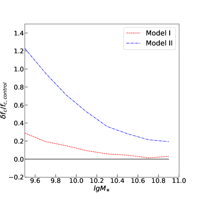
Figure 13: Fraction of AGN in central galaxies as a function of stellar mass, as adopted by the two models separately. See the text for details.

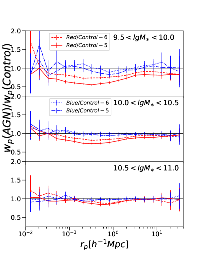
Figure 14: AGN-to-control ratio of $w_{p}(r_{p})$ for different stellar mass bins (indicated in each panel), and for AGN in red (red lines) and blue (blue lines) galaxies separately. In each panel, the dotted lines are for the AGN and control samples matched in five parameters, while the dashed lines for the samples matched additionally in central fraction.

L06 has shown that a higher central fraction for AGN can make the model reproduce the observed antibias at scales between $\sim 100$kpc and a few Mpc. In that work, however, the central fraction was assumed to be a free parameter and constrained purely by the clustering measurements. It is interesting to see whether the model can still work if $f_{c}$ is a free parameter. In this case, $f_{c}$ for AGN in a given mass bin is determined by fitting the $w_{p}(r_{p})$ of the model to the observed one. The clustering measurements of the AGN sample in the best-fit model are shown also in Figure 12, but in solid red lines. Results of the control samples remain unchanged, and so are not plotted. As can be seen, the model can truely reproduce both the $w_{p}(r_{p})$ measurements and the AGN-to-control antibias at scales below a few Mpc, although the antibias in the model appears to be even stronger. For convenience, in what follows we will call this model as Model II and the model which adopts the observed $f_{c}$ as Model I.

In Figure 13 we plot $f_{c}$ as a function of stellar mass for both Model II (the blue dotted line) and Model I (the red dashed line). The central fractions of AGN in Model II are higher by a factor of $\sim$4 than the fractions estimated from the SDSS group catalog. We should point out that, for simplicity, the fitting for Model II is done for the three mass bins simultaneously, by multiplying both sides of Eqn. (4) by a common factor. We can well expect the model to better match the data in the two high-mass bins if the fitting is done for the different mass bins independently. Our purpose here is not to obtain an accurate model. Rather, we aim at demonstrating that the central fraction alone is able to explain the observed mass-dependence of the AGN antibias, and our result here shows this is indeed the case.

On the other hand, however, the fact that the model requires central fractions much higher than the real sample implies that the observed antibias of AGN cannot be purely explained by a higher $f_{c}$. To test this out, we have done an additional analysis of the real sample, in which we further require each control sample to have the same central fraction as the corresponding AGN sample. Results of this analysis are shown in Figure 14, where we plot the AGN-to-control $w_{p}(r_{p})$ ratio as a function of $r_{p}$. The three panels are for the different mass intervals, and in each panel the red/blue lines are for the red and blue subsamples respectively. The results of the new analysis are shown in dashed lines, and the results from the previous section where the control samples are not matched in central fraction are shown in dotted lines, for comparison. Generally, the AGN antibias becomes weaker, but is still significantly detected, as can be seen in the low-mass red subsamples. This result clearly demonstrates that the central fraction can partly but not entirely explain the AGN antibias.

6 Summary and Conclusions

We have studied the joint dependence of AGN clustering on galaxy stellar mass and color (or $D_{n}(4000)$), using a sample of $\sim 10^{5}$ narrow-line AGN and a sample of about half a million reference galaxies, both selected from the final data release of the Sloan Digital Sky Survey (SDSS/DR7 Abazajian et al., 2009). The AGN are divided into different stellar mass bins, and for a given mass bin they are further divided into red and blue subsamples according to the optical color $(g-r)$ or $D_{n}(4000)$ of their host galaxies. For each AGN sample, we have constructed a control sample from all the reference galaxies which are closely matched with the AGN sample in redshift, stellar mass, color, stellar velocity dispersion and concentration index. For both the AGN sample and its corresponding control sample, we then estimate the projected cross-correlation function $w_{p}(r_{p})$ with respect to the reference galaxy sample, and compare the $w_{p}(r_{p})$ measurements between AGN and control galaxies. Next, we make use of the SDSS/DR7 galaxy group catalogue constructed by Yang et al. (2007) to further examine the halo properties of the AGN and control galaxies, but for the AGN/controls in central and satellite galaxies separately. We consider three properties of the host groups: the fraction of central galaxies in the sample ($f_{c}$), the halo mass distribution, and the stellar mass gap between the two most massive galaxies of a given group. Finally, we apply the commonly-adopted subhalo abundance matching model and subhalo age distribution matching model to populate the (sub)halos in the Millennium Simulation with galaxies of different stellar masses and colors, from which we further select AGN by applying the simple model of Li et al. (2006b) (L06) which assumes AGN to be found more preferentially at the center of dark matter halos.

We have reproduced the AGN antibias as originally found in L06, that is, at scales between about 100kpc and a few Mpc the AGN as a whole are more weakly clustered than the carefully-matched control sample. When we divide the AGN and control galaxies into subsamples by stellar mass and color (or $D_{n}(4000)$), we obtain the following results.

• The antibias previously observed from the full AGN sample is hold only when the AGN host galaxies are less massive than $M_{\ast}\sim 10^{10.5}M_{\odot}$ and have red colors (or high $D_{n}(4000)$), while AGN hosted by red galaxies of higher masses or blue galaxies of all masses show almost identical clustering properties to the control galaxies at all scales. This result is shown to be independent of black hole mass, AGN power and AGN type.

• AGN in blue galaxies are found to have similar mass-dependent central galaxy fraction to the control galaxies. The AGN and control galaxies in this case also show similar halo mass distributions, and this is true even when the central AGN and satellite AGN are considered separately.

• AGN in red galaxies have higher central fraction than the control galaxies, with larger difference at lower stellar masses. On average, the host groups of the AGN associated with red satellite galaxies appear to have lower-than-average dark matter masses, while the host groups of the AGN associated with red central galaxies tend to have larger stellar mass gap, indicative of earlier formation time of their dark halos.

• A simple halo-based model in which the AGN are preferentially found in central galaxies can in principle reproduce the mass and color dependence of the AGN clustering in the SDSS sample. However, the central fraction of AGN in the best-fit model is a factor of $\sim$4 higher than the central fraction of the real AGN sample, implying that the central fraction alone cannot fully explain the AGN clustering properties.

The strong mass and color dependence of the AGN clustering is striking. If hosted in blue galaxies, the AGN show the same clustering and the same group/halo properties as the control galaxies of similar mass, color and structural parameters. The same conclusion is also true for AGN in massive galaxies with $M_{\ast}\ga 10^{10.5}M_{\odot}$. In other words, the AGN activity in blue galaxies or massive galaxies is regulated only by the physical processes internal to galaxies, with no correlations with environment on scales larger than the size of individual galaxies. Previous studies of optically-selected AGN have well established that more than a half of the AGN population in the local Universe are found in massive galaxies with stellar mass above $10^{10.5}M_{\odot}$ (e.g. Heckman, 1980; Ho et al., 1997; Kauffmann et al., 2003a; Hao et al., 2005). Therefore, the majority of the AGN activity in the local Universe is not driven by environmental effects.

The unbiased clustering of AGN in blue galaxies is also a very interesting result. Studies of the correlation of local black hole growth with host galaxy properties have demonstrated that black holes grow more rapidly in galaxies with younger stellar populations (Kauffmann et al., 2003a; Cid Fernandes et al., 2004). Furthermore, Kauffmann & Heckman (2009) have revealed two distinct regimes of black hole growth in low-redshift galaxies, which are strongly linked to the star formation history of the central stellar population of the host galaxies. In one regime, where the host galaxies are undergoing significant central star formation, the distribution of the Eddington ratio ($L_{AGN}/_{Edd}$) universally follows a log-normal form, which is independent of both the black hole mass and current star formation rate. In the other regime, where the host galaxies have little or no ongoing star formation in the central region, the Eddington ratio presents a power-law distribution with a normalization depending on the age of the stellar population. In a more recent work, Aird et al. (2018) used NIR and X-ray deep imaging to measure the probability distribution function of AGN accretion rates as a function of stellar mass for both star-forming and quiescent galaxy populations. The authors also identified two different modes of black hole growth in the two types of galaxies, although their distribution functions of star-forming galaxies are broader than the lognomal distribution as originally identified by Kauffmann & Heckman (2009) and agree better with the Schechter function proposed by Jones et al. (2016). Although it is not immediately clear whether and how the dichotomy in black hole growth is related to the color-dependent AGN clustering, the two observational results are interestingly similar in several aspects, e.g. the universal growth law of black holes with young stellar populations versus the unbiased clustering of AGN with blue colors or low $D_{n}(4000)$, and the non-universal growth law of black holes with old stellar populations versus the antibias of AGN with red colors or high $D_{n}(4000)$. In future works it would be interesting to explore possible physical reasons behind this similarity.

The SDSS group catalog has confirmed the conjecture in L06 that AGN are found preferentially in central galaxies, and the simple halo-based model proposed in the same paper can in principle reproduce the mass and color dependence of the AGN clustering, as shown in this paper. However, the best-fit model requires a central fraction which is substantially too high when compared to the central fraction of the AGN in the group catalog. This demonstrates that, in addition to the central fraction, one would need additional factors in order to have a complete understanding of the AGN clustering. The group catalogue provides some clues as we discussed. First, the AGN in red satellites tend to have lower dark matter halo mass which lead to a weaker clustering amplitude at scales larger than a few Mpc. Second, the groups hosting the AGN of red central galaxies tend to form earlier than the groups hosting the control galaxies of the same mass, color and structural parameters. This implies that the assembly history of the host dark halos should play some role in triggering the AGN activity.

In a recent study of radio-loud AGN in fossil groups of galaxies, Hess et al. (2012) found that two thirds of the 30 fossil group candidates contain a radio-loud AGN at the center of their dominant elliptical galaxy, which is a large fraction as fossil groups were believed to be old, quiescently evolving galaxy systems. These authors argued that the radio luminosity is related to the properties of the group/cluster environment, as well as the mass assembly of the dominant ellipgical galaxy. Obviously our finding above is well consistent with their work. In fact, the fact that radio galaxies prefer to reside at the center of elliptically dominant groups have been noticed in earlier studies (e.g. Best, 2004; Croston et al., 2005). These studies suggested that current AGN activity in fossil groups is linked to the heating of their intergalactic medium (IGM). On the other hand, however, some authors suggested that galaxies with red colors or old stellar populations may have a reservoir of cold gas which can also fuel the central black hole (e.g. Kauffmann et al., 2007; von der Linden et al., 2010). The centers of groups/clusters could well be a preferred environment for these galaxies for the high cooling efficiency and cold gas density in the halo center.

More studies, both theoretical and observational, are needed in order to better understand the role of halo assembly history in driving the AGN activity. Possible ways to go include improving the simple halo model of L06 by considering the halo formation time as an additional parameter to the central fraction, and examining the current hydrodymatical simulations of galaxy formation with different recipes on AGN feedback effects. In addition, next-generation large spectroscopic surveys of high-redshift galaxies to be carried out in the next few years will allow us to extend the study of AGN clustering to redshifts $z>1$. It would be interesting to see whether the mass- and color-dependent AGN clustering is already at place at $z\ga 1$, an epoch at which the cosmic density of both black hole accretion rate and star formation rate are peaked.

References

- Abazajian et al. (2009) Abazajian, K. N., Adelman-McCarthy, J. K., Agüeros, M. A., Allam, S. S., Allende Prieto, C., An, D., Anderson, K. S. J., Anderson, S. F., & et al. 2009, ApJS, 182, 543
- Aird et al. (2018) Aird, J., Coil, A. L., & Georgakakis, A. 2018, MNRAS, 474, 1225
- Allevato et al. (2016) Allevato, V., Civano, F., Finoguenov, A., Marchesi, S., Zamorani, G., Hasinger, G., Salvato, M., Miyaji, T., & et al. 2016, ArXiv e-prints
- Allevato et al. (2014a) Allevato, V., Finoguenov, A., & Cappelluti, N. 2014a, ApJ, 797, 96
- Allevato et al. (2014b) Allevato, V., Finoguenov, A., Civano, F., Cappelluti, N., Shankar, F., Miyaji, T., Hasinger, G., Gilli, R., & et al. 2014b, ApJ, 796, 4
- Baldry et al. (2008) Baldry, I. K., Glazebrook, K., & Driver, S. P. 2008, MNRAS, 388, 945
- Baldwin et al. (1981) Baldwin, J. A., Phillips, M. M., & Terlevich, R. 1981, PASP, 93, 5
- Ballantyne (2017) Ballantyne, D. R. 2017, MNRAS, 464, 626
- Balogh et al. (1999) Balogh, M. L., Morris, S. L., Yee, H. K. C., Carlberg, R. G., & Ellingson, E. 1999, ApJ, 527, 54
- Barrow et al. (1984) Barrow, J. D., Bhavsar, S. P., & Sonoda, D. H. 1984, MNRAS, 210, 19P
- Basilakos (2001) Basilakos, S. 2001, MNRAS, 326, 203
- Basilakos & Plionis (2010) Basilakos, S. & Plionis, M. 2010, ApJ, 714, L185
- Best (2004) Best, P. N. 2004, MNRAS, 351, 70
- Blanton et al. (2003a) Blanton, M. R., Brinkmann, J., Csabai, I., Doi, M., Eisenstein, D., Fukugita, M., Gunn, J. E., Hogg, D. W., & et al. 2003a, AJ, 125, 2348
- Blanton et al. (2003b) Blanton, M. R., Hogg, D. W., Bahcall, N. A., Brinkmann, J., Britton, M., Connolly, A. J., Csabai, I., Fukugita, M., Loveday, J., Meiksin, A., Munn, J. A., Nichol, R. C., Okamura, S., Quinn, T., Schneider, D. P., Shimasaku, K., Strauss, M. A., Tegmark, M., Vogeley, M. S., & Weinberg, D. H. 2003b, ApJ, 592, 819
- Blanton & Moustakas (2009) Blanton, M. R. & Moustakas, J. 2009, ARA&A, 47, 159
- Blanton & Roweis (2007) Blanton, M. R. & Roweis, S. 2007, AJ, 133, 734
- Blanton et al. (2005) Blanton, M. R., Schlegel, D. J., Strauss, M. A., Brinkmann, J., Finkbeiner, D., Fukugita, M., Gunn, J. E., Hogg, D. W., & et al. 2005, AJ, 129, 2562
- Brinchmann et al. (2004) Brinchmann, J., Charlot, S., White, S. D. M., Tremonti, C., Kauffmann, G., Heckman, T., & Brinkmann, J. 2004, MNRAS, 351, 1151
- Cappelluti et al. (2010) Cappelluti, N., Ajello, M., Burlon, D., Krumpe, M., Miyaji, T., Bonoli, S., & Greiner, J. 2010, ApJ, 716, L209
- Carrera et al. (1998) Carrera, F. J., Barcons, X., Fabian, A. C., Hasinger, G., Mason, K. O., McMahon, R. G., Mittaz, J. P. D., & Page, M. J. 1998, MNRAS, 299, 229
- Chabrier (2003) Chabrier, G. 2003, PASP, 115, 763
- Chehade et al. (2016) Chehade, B., Shanks, T., Findlay, J., et al. 2016, MNRAS, 459, 1179
- Cid Fernandes et al. (2004) Cid Fernandes, R., Gu, Q., Melnick, J., Terlevich, E., Terlevich, R., Kunth, D., Rodrigues Lacerda, R., & Joguet, B. 2004, MNRAS, 355, 273
- Coil et al. (2009) Coil, A. L., Georgakakis, A., Newman, J. A., Cooper, M. C., Croton, D., Davis, M., Koo, D. C., Laird, E. S., & et al. 2009, ApJ, 701, 1484
- Coil et al. (2007) Coil, A. L., Hennawi, J. F., Newman, J. A., Cooper, M. C., & Davis, M. 2007, ApJ, 654, 115
- Colless et al. (2001) Colless, M., Dalton, G., Maddox, S., et al. 2001, MNRAS, 328, 1039
- Conroy et al. (2006) Conroy, C., Wechsler, R. H., & Kravtsov, A. V. 2006, ApJ, 647, 201
- Conroy et al. (2007) —. 2007, ApJ, 668, 826
- Constantin & Vogeley (2006) Constantin, A. & Vogeley, M. S. 2006, ApJ, 650, 727
- Croom et al. (2005) Croom, S. M., Boyle, B. J., Shanks, T., Smith, R. J., Miller, L., Outram, P. J., Loaring, N. S., Hoyle, F., & et al. 2005, MNRAS, 356, 415
- Croston et al. (2005) Croston, J. H., Hardcastle, M. J., & Birkinshaw, M. 2005, MNRAS, 357, 279
- Croton et al. (2006) Croton, D. J., Springel, V., White, S. D. M., De Lucia, G., Frenk, C. S., Gao, L., Jenkins, A., Kauffmann, G., & et al. 2006, MNRAS, 365, 11
- da Ângela et al. (2008) da Ângela, J., Shanks, T., Croom, S. M., et al. 2008, MNRAS, 383, 565
- Dariush et al. (2007) Dariush, A., Khosroshahi, H. G., Ponman, T. J., Pearce, F., Raychaudhury, S., & Hartley, W. 2007, MNRAS, 382, 433
- Dariush et al. (2010) Dariush, A. A., Raychaudhury, S., Ponman, T. J., Khosroshahi, H. G., Benson, A. J., Bower, R. G., & Pearce, F. 2010, MNRAS, 405, 1873
- Donoso et al. (2010) Donoso, E., Li, C., Kauffmann, G., Best, P. N., & Heckman, T. M. 2010, MNRAS, 407, 1078
- Donoso et al. (2014) Donoso, E., Yan, L., Stern, D., & Assef, R. J. 2014, ApJ, 789, 44
- Fanidakis et al. (2013) Fanidakis, N., Georgakakis, A., Mountrichas, G., Krumpe, M., Baugh, C. M., Lacey, C. G., Frenk, C. S., Miyaji, T., & Benson, A. J. 2013, MNRAS, 435, 679
- Francke et al. (2008) Francke, H., Gawiser, E., Lira, P., Treister, E., Virani, S., Cardamone, C., Urry, C. M., van Dokkum, P., & et al. 2008, ApJ, 673, L13
- Gao et al. (2005) Gao, L., Springel, V., & White, S. D. M. 2005, MNRAS, 363, L66
- Gao & White (2007) Gao, L. & White, S. D. M. 2007, MNRAS, 377, L5
- Georgakakis et al. (2014) Georgakakis, A., Mountrichas, G., Salvato, M., Rosario, D., Pérez-González, P. G., Lutz, D., Nandra, K., Coil, A., & et al. 2014, MNRAS, 443, 3327
- Guo et al. (2011) Guo, Q., White, S., Boylan-Kolchin, M., De Lucia, G., Kauffmann, G., Lemson, G., Li, C., Springel, V., & et al. 2011, MNRAS, 413, 101
- Guo et al. (2010) Guo, Q., White, S., Li, C., & Boylan-Kolchin, M. 2010, MNRAS, 404, 1111
- Haines et al. (2012) Haines, C. P., Pereira, M. J., Sanderson, A. J. R., Smith, G. P., Egami, E., Babul, A., Edge, A. C., Finoguenov, A., & et al. 2012, ApJ, 754, 97
- Hale et al. (2018) Hale, C. L., Jarvis, M. J., Delvecchio, I., Hatfield, P. W., Novak, M., Smolčić, V., & Zamorani, G. 2018, MNRAS, 474, 4133
- Hao et al. (2005) Hao, L., Strauss, M. A., Tremonti, C. A., Schlegel, D. J., Heckman, T. M., Kauffmann, G., Blanton, M. R., Fan, X., Gunn, J. E., Hall, P. B., Ivezić, Ž., Knapp, G. R., Krolik, J. H., Lupton, R. H., Richards, G. T., Schneider, D. P., Strateva, I. V., Zakamska, N. L., Brinkmann, J., Brunner, R. J., & Szokoly, G. P. 2005, AJ, 129, 1783
- Hearin & Watson (2013) Hearin, A. P. & Watson, D. F. 2013, MNRAS, 435, 1313
- Heckman (1980) Heckman, T. M. 1980, A&A, 87, 152
- Hess et al. (2012) Hess, K. M., Wilcots, E. M., & Hartwick, V. L. 2012, AJ, 144, 48
- Hickox et al. (2009) Hickox, R. C., Jones, C., Forman, W. R., Murray, S. S., Kochanek, C. S., Eisenstein, D., Jannuzi, B. T., Dey, A., & et al. 2009, ApJ, 696, 891
- Hickox et al. (2011) Hickox, R. C., Myers, A. D., Brodwin, M., Alexander, D. M., Forman, W. R., Jones, C., Murray, S. S., Brown, M. J. I., & et al. 2011, ApJ, 731, 117
- Hickox et al. (2012) Hickox, R. C., Wardlow, J. L., Smail, I., Myers, A. D., Alexander, D. M., Swinbank, A. M., Danielson, A. L. R., Stott, J. P., & et al. 2012, MNRAS, 421, 284
- Ho et al. (1997) Ho, L. C., Filippenko, A. V., & Sargent, W. L. W. 1997, ApJS, 112, 315
- Hwang et al. (2012) Hwang, H. S., Park, C., Elbaz, D., & Choi, Y.-Y. 2012, A&A, 538, A15
- Jiang et al. (2016) Jiang, N., Wang, H., Mo, H., Dong, X.-B., Wang, T., & Zhou, H. 2016, ApJ, 832, 111
- Jones et al. (2016) Jones, M. L., Hickox, R. C., Black, C. S., et al. 2016, ApJ, 826, 12
- Jones et al. (2003) Jones, L. R., Ponman, T. J., Horton, A., Babul, A., Ebeling, H., & Burke, D. J. 2003, MNRAS, 343, 627
- Jorgensen et al. (1995) Jorgensen, I., Franx, M., & Kjaergaard, P. 1995, MNRAS, 273, 1097
- Kauffmann & Heckman (2009) Kauffmann, G. & Heckman, T. M. 2009, MNRAS, 397, 135
- Kauffmann et al. (2007) Kauffmann, G., Heckman, T. M., Budavári, T., Charlot, S., Hoopes, C. G., Martin, D. C., Seibert, M., Barlow, T. A., & et al. 2007, ApJS, 173, 357
- Kauffmann et al. (2003a) Kauffmann, G., Heckman, T. M., Tremonti, C., Brinchmann, J., Charlot, S., White, S. D. M., Ridgway, S. E., Brinkmann, J., & et al. 2003a, MNRAS, 346, 1055
- Kauffmann et al. (2003b) Kauffmann, G., Heckman, T. M., White, S. D. M., Charlot, S., Tremonti, C., Brinchmann, J., Bruzual, G., Peng, E. W., & et al. 2003b, MNRAS, 341, 33
- Kauffmann et al. (2004) Kauffmann, G., White, S. D. M., Heckman, T. M., Ménard, B., Brinchmann, J., Charlot, S., Tremonti, C., & Brinkmann, J. 2004, MNRAS, 353, 713
- Koutoulidis et al. (2013) Koutoulidis, L., Plionis, M., Georgantopoulos, I., & Fanidakis, N. 2013, MNRAS, 428, 1382
- Koutoulidis et al. (2016) Koutoulidis, L., Plionis, M., Georgantopoulos, I., Georgakakis, A., Akylas, A., Basilakos, S., & Mountrichas, G. 2016, A&A, 590, A23
- Krumpe et al. (2010) Krumpe, M., Miyaji, T., & Coil, A. L. 2010, ApJ, 713, 558
- Krumpe et al. (2012) Krumpe, M., Miyaji, T., Coil, A. L., & Aceves, H. 2012, ApJ, 746, 1
- Krumpe et al. (2018) —. 2018, MNRAS, 474, 1773
- Krumpe et al. (2015) Krumpe, M., Miyaji, T., Husemann, B., Fanidakis, N., Coil, A. L., & Aceves, H. 2015, ApJ, 815, 21
- La Franca et al. (1998) La Franca, F., Andreani, P., & Cristiani, S. 1998, ApJ, 497, 529
- Li et al. (2012) Li, C., Jing, Y. P., Mao, S., Han, J., Peng, Q., Yang, X., Mo, H. J., & van den Bosch, F. 2012, ApJ, 758, 50
- Li et al. (2008) Li, C., Kauffmann, G., Heckman, T. M., White, S. D. M., & Jing, Y. P. 2008, MNRAS, 385, 1915
- Li et al. (2006a) Li, C., Kauffmann, G., Jing, Y. P., White, S. D. M., Börner, G., & Cheng, F. Z. 2006a, MNRAS, 368, 21
- Li et al. (2006b) Li, C., Kauffmann, G., Wang, L., White, S. D. M., Heckman, T. M., & Jing, Y. P. 2006b, MNRAS, 373, 457
- Li & White (2009) Li, C. & White, S. D. M. 2009, MNRAS, 398, 2177
- Magliocchetti et al. (2017) Magliocchetti, M., Popesso, P., Brusa, M., Salvato, M., Laigle, C., McCracken, H. J., & Ilbert, O. 2017, MNRAS, 464, 3271
- Mandelbaum et al. (2009) Mandelbaum, R., Li, C., Kauffmann, G., & White, S. D. M. 2009, MNRAS, 393, 377
- Manzer & De Robertis (2014) Manzer, L. H. & De Robertis, M. M. 2014, ApJ, 788, 140
- Melnyk et al. (2017) Melnyk, O., Elyiv, A., Smolcic, V., Plionis, M., Koulouridis, E., Fotopoulou, S., Chiappetti, L., Adami, C., Baran, N., Butler, A., Delhaize, J., Delvecchio, I., Finet, F., Huynh, M., Lidman, C., Pierre, M., Pompei, E., Vignali, C., & Surdej, J. 2017, ArXiv e-prints
- Mendez et al. (2016) Mendez, A. J., Coil, A. L., Aird, J., Skibba, R. A., Diamond-Stanic, A. M., Moustakas, J., Blanton, M. R., Cool, R. J., Eisenstein, D. J., Wong, K. C., & Zhu, G. 2016, ApJ, 821, 55
- Mo et al. (1992) Mo, H. J., Jing, Y. P., & Boerner, G. 1992, ApJ, 392, 452
- Moster et al. (2010) Moster, B. P., Somerville, R. S., Maulbetsch, C., van den Bosch, F. C., Macciò, A. V., Naab, T., & Oser, L. 2010, ApJ, 710, 903
- Mountrichas & Georgakakis (2012) Mountrichas, G. & Georgakakis, A. 2012, MNRAS, 420, 514
- Mountrichas et al. (2016) Mountrichas, G., Georgakakis, A., Menzel, M.-L., Fanidakis, N., Merloni, A., Liu, Z., Salvato, M., & Nandra, K. 2016, MNRAS, 457, 4195
- Myers et al. (2007) Myers, A. D., Brunner, R. J., Nichol, R. C., Richards, G. T., Schneider, D. P., & Bahcall, N. A. 2007, ApJ, 658, 85
- Neistein et al. (2011a) Neistein, E., Li, C., Khochfar, S., Weinmann, S. M., Shankar, F., & Boylan-Kolchin, M. 2011a, MNRAS, 416, 1486
- Neistein et al. (2011b) Neistein, E., Weinmann, S. M., Li, C., & Boylan-Kolchin, M. 2011b, MNRAS, 414, 1405
- Pasquali et al. (2009) Pasquali, A., van den Bosch, F. C., Mo, H. J., Yang, X., & Somerville, R. 2009, MNRAS, 394, 38
- Plionis et al. (2018) Plionis, M., Koutoulidis, L., Koulouridis, E., Moscardini, L., Lidman, C., Pierre, M., Adami, C., Chiappetti, L., Faccioli, L., Fotopoulou, S., Pacaud, F., & Paltani, S. 2018, ArXiv e-prints
- Plionis et al. (2008) Plionis, M., Rovilos, M., Basilakos, S., Georgantopoulos, I., & Bauer, F. 2008, ApJ, 674, L5
- Porciani et al. (2004) Porciani, C., Magliocchetti, M., & Norberg, P. 2004, MNRAS, 355, 1010
- Powell et al. (2018) Powell, M. C., Cappelluti, N., Urry, C. M., Koss, M., Finoguenov, A., Ricci, C., Trakhtenbrot, B., Allevato, V., Ajello, M., Oh, K., Schawinski, K., & Secrest, N. 2018, ApJ, 858, 110
- Retana-Montenegro & Röttgering (2017) Retana-Montenegro, E. & Röttgering, H. J. A. 2017, A&A, 600, A97
- Ross et al. (2009) Ross, N. P., Shen, Y., Strauss, M. A., Vanden Berk, D. E., Connolly, A. J., Richards, G. T., Schneider, D. P., Weinberg, D. H., & et al. 2009, ApJ, 697, 1634
- Shankar et al. (2006) Shankar, F., Lapi, A., Salucci, P., De Zotti, G., & Danese, L. 2006, ApJ, 643, 14
- Shao et al. (2015) Shao, L., Li, C., Kauffmann, G., & Wang, J. 2015, MNRAS, 448, L72
- Shen et al. (2013) Shen, Y., McBride, C. K., White, M., Zheng, Z., Myers, A. D., Guo, H., Kirkpatrick, J. A., Padmanabhan, N., & et al. 2013, ApJ, 778, 98
- Shen et al. (2007) Shen, Y., Strauss, M. A., Oguri, M., Hennawi, J. F., Fan, X., Richards, G. T., Hall, P. B., Gunn, J. E., & et al. 2007, AJ, 133, 2222
- Shen et al. (2009) Shen, Y., Strauss, M. A., Ross, N. P., Hall, P. B., Lin, Y.-T., Richards, G. T., Schneider, D. P., Weinberg, D. H., & et al. 2009, ApJ, 697, 1656
- Shirasaki et al. (2018) Shirasaki, Y., Akiyama, M., Nagao, T., Toba, Y., He, W., Ohishi, M., Mizumoto, Y., Miyazaki, S., Nishizawa, A. J., & Usuda, T. 2018, PASJ, 70, S30
- Springel et al. (2005) Springel, V., White, S. D. M., Jenkins, A., Frenk, C. S., Yoshida, N., Gao, L., Navarro, J., Thacker, R., & et al. 2005, Nature, 435, 629
- Springel et al. (2001) Springel, V., White, S. D. M., Tormen, G., & Kauffmann, G. 2001, MNRAS, 328, 726
- Starikova et al. (2011) Starikova, S., Cool, R., Eisenstein, D., Forman, W., Jones, C., Hickox, R., Kenter, A., Kochanek, C., & et al. 2011, ApJ, 741, 15
- Stoughton et al. (2002) Stoughton, C., Lupton, R. H., Bernardi, M., Blanton, M. R., Burles, S., Castander, F. J., Connolly, A. J., Eisenstein, D. J., & et al. 2002, AJ, 123, 485
- Tavasoli et al. (2011) Tavasoli, S., Khosroshahi, H. G., Koohpaee, A., Rahmani, H., & Ghanbari, J. 2011, PASP, 123, 1
- Tremaine et al. (2002) Tremaine, S., Gebhardt, K., Bender, R., Bower, G., Dressler, A., Faber, S. M., Filippenko, A. V., Green, R., & et al. 2002, ApJ, 574, 740
- Tremonti et al. (2004) Tremonti, C. A., Heckman, T. M., Kauffmann, G., Brinchmann, J., Charlot, S., White, S. D. M., Seibert, M., Peng, E. W., & et al. 2004, ApJ, 613, 898
- Vale & Ostriker (2004) Vale, A. & Ostriker, J. P. 2004, MNRAS, 353, 189
- von der Linden et al. (2010) von der Linden, A., Wild, V., Kauffmann, G., White, S. D. M., & Weinmann, S. 2010, MNRAS, 404, 1231
- Wake et al. (2004) Wake, D. A., Miller, C. J., Di Matteo, T., Nichol, R. C., Pope, A., Szalay, A. S., Gray, A., Schneider, D. P., & et al. 2004, ApJ, 610, L85
- Wechsler et al. (2002) Wechsler, R. H., Bullock, J. S., Primack, J. R., Kravtsov, A. V., & Dekel, A. 2002, ApJ, 568, 52
- Wild et al. (2010) Wild, V., Heckman, T., & Charlot, S. 2010, MNRAS, 405, 933
- Worpel et al. (2013) Worpel, H., Brown, M. J. I., Jones, D. H., Floyd, D. J. E., & Beutler, F. 2013, ApJ, 772, 64
- Xu et al. (2012) Xu, D., Komossa, S., Zhou, H., Lu, H., Li, C., Grupe, D., Wang, J., & Yuan, W. 2012, AJ, 143, 83
- Yang et al. (2007) Yang, X., Mo, H. J., van den Bosch, F. C., Pasquali, A., Li, C., & Barden, M. 2007, ApJ, 671, 153
- Yang et al. (2005) Yang, X., Mo, H. J., van den Bosch, F. C., Weinmann, S. M., Li, C., & Jing, Y. P. 2005, MNRAS, 362, 711
- Yang et al. (2012) Yang, X., Mo, H. J., van den Bosch, F. C., Zhang, Y., & Han, J. 2012, ApJ, 752, 41
- York et al. (2000) York, D. G., Adelman, J., Anderson, Jr., J. E., Anderson, S. F., Annis, J., Bahcall, N. A., Bakken, J. A., Barkhouser, R., & et al. 2000, AJ, 120, 1579
- Zehavi et al. (2011) Zehavi, I., Zheng, Z., Weinberg, D. H., Blanton, M. R., Bahcall, N. A., Berlind, A. A., Brinkmann, J., Frieman, J. A., Gunn, J. E., Lupton, R. H., Nichol, R. C., Percival, W. J., Schneider, D. P., Skibba, R. A., Strauss, M. A., Tegmark, M., & York, D. G. 2011, ApJ, 736, 59
- Zhang et al. (2013) Zhang, S., Wang, T., Wang, H., & Zhou, H. 2013, ApJ, 773, 175