Weighing the two stellar components of the Galactic Bulge

Abstract

Context. Recent spectroscopic surveys of the Galactic bulge have unambiguously shown that the bulge contains two main components, that are best separated in their iron content, but also differ in spatial distribution, kinematics, and abundance ratios. The so-called metal poor component peaks at [Fe/H]$\sim$$-0.4$, while the metal rich one peaks at [Fe/H]$\sim$+0.3. The total metallicity distribution function is therefore bimodal, with a dip at [Fe/H]$\sim$0. The relative fraction of the two components changes significantly across the bulge area.

Aims. We provide, for the first time, the fractional contribution of the metal poor and metal rich stars to the stellar mass budget of the Galactic bulge, and its variation across the bulge area.

Methods. This result follows from the combination of the stellar mass profile derived empirically by Valenti et al. (2016) from VISTA Variables in the Vía Láctea data, with the relative fraction of metal poor and metal rich stars, across the bulge area, derived by Zoccali et al. (2017) from the GIRAFFE Inner Bulge spectroscopic Survey.

Results. We find that metal poor stars make up 48$\%$ of the total stellar mass of the bulge, within the region $|l|$$<$10, $|b|$$<$9.5, with the remaining 52$\%$ made up of metal rich stars. The latter dominate the mass budget at intermediate latitudes $|b|$$\sim$4, but become marginal in the outer bulge ($|b|$$>$8). The metal poor component is more axisymmetric than the metal rich one, and it is at least comparable, and possibly slightly dominant in the inner few degrees. As a result, the metal poor component, which does not follow the main bar, is not marginal in terms of the total mass budget as previously thought, and this new observational evidence must be included in bulge models. While the total radial velocity dispersion has a trend that follows the total stellar mass, when we examine the velocity dispersion of each component individually, we find that metal poor stars have higher velocity dispersion where they make up a smaller fraction of the stellar mass, and viceversa. This is due to the kinematical and spatial distribution of the two metallicity component being significantly different, as already discussed in the literature.

1 Introduction

The Galactic bulge is qualitatively known to be the massive, old component of the Milky Way, therefore a very important region to study in order to understand the early process(es) leading to the formation of our Galaxy. How massive, and how old, however, is still a matter of debate.

The age of bulge stars has been the most controversial topic in the last few years. In fact, studies of the color-magnitude diagram (CMD) find that bulge stars are mostly as old as $\sim$10 Gyr (e.g., Ortolani et al., 1995; Zoccali et al., 2003; Clarkson et al., 2008; Valenti et al., 2013). On the contrary, spectroscopic measurements of individual main sequence turnoff stars, during a microlensing event that made them observable at high spectral resolution, find that only metal poor (MP) stars are uniformly old, while metal rich (MR) ones span a wide range of ages, most of them being younger than 6 Gyr (Bensby et al., 2017). Compatible results have been found by Schultheis et al. (2017) from spectroscopic masses (therefore ages) for red giant branch (RGB) stars based on C and N abundances calibrated agains asteroseismic data. Some effects have been proposed to reconcile at least part of the discrepancy, such as the difficulty in discerning a MR, young population from a MP, old one in the CMD because of the age-metallicity degeneracy (Haywood et al., 2016); or a possible overabundance of helium for the MR population (Nataf, 2016). In particular, (Haywood et al., 2016) presented the analysis of a deep Hubble Space Telescope (HST) CMD of a bulge field and concluded that there must be a wide range of ages in the bulge to simultaneously reproduce the narrow width of the observed main-sequence turn-off and the spectroscopic metallicity spread under any reasonable age-metallicity relation. In agreement with this conclusion, Bernard et al. (2018) calculated the star formation history of the bulge using the same HST field and concluded that over $\rm 80\%$ of the stars formed more than 8 Gyr ago, but that a significant fraction of the super-solar metallicity stars are younger than this age.

While the age distribution of the bulge, as well as its spatial variation, remains to be fully understood, different spectroscopic studies of large samples of bulge giants have agreed on the fact that bulge MP and MR stars have different properties.

The first evidence for a bimodality in the metallicity distribution function (MDF) of a sample of $\sim$400 K giants in Baade’s Window has been presented by Hill et al. (2011). The bimodality was not so striking in their MDF, but the case for the existence of two metallicity population was reinforced by a different behaviour of MP/MR stars in the [Mg/Fe] versus [Fe/H] plane, and by different kinematical properties, discussed in the companion paper by Babusiaux et al. (2010). The latter detected a different trend of the velocity dispersion versus metallicity, in Baade’s Window and in two other fields at $b$=$-6$ and $b$=$-12$, from Zoccali et al. (2008). Babusiaux et al. (2010) also combined the radial velocity from spectra with proper motions from the OGLE II survey (Sumi, 2004), in order to derive 3D velocities. This allowed them to detect that MP stars have a rather isotropic orbit distribution, typical of axisymmetric spheroids, while MR stars show elongated orbits, characteristics of Galactic bars. This was illustrated by the trend of the vertex deviation versus [Fe/H], shown in their Fig. 3. Updated versions of the same plot are presented in Babusiaux (2016), together with a review of the kinematics of bulge stars.

Large spectroscopic surveys of bulge giants in several fields, such as the ARGOS survey (Freeman et al., 2013), the Gaia-ESO survey (Gilmore et al., 2012; Rojas-Arriagada et al., 2014), and the GIBS ESO Large Programme (Zoccali et al., 2014) confirmed that the MDF is clearly bimodal in every direction probed so far, and that MP and MR stars have different spatial distribution and different radial velocity dispersion ($\sigma$).

Specifically, MP stars peak at [Fe/H]$\sim$$-0.4$, and do not extend below [Fe/H]$<$$-1$. They have a more axisymmetric spatial distribution than the MR ones, and their radial velocity dispersion shows a mild spatial variation, ranging from $\sim$80 km/s at $b$=$-8$ to $\sim$120 km/s at $b$=$-1$. Instead, MR stars peak at [Fe/H]=+0.3, reaching (barely) metallicities as high as [Fe/H]=+0.7. They show a remarkably boxy distribution in the plane of the sky, and their radial velocity dispersion has a larger spatial gradient, from $\sim$50 km/s at $b$=$-8$, to 140 km/s at $b$=$-1$. The numbers quoted here are from the GIBS programme (Zoccali et al., 2017), although fully consistent results are obtained from Gaia-ESO data (Rojas-Arriagada et al., 2017). Independent evidence for a slower rotation of the MP stars, compared to the MR ones, also comes from Clarkson et al. (2018, ApJ in press). Results from the ARGOS survey (Ness et al., 2013a, b) are somewhat different because they are based on a bigger target selection box in the CMD, therefore including a larger contribution from the thick disk and the halo. Ness et al. (2013a) fit the MDF with 5 components, with the two most MR being qualitatively compatible with the MP and MR components from GIBS and Gaia-ESO, respectively.

An additional confirmation of the fact that MP and MR stars have a different spatial distribution in the Galactic bulge came from Ness et al. (2012). The overall distribution of red clump (RC) stars in the bulge is known to follow a boxy/peanut (B/P) shaped structure (Wegg & Gerhard, 2013). Such structures are known to be the products of bars suffering vertical instabilities (Patsis et al., 2002; Athanassoula, 2005). This characteristic shape was first identified by a double RC seen along the bulge projected minor-axis for latitudes $b$$>$$-5$ (McWilliam & Zoccali, 2010; Nataf et al., 2010; Saito et al., 2011). Ness et al. (2012) used metallicities measured in three fields of the ARGOS survey, to show that the double red-clump distribution is traced by the MR stars and not by the MP ones. The result was later confirmed by Rojas-Arriagada et al. (2014), using the same approach, applied to data from the Gaia-ESO survey.

Similarly, Gran et al. (2016) identified RR Lyrae variables in the VVV catalogues (Minniti et al., 2010; Saito et al., 2012) for the outer bulge $-8<b<-10.3$ and confirmed, by measuring their distances, that RR Lyraes do not follow the strong B/P structure traced by the MR RC stars. The spatial distribution of RR Lyrae variables across a wide bulge area was independently analysed by Pietrukowicz et al. (2012, 2015), using OGLE III photometry (Soszyński et al., 2011), and by Dékány et al. (2013), combining OGLE III and VVV photometry. Both groups find that RR Lyrae variables do not follow the main Galactic bar, although they disagree on their spatial distribution being slightly elongated in the same direction as the bar, or completely axisymmetric, respectively. Support to the result that RR Lyrae trace a different component comes from the fact that they seem to show no rotation Kunder et al. (2016).

There are, in the literature, two sources of confusion concerning the MP component in the Galactic bulge. One is that, if it has a spheroidal spatial distribution, then it must have a classical bulge origin, i.e., it must have formed from violent merging of substructures, either gas clumps or external building blocks. Some recent models argue that this is not necessarily the case. (Debattista et al., 2017) showed, using a simulation with star-formation, that the same behaviour can be explained by the redistribution of populations by the bar on the basis of their disc kinematics at the time of bar formation. As a consequence, younger, MR populations would display a stronger bar, and a more prominent B/P shape, than the older, MP ones. A similar conclusion was presented by Fragkoudi et al. (2017) using numerical simulations composed of distinct thin and thick discs.

The second misconception is that the MP, spheroidal component represents a minor contribution to the total stellar mass of the bulge. This idea is based on the fact that, in Baade’s Window, by far the most studied region of the bulge, the MDF shows a strong peak at supersolar metallicity (the MR component) with a sort of tail extending to [Fe/H]=$-1.0$ (the MP component). The Baade’s Window MDF has been used as representative of the whole bulge by several authors, when comparing it to both models and extragalactic bulges. Only very recently it was demonstrated that the bulge MDF shows large variations across the bulge area, and that MP stars are very abundant in the inner few degrees of the Milky Way. We here quantify for the first time the contribution of the MP component to the total stellar mass of the bulge, demonstrating that it makes up about half of it. Formation models must include this component, in the correct amount and with the correct spatial and kinematical properties, when trying to explain the origin of the Milky Way bulge.

2 The Bulge Projected Mass Distribution

By using star counts from the VVV survey, in Valenti et al. (2016) we derived the projected stellar density profile of the bulge within the sky area defined by $|l|$$<$10, $|b|$$<$9.5. We counted RC stars in PSF-fitting photometric catalogues of $J$ and $Ks$ VVV images, corrected for completeness and interstellar extinction (Gonzalez et al., 2012). This was done under the important assumption that RC stars trace the global stellar population.

In the same paper, we derived an empirical conversion between the number of RC stars and the total stellar mass. This conversion was obtained using the bulge IMF from near-IR NICMOS data by Zoccali et al. (2000), later combined with near-IR SOFI data to derive a complete LF, for the same field (Zoccali et al., 2003). The complete LF gives the number of RC stars, while the total stellar mass is the integral of the IMF both measured in the same field. With this method we converted the number-of-RC-stars profile into a stellar mass profile, and, by integrating it, finally derived an empirical estimate of the bulge total stellar mass, resulting in $2\times 10^{10}M_{\odot}$ with an uncertainty of 15%.

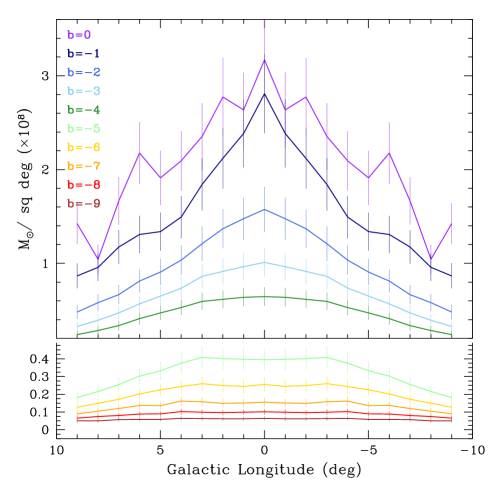
Figure 1: Stellar mass profile of the Galactic bulge, as a function of longitude, for different latitudes. The curves at low latitudes are shown on a different vertical scale, to increase visibility. This is a new version of Fig. 5 in Valenti et al. (2016) where we have imposed symmetry about the Galactic plane and about the bulge projected minor axis ($l=0$). Statistical uncertainties, coming from the Poisson fluctuation on the number of RC stars are $\sim$1%. Error bars of 15% of the data points are shown here, in order to account for the systematics, such as the IMF slope, the disk contamination and the adopted size of the RC box; see Valenti et al. (2016) for a discussion.

There are two important assumptions in this approach. The first is that the measurements of the total LF and the IMF for the bulge are correct as in Zoccali et al. (2003) and Zoccali et al. (2000), respectively. Because all the numbers needed for the calculation are given, new assumptions for the bulge LF and IMF allow one to derivate a new value for the bulge mass. For example, a new IMF was measured by Calamida et al. (2015), based on optical HST data, with proper motion decontamination from foreground disk stars. Their best fitting power law has a slope of $\alpha$=$-2.41$ for masses in the range 1$-$0.56 $M_{\odot}$ and $\alpha$=$-1.25$ in the range 0.56$-$0.15 $M_{\odot}$. By using this IMF instead of the Zoccali et al. (2000) one, and mantaining the assumptions for the brown dwarfs and the remnants, the total bulge stellar mass is $2.1\times 10^{10}$ $M_{\odot}$, consistent with the value derived in Valenti et al. (2016).

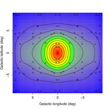
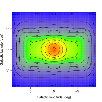
Figure 2: Number density maps of the MP (left) and MR (right) components, obtained by convolving the MP/MR relative fraction of stars from the metallicity distribution function, and the global stellar density map from Valenti et al. (2016). Open circles show the grid of fields used in the interpolation, resulting from folding the measurements in the GIBS fields with respect to both Galactic latitude and longitude. The maps are normalized to the same color scale. The figure is reproduced from Zoccali et al. (2017); see the original paper for details.

The second assumption is the fact that when we count stars in the RC+RGB region of the bulge CMD, we are indeed counting only bulge stars. The normalization between the stars counted in the whole VVV area and the bulge LF in the SOFI field in Zoccali et al. (2003) was done in a box of $\pm 1.5$ mag across the RC peak. These stars are used as tracers of the underlying bulge stellar density, which is a safe hypothesis unless there is another population, along the line of sight, that contributes to the counts in this range. In addition, the distance limits within which the stellar mass is measured are formally fixed by this $\pm 1.5$ mag interval across the RC. However, because this magnitude range corresponds to distance limits much larger than the bulge extension, they might include other components. In order to assess the impact of the adopted normalization box on the final estimation of the bulge total stellar mass, we repeated the calculation counting stars within $\pm 1.0$ mag, and within $\pm 0.5$ mag, across the RC peak. The resulting bulge mass is $1.93\times 10^{10}$ and $2.22\times 10^{10}$ $M_{\odot}$, respectively, consistent to the $2.0\pm 0.3\times 10^{10}$ $M_{\odot}$ given in Valenti et al. (2016), and well within the estimated uncertainty. In what follows we will use the latter value as total bulge stellar mass, when needed. However here we determine the relative contribution of the MP and MR component to the total stellar mass, which is independent from the value adopted for the latter.

In order to derive the density and mass profile for the bulge MP and MR components, separately, we combine Valenti’s results with the fractional density maps of MP and MR stars obtained by Zoccali et al. (2017) from the GIBS program. These maps were derived by imposing 4-fold spatial symmetry, about the Galactic plane, and about the projected minor axis. Given that i) the stellar density is mostly symmetric; and ii) we use symmetric maps from GIBS, we produce here a 4-fold averaged version of the mass profile from Valenti et al. (2016, their Fig.5), shown in Fig. 1. The figure shows a smooth increase of the bulge stellar mass when moving towards the Galactic center, with the presence of a boxy structure evident at latitudes $b$=$-4$,$-5$,$-6$. The zig-zag profile at $b$=0 is due to the observational complications of this region with much larger extinction (therefore more uncertain differential extinction correction), lower completeness and stronger foreground disk contamination.

3 The Projected density distribution of MP and MR stars

Figure 1 shows the projected profile of the total stellar mass contained in the bulge. As reviewed in the introduction, however, all the recent spectroscopic measurements, unambiguously show that the bulge contains two stellar components. They are best separated in the metallicity ([Fe/H]) distribution, but differ also in their spatial distribution, kinematical properties, and alpha-element abundances.

Zoccali et al. (2017) combined the relative fraction of the two populations, extracted from the GIBS metallicity distribution function in each of 26 bulge fields, with the stellar density map in Valenti et al. (2016). In this way they derived the stellar number density of each of the MP and MR component, in the 26 GIBS fields. By means of a 2D interpolation, they obtained a stellar density map for the MP and for the MR component, reproduced here in Fig. 2. The maps are 4-fold symmetric by construction (about the Galactic plane and about the $l=0$ axis), and they clearly show that the MP component is axysimmetric, i.e., circular when projected in the plane of the sky, while the MR one is markedly boxy. Because the maps are normalized to the same maximum density, they also show that the MP component reaches a slightly higher density in the central region. We emphasize that the innermost GIBS field is at ($l,b$)=($-0.26,-1.4$), where the fraction of MP stars with respect to the total is 53%. Therefore, the overabundance of MP stars in the center is marginal. It is however very interesting that MP stars are at least as abundant as MR ones in the Milky Way central region: this was a new and unexpected result of the GIBS project.

4 The mass fraction of MP and MR stars

The combination of the GIBS maps presented in the previous section and the stellar mass profile in Fig. 1 allows us to derive mass profiles for each of the MP and MR component, individually, that we list in the online Table 1. Conceptually, these carry the same information on the spatial distribution of MP and MR stars as the maps in Fig. 2. Converting these density maps in units of stellar mass, however, allows us to integrate them across the whole bulge area, hence deriving the percent contribution of the MP and MR component to the total stellar mass of the bulge.

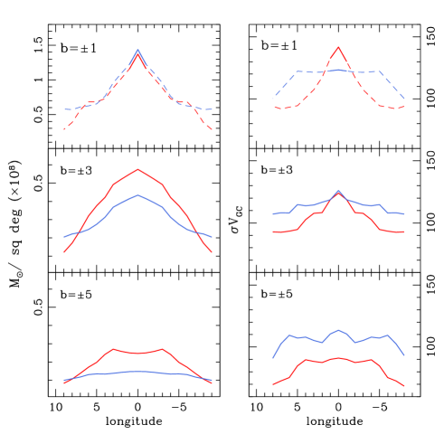
Figure 3: Left panels: stellar mass profile as a function of longitude, for three different latitudes, for MP (blue) and MR (red) stars, respectively. Right panels: same thing for the galactocentric radial velocity profile. At $b$=$\pm 1$ the curves are dashed, except at $l$=$0$, to remind the reader that they are constrained by a single field at ($l,b$)$\sim$($0,-1$), and -only through the interpolation- by the fields at $b$=$-2$).

The left panels of Fig. 3 show the mass profile with longitude, plotted at three representative latitudes, for the MP (blue) and MR (red) components, individually. These are the curves shown in navy blue ($b$=$-1$), azure ($b$=$-3$) and light green ($b$=$-5$) in Fig. 1 now splitted according to the MP/MR fraction in each point, as given by the GIBS maps.

As expected, MR stars are more abundant than MP stars in the bulge at latitudes $|b|$$>$$3$ (bottom and central panels). MR stars also show the boxy structure, at $b$=$\pm 5$. They are slighly underabundant at $b$=$-1$, where, we recall, we have data only for a single field at $l$$\sim$$0$, therefore we plot the profiles with dashed lines at other longitudes. MP stars, on the other hand, have a rather smooth trend, from a flat and marginal contribution at $|b|>5$ to a strong central concentration as we move closer to the Galactic plane. The mass profile of the two components at $b$=$0$ is not shown, because it would be just an interpolation, due to the lack of spectroscopic data at this latitude.

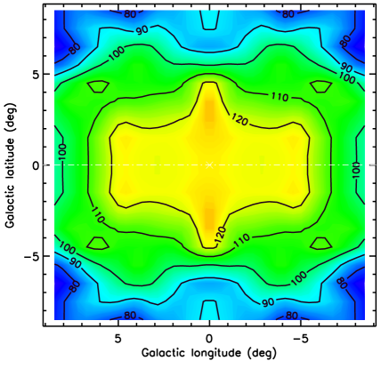
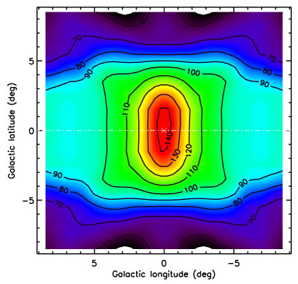
Figure 4: Spatial trends of the galactocentric radial velocity dispersion for the MP (left) and MR (right) component, respectively. The maps are the results of a linear interpolation between the measured value of the $\sigma$ for the two components, in the 26 GIBS fields. The maps are symmetric in longitude and latitude by construction, and they have been normalized to the same color scale. Contours show the value of $\sigma$, in km/s, in step of 10.

Integration of these profiles yields the stellar mass in each component, which turns out to be 52% in MR stars and 48% in MP stars. Although the presence of a MP component in the bulge has been established beyond any doubt by all the spectroscopic studies reviewed in the introduction, this is the first time that its contribution to the bulge stellar mass budget has been evaluated.

4.1 Comparison between mass and velocity dispersion

Something interesting to explore is the comparison between the stellar mass profile, directly inferred from the number of stars, and the radial velocity dispersion profile. The latter is widely used as tracer of the total (dynamical) mass, especially in extragalactic context, modulo some assuption on the spatial distribution of the stars (usually requiring fit of the surface brightness profile) and the distribution of the orbits.

A map of the global galactocentric radial velocity ($\sigma$), for the MP and MR components together, was published in Zoccali et al. (2014, their Fig. 11). Noticeably, the map shows a central $\sigma$-peak, reaching $\sim$140 km/s, that was not expected based on previous measurements in more external bulge regions (e.g., Howard et al., 2008; Freeman et al., 2013). The presence of the peak was rather firmly established by the GIBS data, as it resulted from measurement of the $\sigma$ in three independent fields, each sampling 441, 435 and 111 stars. However its spatial extension and symmetry about the Galactic plane was poorly constrained, since the 3 GIBS fields were rather close to each other, and all at negative latitudes. In a more recent paper, Valenti et al. 2018 (A&A, in press), used MUSE data to measure the $\sigma$ in four fields, two of which at $b$=$+2^{\circ}$, and confirmed both the presence and the symmetry of the peak.

Values for $\sigma$ of the MP and MR components, individually, have been measured by Zoccali et al. (2017), in each of the GIBS fields (c.f., their Fig. 11 and 12). By using the akima package in R (Akima 1978), we applied a bivariate linear interpolation to the irregular grid of 26 GIBS fields after imposing a 4-fold symmetry and derive spatial maps of sigma for MP and MR stars shown in Fig.4. We recall that this interpolation allow us to examine the run of a variable ($\sigma$ in this case) in strips at constant latitude, which would be impossible with the raw data because – in order to minimize extinction – the observed fields were not exactly on a regular grid. Second, the interpolation allows us to predict the value of $\sigma$ at any position intermediate between our fields. Third, it allows a straightforward comparison with IFU measurements of external, edge-on galaxies (Gonzalez et al., 2016).

The right panels of Fig. 3 show the trend of $\sigma$ for the MP (blue) and the MR (red) stars, as a function of longitude, at three constant latitudes (the same as for the mass trends on the left panels). Interestingly, the $\sigma$ has an opposite trend with respect to the mass (or to the stellar density). Namely, at intermediate heights from the Galactic plane, MR stars dominate the star counts, especially close to the projected minor axis ($l$=$0$). Their $\sigma$, however, is significantly lower than that of MP stars. This behaviour is reverted at $b$=$\pm 1$, where MP stars dominate the star counts, hence the stellar mass budget, but their $\sigma$ is lower than that of MR stars. In other words, at ($l,b$)=($0,-1$), MR stars have a significantly larger velocity dispersion, that does not correspond to a significantly larger contribution to the mass. This is because MR stars, arranged in a bar, have mostly elongated orbits, which increase the observed 1-D sigma. Curiously, this behaviour ir inverted at b=+/-5, where MP stars have a larger sigma although their contribution to the mass budget is lower.

Table 1: Percent contribution of MP and MR stars to the bulge stellar mass as a function of Galactic position.

$l$	$b$	% MP	% MR
$-9$	$-9$	0.0138	0.0100
$-9$	$-8$	0.0171	0.0143
$-9$	$-7$	0.0228	0.0200
$-9$	$-6$	0.0318	0.0280
….	….	….	….
Note: The full table is available online at CDS.

5 Conclusions

With the increasing amount of photometric and spectroscopic data over the last decade, the complexity of the Galactic bulge morphological, dynamical, and stellar population properties has become evident. In particular, one of the properties that has been largely discussed in the literature is the different behaviour of MP and MR bulge stars.

Although from a purely observational perspective, it is not possible to separate bulge populations on the basis of a given formation mechanism, in this study we used the fact that the metallicity distribution function can be separated in at least two populations in a statistically significant way. The separation between populations are consistently seen across the bulge and their variation can be quantified without any assumptions on their physical origin. Adequate numerical models and simulations are now available via which the characteristics of these two population can be linked to a partciular bulge formation process. However, one missing ingredient so far has been the relative contribution of the MP and MR populations to the total mass budget of the bulge.

In this study we derive this number for the first time by using two results presented recently by the GIBS and VVV surveys, namely the relative density distribution maps of MP and MR from (Zoccali et al., 2017) and the mass profile of the bulge from Valenti et al. (2016). We converted the GIBS stellar density maps of MP and MR populations into maps of stellar mass and integrate them across the entire bulge area to derive their relative contribution to the total stellar mass of the bulge. We find that the relative contribution to the total bulge mass comes in a 52% from MR stars and 48% from MP stars.

We also discuss the spatial variations of both the mass and radial velocity dispersion profiles of MP and MR components. We show that while MR stars dominate the star counts at intermediate latitudes ($b$$\sim$$-5$) their $\sigma$ is considerably lower than that of MP stars. This behaviour is reverted closer to the plane ($b$$\sim$$-1$) where MP stars are dominant but their $\sigma$ is lower than that of MR stars.

We note that the connection between the velocity dispersion and the mass is not direct, as it involves the orbit anisotropy and the spatial distribution of the stars. It is not the purpose of the present paper to infer the physical connection between the two. We here focus on presenting the data, emphasizing that they show complex trends that require detailed modeling to be understood. Proper motions are available from VVV in the $|b|$$<$3 region, and -very soon- from Gaia for the rest of the bulge, for the same stars for which we have radial velocities and metallicities, therefore in the near future bulge formation models can be constrained much better than before, hopefully allowing us to definitely discard some scenarios in favor of the others.