An exposition of the false confidence theorem
Iain Carmichael and Jonathan P Williams
University of North Carolina at Chapel Hill
Abstract
A recent paper presents the “false confidence theorem” (FCT) which has potentially broad implications for statistical inference using Bayesian posterior uncertainty. This theorem says that with arbitrarily large (sampling/frequentist) probability, there exists a set which does not contain the true parameter value, but which has arbitrarily large posterior probability. Since the use of Bayesian methods has become increasingly popular in applications of science, engineering, and business, it is critically important to understand when Bayesian procedures lead to problematic statistical inferences or interpretations. In this paper, we consider a number of examples demonstrating the paradoxical nature of false confidence to begin to understand the contexts in which the FCT does (and does not) play a meaningful role in statistical inference. Our examples illustrate that models involving marginalization to non-linear, not one-to-one functions of multiple parameters play a key role in more extreme manifestations of false confidence.
Keywords: Bayesian methods; belief functions; epistemic probability; Fieller’s theorem; foundations of statistics; Gleser-Hwang theorem; statistical inference
Corresponding Author: Jonathan Williams, jpwill@live.unc.edu
1 Introduction
In a recent paper, Balch, Martin & Ferson (2017) presents the phenomenon of “false confidence” associated with Bayesian posterior uncertainty. The authors come about the concept of false confidence from an alarming application to satellite collision risk analysis when estimating the posterior probability of the event that two satellites will collide. They found that increased measurement error of satellite trajectory data leads to decreased posterior probability of satellites colliding. Essentially, as more noise is introduced into trajectory measurements we become less certain about satellite trajectories, and thus the probability of two satellites colliding decreases. However, since a posterior probability is an additive belief function (probabilities of mutually exclusive and collectively exhaustive sets sum to one) the probability of the two satellites not colliding must increase accordingly, making their respective trajectories appear safer. When taken to the extreme, a large enough measurement error will cause an analyst to be (mistakenly) certain the satellites will not collide. Conversely, when viewed from a likelihood-based sampling distribution framework, more noise in the trajectory data suggests that the satellite trajectories are less certain and therefore are less likely to collide because of the infinitely large number of possible paths they could each take. This alternative interpretation is not problematic.
More on the specifics and importance of satellite collision risk analysis are provided in Balch et al. (2017). To study the mechanics behind what is happening at a more fundamental level the authors present what they term the “false confidence theorem” (FCT). This theorem says that with arbitrarily large (sampling/frequentist) probability, there exists a set which does not contain the true parameter value, but which has arbitrarily large posterior probability. Such a phenomenon is unsettling for a practitioner making inference based on a posterior distribution. Moreover, the authors prove that false confidence effects all types of epistemic uncertainty represented by additive probability measures. This includes Bayesian posterior probabilities, fiducial probabilities, and probabilities derived from most confidence distributions (Balch et al., 2017).
Our goal is to illustrate the intuition and mechanics of the FCT in simple examples so that we can begin to understand more complicated manifestations of the FCT. Such insight provides a particularly useful contribution to the literature as the use of Bayesian methods becomes more popular. Our contributions in this paper are the following.
First, we present a simple example to illustrate the mechanics of the FCT with the statistical problem of estimating the support parameter of the U distribution. This is an example in which the mathematics for the FCT can be worked out analytically and demonstrates where each piece in the statement of the FCT originates from. In most other situations the mathematics cannot be worked out analytically due to the fact that the typical posterior distribution function does not have a readily understood sampling distribution. In the Appendix we provide similar results for a one parameter Gaussian model.
Next, we show that the FCT manifests in an even more pronounced way by extending the first example to a two parameter model, i.e., U and U with , and considering the marginal posterior distribution of the parameter . This example alludes to the intuition that false confidence is likely at play in situations in which the Gleser-Hwang theorem applies (Gleser & Hwang, 1987). Such examples are characterized in the frequentist paradigm by exhibiting infinitely large confidence intervals required to obtain less than 100 percent coverage (Berger et al., 1999; Gleser & Hwang, 1987). One such famous problem appears in Fieller’s theorem (Fieller, 1954) which has been discussed as recently as the last two meetings of the Bayesian, Fiducial, and Frequentist Conference (2017, 2018), and in the forthcoming paper Fraser, Reid & Lin (2018).
Finally, we demonstrate that the manifestation of the FCT is immediately apparent in a problem related to Fieller’s theorem. We show that in reasonable situations the FCT applies to sets which would be concerning in practice. The contribution of such a striking example of false confidence is worrisome in an era in which Bernstein-von Mises type results are unhesitatingly appealed to even when it may not be appropriate (e.g., certain small sample situations). Such a phenomenon should be properly understood for the appropriate use of Bayesian methodology in practice.
Broadly, the axioms of probability laid down by Kolmogoroff (1933) have enabled a rich mathematical theory, however, their suitability for modeling epistemic uncertainty has been met with some discontent, particularly the axiom of additivity (Shafer, 2008). The issue with additivity is that it does not leave room for ignorance (i.e., events are either true or false) which is a major underpinning of the FCT. Theories of inference which weaken additivity assumptions include inferential models (Martin & Liu, 2016b) and imprecise probabilities (Weichselberger, 2000; Gong & Meng, 2017).
The paper is organized as follows. Section 2 presents and describes the FCT as given in Balch et al. (2017). Sections 3, 4, and 5 present and analyze the illustrative examples, and additional analysis is provided in the Appendix. The code to reproduce the numerical results presented in this paper is provided at https://github.com/idc9/FalseConfidence.
2 Main ideas
This section presents the false confidence theorem from Balch et al. (2017).
Theorem 1 (Balch, Martin & Ferson (2017)).
Consider a countably additive belief function characterized by an epistemic probability density function on (the parameter space), with respect to the Lebesgue measure, satisfying , for -almost all . Then, for any , any , and any , there exists a set with positive Lebesgue measure such that , and
| (1) |
While Theorem 1 pertains to any form of epistemic probability, for concreteness we will focus on Bayesian posterior probability. This amounts to considering situations in which
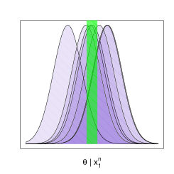
To better understand the statement of (1), Figure 1 demonstrates the pieces at play. The green region represents an example of a particular as described in the theorem, and each curve represents a particular realization of the posterior distribution (associated with ) over the sampling distribution of the data (associated with ).
Heuristically speaking, false confidence says that for some set, say , which does contain the true parameter value, the (epistemic) posterior probability can be made arbitrarily large with arbitrarily large (aleatory) sampling/frequentist probability, i.e., with respect to . Although the simple existence of such sets does not immediately raise concerns about statistical inference, for a given situation there may exist practically important sets, such as in the satellite collision risk analysis example of Balch et al. (2017). Note that these sets may be particularly concerning for finite sample sizes.
3 Uniform with Jeffreys’ prior
Here we investigate the FCT for uniformly distributed data where the goal is to estimate the support of the distribution. The motivation for considering this example is that it is simple enough that all of the mathematics can be worked out analytically. Let be a random sample from the U distribution where is an unknown parameter. Using the Jeffreys’ prior, , the posterior will be where is the maximum of the observed data (see Robert (2007)).
Suppose the true value of is and fix . Then by the proof of Theorem 1 (see Balch et al. (2017)) there exists such that
| (2) |
where , is the posterior law of (the additive belief function), and is the probability measure associated with the sampling distribution of the data. Note that in this example the Jefferys’ prior is a probability matching prior in the Welch-Peers sense (see Reid et al. (2003)); in particular, the interval is such that . Since the probability matching prior property in one-dimensions pertains to intervals, this fact provides further justification for considering the Jeffreys’ prior for analyzing sets of the form .
To compute the left side of (2), first re-express as
The second equality comes from the fact that the CDF of the distribution is given by . The third equality comes from considering the two cases of the indicator function, and the final equality comes from solving for .
Observe that (i.e., maximum order statistic of a U random sample) which gives . Accordingly,
| (3) |
Setting the right side of equation (3) equal to gives as a function of the , , and which satisfy the false confidence theorem. Specifically, we want to know if can be large enough to have a practically meaningful or harmful effect for statistical inference on . The relationship between and , for , is plotted in Figure 2.
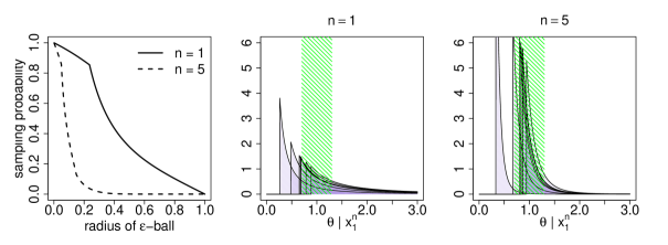
The leftmost panel in Figure 2 shows, for , the sampling probability (i.e., ) that the posterior probability of is less than , for -balls of various radii. For example, with the posterior probability of (which contains the true parameter value) will not exceed for , for more than 80 percent of realized data sets. This has the interpretation that the Bayesian test of “accept ” if and only if would be wrong more than 80 percent of the time.
Displayed on the next two panels of the figure are a few randomly observed realizations of the posterior density of , with a .3-ball around represented by the shaded green regions. The realizations of the posterior density are typically concentrated around the true value, . The next section demonstrates how to extend this example into a situation even more amenable to false confidence.
Remark 1.
This uniform example is one of the few simple examples where we can analytically work out the FCT in a straightforward manner. For example, for interval sets, equation (2) shows the posterior CDF needs an analytic sampling distribution.
4 Marginal posterior from two uniform distributions
Assume , and independently . Using the Jeffreys’ prior, gives and . Further, define the nonlinear functional , and derive the posterior distribution of as follows. By independence,
where the last expression results from the form of the Pareto CDF. If , then this equation simplifies to
and if , then the distribution function has the form
In both cases, the support of is .
For simplicity, attention will be restricted to the case. This analytic marginal posterior distribution function makes it simple to estimate , for and various values of , by simulating data sets and computing the empirical mean, i.e.,
| (4) |
where is the number of simulated data set pairs . This is done in Figure 3 for generated data sets. The true values are set at and which gives . Also displayed are a few realizations of the posterior density to illustrate where things go wrong.
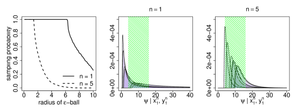
From Figure 3 it becomes clear how the FCT manifests. For , the -ball around with diameter even larger than 12 has posterior probability not exceeding , with sampling probability, , essentially equal to 1. As in the previous section, this has the interpretation that the Bayesian test of “accept ” if and only if would essentially always be wrong. Furthermore, in this case the Bayesian test would fail for an interval (containing the true parameter value) which has length longer than the magnitude of the true parameter value.
Although this is a toy example being used for pedagogical purposes, it is nonetheless alarming. One would hope that the small sample size of , while resulting in less posterior certainty about the location of the true parameter value, would be accompanied by more sampling variability/uncertainty. Rather Figure 3 implies the interpretation that we are certain about an answer which is in fact false. The center and rightmost panels of Figure 3 illuminate part of what is happening behind the scene; the posterior densities are typically diffuse around . The next section presents a more extreme instance of this phenomenon.
5 Marginal posterior from two Gaussian distributions
Assume , and independently . Suppose also that is known. Using independent Jeffreys’ priors, gives and . In this context, the nonlinear functional is related to the classical Fieller’s theorem in which infinite confidence intervals are required to attain frequentist coverage (Fieller, 1954; Gleser & Hwang, 1987; Berger et al., 1999).
The posterior density function for can be derived by transforming the two-dimensional posterior of into the space of and then computing the marginal distribution of . Observe that which gives the Jacobian for the transformation,
Then the joint posterior density has the form
Recalling the forms of the posterior densities for and , and integrating over gives
| (5) |
where the expectation is taken over .
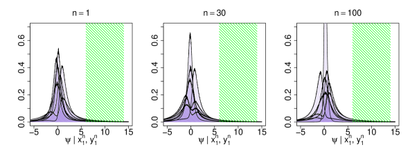
This marginal posterior is easily estimable, and , for and various values of , can be estimated with an approximating Riemann sum using equation (5). The estimated as a function of is displayed in Figures 4 and 5 for and , respectfully, and for various noise levels, . The true mean values are set at and which gives . Displayed in Figure 6 are a few random realizations of the posterior densities from (5), for various sample sizes, , with , to illustrate part of where things go wrong.

Remarkably, for almost all values of and considered in Figure 4 the Bayesian test of “accept ” if and only if would fail for as large as 8. Even considering the extreme choice of as in Figure 5, the sampling probability, , exceeds 80 percent chance (in the case of ) that for as large as 4, with .
A further illustration of what is happening is once again provided with random realizations of the marginal posterior densities presented in Figure 6. For this problem they heavily concentrate away from the true value . Consequentially, any inference on the true value of is sure to be misleading, and hence this situation is an extreme example of the manifestation of false confidence in a well-studied classical problem. Similar results hold for the manifestation of false confidence in other non-linear marginalization examples, e.g., the coefficient of variation which is discussed in the Appendix.

6 Concluding remarks and future work
There is currently little theoretical understanding of the phenomenon of false confidence or of when it plays a significant role in statistical analysis. We demonstrate ramifications of false confidence in standard, single parameter models as well as models involving the marginalization of multiple parameters. Our examples illustrate that models involving the marginalization to non-linear, not one-to-one functions of multiple parameters seem to play a key role in more extreme manifestations of false confidence. In future work we seek to gain an understanding of why the FCT is problematic in these situations.
7 Acknowledgments
The authors are grateful to Ryan Martin, Jan Hannig, and Samopriya Basu for many helpful comments, engaging conversations, and encouragement.
Appendix A Gaussian with Gaussian prior
Here we provide additional analysis to investigate the FCT for normally distributed data where the goal is to estimate the population mean. Let be a random sample from N, where is known, but is not and is the object of inference. Consider a prior distribution of .
Then the posterior distribution is where , , and . See Hoff (2009) for details.
Suppose the true value of is and fix . Proceeding through the analogous steps as in Sections 3-5 (i.e., we compute , and such that equation (2) holds),
where is the standard normal distribution function. Thus, equation (2) here is expressed as
| (6) |
Notice that the data appear in (6) only through , however, we cannot express as an analytic function of . If one could do so, then one could define the region of integration to evaluate the outside probability. Hence, a similar analytic expression to equation (3) cannot be immediately derived. Therefore, we use Monte Carlo simulation to better understand Equation (6).
To make matters concrete, fix , (i.e., ), and assign a diffuse prior . Using Monte-Carlo simulation we compute the value of satisfying equation (6) for a range of and between 0 and 1, and for the values of and .
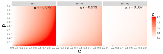
Figure 7 show a contour plot of as a function of and for three different values of . On each of these panels we mark the value of for and . This value of has the following meaning: with high sampling probability (), a large posterior probability () is assigned to the set which does not contain the true parameter, . In other words, over repeated sampling of the data, with high probably we will put a lot of belief on values that are at least away from the truth.
Appendix B Coefficient of variation
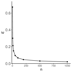
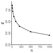
Here we consider the coefficient of variation model, and carry out a similar analysis as in the above section. Let where both and are unknown. Let be the parameter of interest. The true parameters are taken to be so . Figure 9 shows as a function of for and fixed ( and , respectively), and .
References
- (1)
- Balch et al. (2017) Balch, M. S., Martin, R. & Ferson, S. (2017), ‘Satellite conjunction analysis and the false confidence theorem’, arXiv preprint arXiv:1706.08565 .
- Berger et al. (1999) Berger, J. O., Liseo, B., Wolpert, R. L. et al. (1999), ‘Integrated likelihood methods for eliminating nuisance parameters’, Statistical Science 14(1), 1–28.
- Dempster (2008) Dempster, A. P. (2008), ‘The Dempster–Shafer calculus for statisticians’, International Journal of approximate reasoning 48(2), 365–377.
- Fieller (1954) Fieller, E. C. (1954), ‘Some problems in interval estimation’, Journal of the Royal Statistical Society. Series B (Methodological) pp. 175–185.
- Fraser et al. (2018) Fraser, D. A. S., Reid, N. & Lin, W. (2018), ‘When should modes of inference disagree? Some simple but challenging examples’, Annals of Applied Statistics: Special section in memory of Stephen E. Fienberg .
- Gleser & Hwang (1987) Gleser, L. J. & Hwang, J. T. (1987), ‘The nonexistence of 100 (1-)% confidence sets of finite expected diameter in errors-in-variables and related models’, The Annals of Statistics pp. 1351–1362.
- Gong & Meng (2017) Gong, R. & Meng, X.-L. (2017), ‘Judicious judgment meets unsettling updating: Dilation, sure loss, and Simpson’s paradox’, arXiv preprint arXiv:1712.08946 .
- Hoff (2009) Hoff, P. D. (2009), A first course in Bayesian statistical methods, Springer Science & Business Media.
- Klir (2005) Klir, G. J. (2005), Uncertainty and information: foundations of generalized information theory, John Wiley & Sons.
- Kolmogoroff (1933) Kolmogoroff, A. (1933), ‘Grundbegriffe der wahrscheinlichkeitsrechnung’.
- Martin & Liu (2016a) Martin, R. & Liu, C. (2016a), Inferential Models, Wiley Online Library.
- Martin & Liu (2016b) Martin, R. & Liu, C. (2016b), ‘Validity and the foundations of statistical inference’, arXiv preprint arXiv:1607.05051 .
- Reid et al. (2003) Reid, N., Mukerjee, R. & Fraser, D. (2003), ‘Some aspects of matching priors’, Lecture Notes-Monograph Series pp. 31–43.
- Robert (2007) Robert, C. (2007), The Bayesian choice: from decision-theoretic foundations to computational implementation, Springer Science & Business Media.
- Shafer (1976) Shafer, G. (1976), A mathematical theory of evidence, Vol. 42, Princeton university press.
- Shafer (2008) Shafer, G. (2008), Non-additive probabilities in the work of Bernoulli and Lambert, in ‘Classic Works of the Dempster-Shafer Theory of Belief Functions’, Springer, pp. 117–182.
- Weichselberger (2000) Weichselberger, K. (2000), ‘The theory of interval-probability as a unifying concept for uncertainty’, International Journal of Approximate Reasoning 24(2-3), 149–170.