Massively Parallel Simulations of Binary Black Hole Intermediate-Mass-Ratio Inspirals

Abstract

We present a highly-scalable framework that targets problems of interest to the numerical relativity and broader astrophysics communities. This framework combines a parallel octree-refined adaptive mesh with a wavelet adaptive multiresolution and a physics module to solve the Einstein equations of general relativity in the BSSNOK formulation. The goal of this work is to perform advanced, massively parallel numerical simulations of Intermediate Mass Ratio Inspirals (IMRIs) of binary black holes with mass ratios on the order of 100:1. These studies will be used to generate waveforms as used in LIGO data analysis and to calibrate semi-analytical approximate methods. Our framework consists of a distributed memory octree-based adaptive meshing framework in conjunction with a node-local code generator. The code generator makes our code portable across different architectures. The equations corresponding to the target application are written in symbolic notation and generators for different architectures can be added independent of the application. Additionally, this symbolic interface also makes our code extensible, and as such has been designed to easily accommodate many existing algorithms in astrophysics for plasma dynamics and radiation hydrodynamics. Our adaptive meshing algorithms and data-structures have been optimized for modern architectures with deep memory hierarchies. This enables our framework to have achieve excellent performance and scalability on modern leadership architectures. We demonstrate excellent weak scalability up to $131K$ cores on ORNL’s Titan for binary mergers for mass ratios up to $100$.

83-08,85-08

1 Introduction

Figure 1: This figure illustrates the calculation of a single Runge-Kutta time step, computing the solution at the advanced time, $u_{n+1}$, from data at the previous time step, $u_{n}$. For computational efficiency, spatial and time derivatives are evaluated on equispaced blocks (unzipped); a sparse grid constructed from wavelet coefficients is used for communication and to store the final solution (zipped). For each RK stage $s$ we perform the unzip operation which results in a sequence of blocks which are used to compute the solution on the internal block ($\blacksquare$), using the padding values at the block boundary ($\blacksquare$) followed by a zip operation in between RK stages while the final update (i.e. next time step) performed using the zip version of the variables. Note that the re-meshing is performed as needed based on the wavelet expansion of the current solution (see §3.5).

In 2015, shortly after beginning its first observing run, the Laser Interferometer Gravitational-Wave Observatory (LIGO) [1, 82] made the first direct detection of gravitational waves from the merger of two black holes [7]. Since that time, gravitational waves from four other binary black hole mergers [8, 6, 11, 12] have been detected by LIGO and the European Virgo detectors [2, 14]. In August 2017, LIGO and Virgo detected gravitational waves from the merger of a neutron star binary [4]. This latter detection was particularly exciting because electromagnetic radiation from the resulting gamma-ray burst was detected by the Fermi Gamma-Ray Burst Monitor [44] and INTEGRAL [78], as well as by several other observatories [10]. The combination of gravitational and electromagnetic observations of binary mergers will give new insight into the physics of black holes (BHs) and neutron stars [13, 17, 9]. As the sensitivity of the LIGO detectors improves, gravitational wave detections will increase in frequency and open a new era of gravitational wave astronomy.

Gravitational waves carry the imprint of their origins within the complicated pattern of their waveform. The information therein can be untangled through a careful comparison of the gravitational wave signal with a library of possible waveforms constructed using approximate methods and results from numerical simulations. Indeed, waveform information from numerical relativity is particularly important for certain binary black hole configurations. Examples include binary black holes with arbitrary spin configurations [20], binaries with orbital eccentricity, and binaries for which the black holes have very different masses [47, 54].

In this paper, we use $q$ to denote the mass ratio of a binary as $q\equiv m_{1}/m_{2}$, where $m_{1}\geq m_{2}$. At this time, very few large mass-ratio BH binaries ($q\gg 1$) have been studied in numerical relativity, compared to studies with nearly equal mass ($q\approx 1$) [59, 84]. Codes developed for $q\approx 1$ binaries are accurate and well tuned, so the problem is well-understood and numerical results are confidently used in the LIGO data-analysis pipeline. However, configurations with large $q$ remain largely beyond the capabilities of current techniques in numerical relativity. Examples include Intermediate Mass-Ratio Inspiral (IMRI) binaries and are characterized roughly by $q\simeq 100$. It is estimated that about 5% of the detections in LIGO might come from IMRIs [3, 43].

For an IMRI, the size of the smaller black hole adds an extra length-scale to the problem, compared to the $q\approx 1$ case. The need to resolve this scale, together with the large range other important length scales for the binary system, makes this a very challenging computational problem. It requires a highly adaptive and efficient computational algorithm tuned to handle binaries with large mass ratios. While BH evolutions with $q=100$ have been performed [62, 61, 85] previously, they were not completed till the merger event or simulated direct head-on collisions. Therefore the above simulations are not satisfactory to be useful toward gravitational wave analysis.

The central goal of our effort is to create a general purpose framework to study the evolution of spacetimes with black holes or neutron stars, including binary black holes with large mass ratios up to $q\simeq 100$. Here we present our portable, highly-scalable, extensible, and easy-to-use framework for general relativity (GR) simulations that will be forward-compatible with next-generation heterogeneous clusters.

We build on our octree-based adaptive mesh refinement (AMR) framework Dendro  [87, 75] to support Wavelet Adaptive Multiresolution (WAMR) [69, 68, 35]. The fast wavelet transform can be used to create a sparse representation of functions that retains sharp features and an a priori error bound.

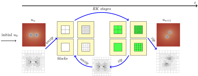
The high-level overview of our approach is illustrated in Figure 1. We use an efficient block-decomposition of the distributed octree to produce a collection of overlapping regular grids (at different levels of refinement, see §3.3.6 ).

The Einstein equations of general relativity describe the spacetime geometry and, expressed in terms of the BSSNOK formulation [81, 66], where each spatial grid point is associated with $24$ unknowns. Given their complexity and a desire for portable code, we auto-generate the core computational kernels automatically from the equations written in symbolic Python (SymPy  [53], see §3.4). The auto-generated code is applied at the block-level and is therefore very efficient and enables portability. The equations are integrated in time using the method of lines with a Runge-Kutta (RK) integrator.

The key contributions of this work include:

Wavelet Adaptive GR. To the best of our knowledge, comparable codes use simple models of adaptivity, i.e., structured adaptivity, block adaptivity, or logically uniform grids [38, 67, 26, 99]. We present a novel computational GR framework (Dendro-GR) which uses octree-based Adaptive Multiresolution (AMR) grids, where the adaptivity is guided by wavelet expansion [97, 95, 69, 68, 49] of the functions represented in the underlying grid. We refer this as Wavelet Adaptive Multiresolution (WAMR). This is the first highly adaptive fully relativistic—i.e., including the full Einstein equations—code with an arbitrary localized adaptive mesh. For example for a mass ratio of $q=1$, we use approximately 7x fewer degrees of freedom for the same accuracy compared to the block adaptivity (via Carpet [31]).

Automatic code generation. Given the complexity of the Einstein equations, we have developed an automatic code generation framework for GR using SymPy that automatically generates architecture-optimized codes. This greatly improves code portability, use by domain scientists and the ability to add additional constraints and checks to validate the code.

Performance. We developed a new parallel search algorithm TreeSearch (see §3.3.5), to improve the efficiency of octree meshing. We also developed efficient unzip and zip operations (block-decomposition of WAMR grid to produce collection of overlapping regular grids, see §3.3.6) to allow the application of the core computational kernels to small process-local regular blocks. This improves performance as well as performance portability in conjunction with our automatic code generation. Local calculations on regular blocks allows us to use established, existing numerical methods for the Einstein equations, and in future work, the relativistic fluid equations and radiation hydrodynamics equations.

Simulations. We demonstrate the ability to scale to large mass ratios, enabling simulations and extraction of gravitational waves for mass ratios as high as $100$.

Implementation Dendro-GR is implemented in C++ using MPI except for the automatic code generation framework which is implemented using SymPy. Our code is freely available at https://github.com/paralab/Dendro-GR under the MIT license.

Organization of the paper: The rest of the paper is organized as follows. In §2, we give a brief motivation on the importance of numerical simulations of BH binary configurations and a quick overview of the existing state-of-the-art approaches in the field of numerical relativity. In §3, we present the methodology used in Dendro-GR  in detail and how it is efficient compared to the existing approaches. In §4, we discuss the experimental setup, strong and weak scalability of our approach, including a detailed comparison study with the state-of-the-art Einstein Toolkit [38] package. In §5, we conclude with directions for future work.

2 Background

In this section, we discuss the motivating applications and summarize the most relevant work of other groups in this area. As gravitational waves pass through the Earth, their effect on matter is extremely small. LIGO searches for gravitational waves by using laser interferometry to detect changes in the relative position of mirrors, to a precision of four orders of magnitude smaller than an atomic nucleus. The gravitational wavesignals in the detector are often smaller in magnitude than noise from other sources, but the signals can be extracted using matched filtering [77], which uses a library of hundreds of candidate waveforms that are convolved with the data. Including complete numerical waveforms in the waveform library is important to maximize the detection rate of IMRIs in LIGO-class detectors [83].

Figure 2: (left) A example of the adaptive mesh created by Dendro for the binary black-hole system. (right) the hierarchical wavelet grids generated for the binary black hole system.

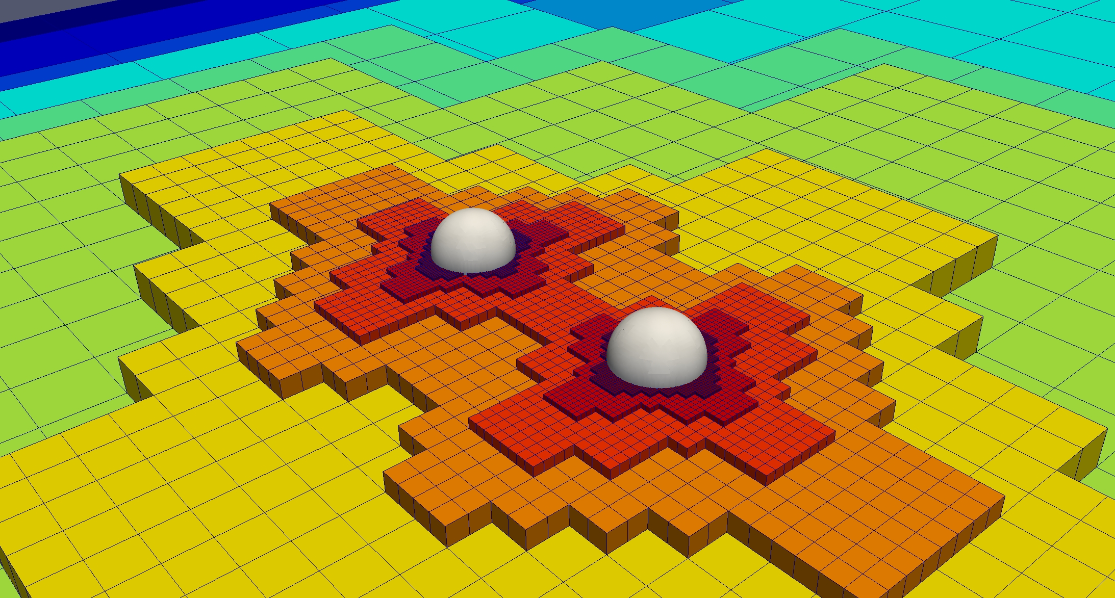
The Einstein equations of general relativity describe how the geometry of spacetime curves in response to the presence and motion of matter and energy. The Einstein equations contain both hyperbolic evolution equations and elliptic constraint equations. Commonly the hyperbolic equations are solved, and the elliptic equations are used to ”monitor” the quality of the solution [18, 79] (see Appendix A). The solution at time $t$ for evolution equations should satisfy Hamiltonian and momentum constraints (i.e. compute the $l_{2}$ norm of the constraint violation) in order to verify the solution is physically valid. While the equations can be formulated in many different ways, few formulations are well-suited for numerical work. One such formulation is the BSSNOK formulation [21]. The BSSNOK evolution equations are a set of strongly hyperbolic [76] coupled PDEs that are first-order in time and second-order in space. A brief summary of the BSSNOK  with constraint equations is provided in the Appendix A.

Several computer codes have been developed to solve the Einstein equations for binary BH and neutron star systems. One of the oldest open source projects in this community is the Cactus Computational Toolkit [29, 45], that provides a modular infrastructure for solving time-dependent PDEs in parallel using structured grids. Modules for specific tasks, known as thorns in Cactus parlance, can be shared and combined to produce a sophisticated evolution code. The Einstein Toolkit (ET) is a suite of community-developed thorns for relativistic physics [38].

It includes thorns for constructing binary BH initial data, for evolving the Einstein equations and/or the relativistic fluid equations, and for data analysis. Similar codes include [91, 57, 56, 67, 39]. Further, the SXS collaboration has developed SpEC [89], a spectral code for solving the Einstein equations that has produced the longest and most-accurate binary waveforms to date.

The challenge of running on modern massively parallel computers is pushing new developments in numerical relativity. The use of structured grids with block-based AMR, such as used by Cactus/ET and similar codes, is not ideal for new massively parallel architectures and can lead to inefficient refinement (refined in the regions where coarser representation is sufficient), especially for $q\gg 1$. One new approach for the ET  is the SENR project [74, 64], that uses coordinate systems adapted to the binary BHs to eliminate the need for AMR. Another approach is to use discontinuous Galerkin (DG) methods, that requires less communication between processes. The first three-dimensional ADER-DG simulations of the Einstein equations were performed by Dumbser et al. [37].

The SXS collaboration is developing the SpECTRE code [55, 73] that uses task-based parallelism and DG. Thus far only results for the relativistic MHD equations have been published.

We have chosen to focus on one type of BH binary that is particularly difficult to study both numerically and with semi-analytical approximations. These are IMRIs, BH binaries with mass ratios with $50\lesssim q\lesssim 1000$. The successful numerical simulation of IMRIs and their predicted gravitational wave signal is difficult because of the large difference in the two mass-scales in the problem. Gravitational waves must be resolvable far from the binary system while the region around both black holes must also be accurately simulated. Standard approaches [38, 67, 26, 99] to black hole simulations often include mesh adaptivity by which necessary resolution is concentrated in dynamic regions.

The Dendro-GR code uses octree grids based on the wavelet expansion [97, 95, 69, 68, 49], that produces refinement regions adapted to features in the solution with a minimum number of points. This is important for problems with fine-scale features that are not spatially localized (i.e. adaptivity of the grid is not pre-determined based on the spatial locations of BHs), or problems with widely disparate scales, such as IMRIs. Moreover, the numerical methods used in this paper are based on the conventional finite difference methods that have been widely used and tested (see, §3.1). This allows existing numerical approaches to be more easily adapted to the Dendro-GR  through symbolic code generation framework. Given the scale of our problem, even with adaptivity, massively parallel computing resources are required. We build our Dendro-GR  framework based on our parallel adaptive meshing framework Dendro [88, 87] and extend it to support numerical relativity codes with finite differencing.

A key reason to develop scalable codes is that as the relative differences in masses becomes larger ($\sim 100\times$), the computational requirements will grow significantly, potentially requiring exascale resources. A simple calculation illustrates how spatial resolution requirements increase with $q$. A convenient measure for the size of a black hole is the radius of its event horizon, which is proportional to its mass. In a black hole binary, the mass of the smallest black hole effectively sets the minimum length scale for the simulation. The total mass of the binary $M=m_{1}+m_{2}$ is a global scaling parameter and is typically fixed to a constant value. Then the mass of the smaller black hole can be written $m_{2}=M/(q+1)$, showing that the minimum resolution scale for the binary is inversely proportional to the mass ratio. In three spatial dimensions the number of points required to resolve the smallest black hole grows as $q^{3}$. This presents both a challenging problem in computational relativity as well as a challenge for high-performance computing. The successful scaling of our code is a first step in this direction.

3 Methodology

Research in relativistic astrophysics requires specialized computational models for gravitational, plasma, and nuclear physics. The massively parallel infrastructure that we propose is compatible with the standard finite difference or finite volume discretizations that are currently used in these communities. We solve the BSSNOK equations using conventional finite-difference discretizations, standard gauges, and puncture initial data (see §3.1). We also adapt them to specific computer hardware and cache sizes using our new symbolic interface (see §3.4). While this paper focuses on the vacuum Einstein equations, we are currently working to add modules for the relativistic MHD equations, nuclear equations of state, and neutrino leakage.

3.1 Numerical Methods

There is extensive literature on solving the BSSNOK equations in general relativity, and some general reviews include [18, 79, 72]. In this section we briefly outline our particular choices for solving BSSNOK  equations. We write the BSSNOK equations in terms of the conformal factor $\chi$ [30]. We use the parameterization of the “$1+\log$” slicing condition and the $\Gamma$-driver shift used in [67]. Spatial derivatives are calculated using finite difference operators that are ${\rm O}(h^{4})$ in the grid spacing, $h$, with upwind derivatives for Lie derivative terms [100]. We calculate derivatives for the Ricci tensor and enforce the algebraic constraints as described in [26]. Outgoing radiative boundary conditions are applied to each BSSNOK function. The BSSNOK equations are integrated in time using an explicit RK scheme. The solution at each point is integrated with a single global times step, that is set by the smallest grid spacing and the Courant condition [33]. While we support $3$rd and $4$ order RK, the tests in this paper were done using $3$rd order RK with Courant factor $\lambda=0.1$. Kreiss-Oliger dissipation is added [58, 18] to the solution to eliminate high-frequency noise that might be generated near the black hole singularities.

3.2 Wavelet Adaptive Multiresolution

WAMR uses a basis of interpolating wavelets to create a sparse, quasi-structured grid that naturally adapts to the features of the solution [69, 68, 35]. This grid adaptivity is realized by expanding functions using the fast wavelet transform [49], and thresholding (i.e. based on a user-specified tolerance $\epsilon>0$) the solution to create a sparse representation that retains small-scale features [36]. In WAMR, we start with the coarsest representation ($V_{0}$) of a given function $f$. Then we compute wavelet coefficients based on the interpolation error as a result of the interpolation of $f$ from the coarser representation to the next finer representation ($V_{1}$). Hence the wavelet coefficient denotes the interpolation error that occurs when $f$ is constructed from the immediate coarser level. The sparse representation of the function $f$ is computed based on the user-specified tolerance and removing the spatial points whose wavelet coefficients are within the specified threshold (see Figure 3).

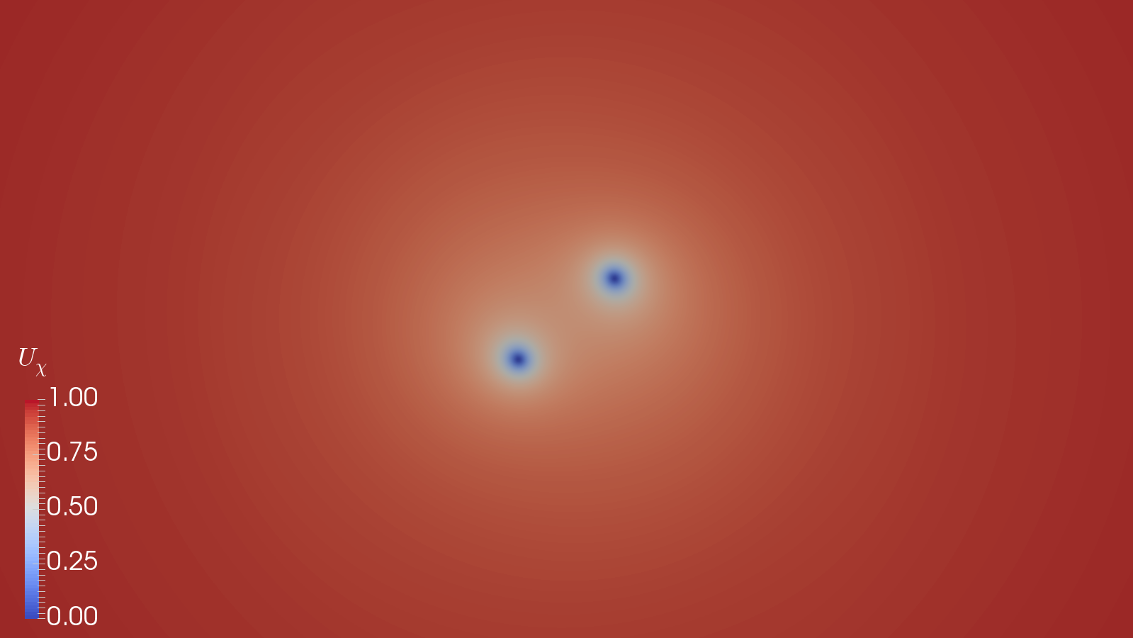
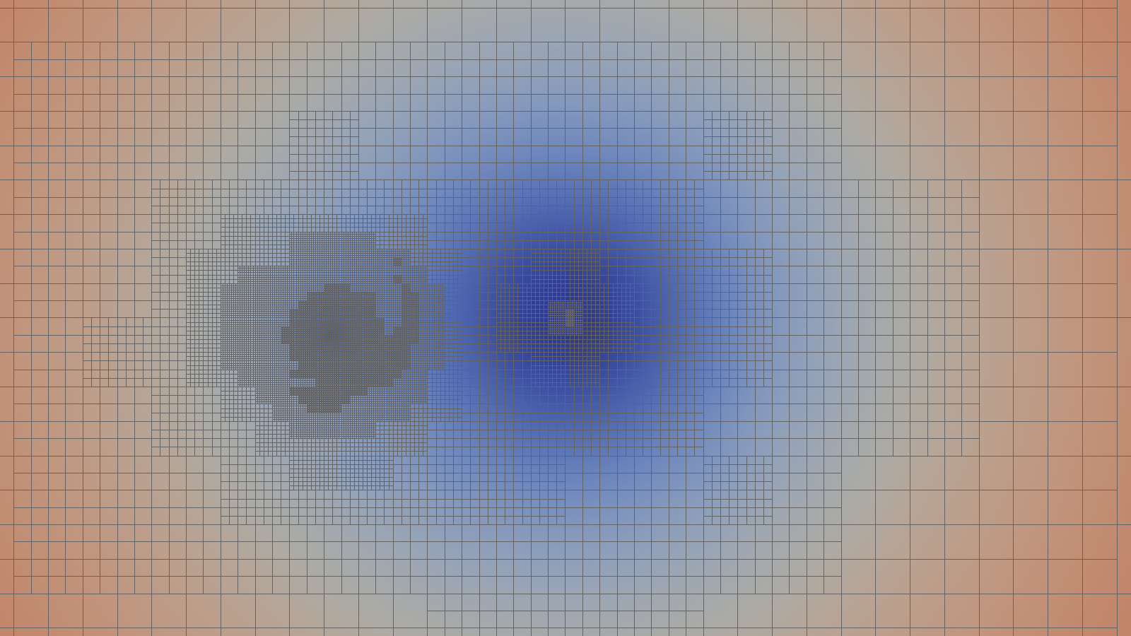
Wavelet basis functions are localized (i.e. have compact support) both spatially and with respect to scale. In comparison, spectral bases are infinitely differentiable, but have global support; basis functions used in finite difference or finite element methods have small compact support, but poor continuity properties. As an example, in Figure 2 we show a binary black hole spacetime generated with WAMR using Dendro-GR.

Figure 3: For a given function $f:V\rightarrow\mathcal{R}$ let $V_{i}\subset V$ be the finite dimensional approximation of $f$ (see Figure 3). As number of nodes increases (i.e. going from $V_{i}$ to $V_{i+1}$) for each additional node introduced, we compute wavelet coefficients based on the absolute difference between $f(V_{i,k})$ and interpolated value from previous level $f(V_{i-1,:})$ (see Figure 3). In Figure 3 shows the chosen nodes that violate specified wavelet tolerance $epsilon$ and these nodal wavelets are stored as the sparse/wavelet representation of function $f$ (see Figure 3).

Wavelets encode solution features at different scales very efficiently, a characteristic that leads to many applications in data and image compression [16]. Studies of WAMR have shown the method to be significantly more efficient in terms of computational cost when compared with traditional numerical schemes [70]. The wavelet amplitudes also provide a direct measure of the local approximation error and serve as a refinement criterion. We work simultaneously with both the point and wavelet representations [24, 94, 71, 97, 95, 96]. This gives wavelet methods some of the same advantages as DG [90, 27], including exponential convergence. Combining the sparse grid generated by the truncated wavelet expansion with Dendro yields a wavelet adaptive multiresolution method that enables a promising improvement for simulating the mergers of compact object binaries.

3.3 Computational Framework

We now give an overview of the approach that Dendro-GR takes in order to obtain excellent scalability in the context of the WAMR method. Our parallel WAMR framework is based on adaptive spatial octrees [86, 41] where the adaptivity is determined by the hierarchical computation of wavelet coefficients and a user-specified tolerance. The construction of adaptive octrees is similar to other octree-codes such that every element at level $l$ gets replaced by eight finer (smaller) elements (i.e. level $l+1$) if the computed wavelet coefficient is larger than the user-specified tolerance. The main steps in building the parallel octree-WAMR framework are partitioning, construction and enforcement of constraints on the relative sizes of neighboring octants, and meshing. By meshing, we refer to the process of building required data structures to perform numerical computations on a topological octree (see §3.3.5).

3.3.1 Preliminaries

Octree based spatial subdivisions are fairly common in computational science applications [28, 75, 15, 98, 22], due to their simplicity and scalability. Here we present some basic concepts and notation related to octrees used in this paper. A distributed octree $\mathcal{T}$ consists of $p$ subtrees $\tau_{i},i=1,\ldots,p$, where $p$ is the number of processes and $\mathcal{T}=\cup\tau_{i}$. For an octant $e$, $F(e)$ denotes the faces, $E(e)$ denotes the edges and $V(e)$ denotes the vertices of $e$. The neighbors of $e$ are given by $N(e)=N_{F}(e)\cup N_{E}(e)\cup N_{V}(e)$, where $N_{F}(e)$ denotes the octants that share only a face, $N_{E}(e)$ denotes the octants that share only an edge and $N_{V}(e)$ denotes the octants that share only a vertex with $e$. If $\tau_{i}$ spans the sub-domain $\omega_{i}\subset\Omega$, the boundary octant set, $bdy(\tau_{i})$, consists of those octants that share faces, edges and vertices with $\partial\omega_{i}$. Correspondingly, the set of interior octants is given by $int(\tau_{i})=\tau_{i}\setminus bdy(\tau_{i})$. Finally, the octree $\tau$ is said to be $2:1$ balanced if and only if for any $e_{k}\in\tau$ where $level(e_{k})=l_{k}$, $\forall e\in N(e_{k})$ then $level(e)=max(l_{k}\pm 1,0)$. In this work, we enforce a $2:1$ balance constraint on our octrees.

3.3.2 Octree partitioning

The problem size or the local number of octants varies significantly during WAMR based octree construction (in WAMR we start with the coarsest representation and add grid points until all the wavelet coefficients are within the specified tolerance ), balancing, meshing and during the simulation as well.

This necessitates efficient partitioning of the octree to make it load balanced. We use a space-filling curve (SFC) [93] based partitioning scheme [41], specifically the Hilbert-curve. An SFC specifies a surjective mapping from the one-dimensional space to higher dimensional space. This can be used to enforce an SFC based ordering operator on higher dimensional space. The Hilbert ordering maps higher dimensional data (octants) to a 1D curve which makes the process of partitioning trivial. The key challenge is to order the octants or regions according to the SFC, usually performed using an ordering function and sorting algorithm. This approach is easily parallelized using efficient parallel sorting algorithms such as SampleSort [42] and BitonicSort [51] which is the approach used by several state-of-the-art packages [28, 87, 88]. We use a comparison-free SFC sorting algorithm TreeSort, based on the radix sort. In TreeSort, we start with the root octant and hierarchically split each dimension while bucketing points for each octant and reordering the buckets, based on the specified SFC ordering (see Figure 4). This is performed recursively on depth-first traversal until we reach all the leaf nodes (see Algorithm 1). Additional details on our partitioning algorithm can be found in [41].

Figure 4: Bucketing each point and reordering the buckets based on the SFC ordering at each level $l$ with top-down traversal. Each color-coded point is represented by its $x$ and $y$ coordinates. From the MSD-Radix perspective, we start with the most-significant bit for both the $x$ and $y$ coordinates and progressively bucket (order) the points based on these. The bits are colored based on the points and turn black as they get used to (partially) order the points.

Algorithm 1 TreeSort

1:A list of points or regions $W$, the starting level $l_{1}$ and the ending level $l_{2}$

2:$W$ is reordered according to the SFC.

3:$counts[]\leftarrow 0$ $\triangleright$ $|counts|=2^{d}$, 8 for $3D$

4:for $w\in W$ do

5:    increment $counts[child\_num(w)]$

6:$counts[]\leftarrow R_{h}(counts)$ $\triangleright$ Permute counts using SFC ordering

7:offsets [] $\leftarrow scan(counts)$

8:for $w\in W$ do

9:    $i\leftarrow child\_num(w)$

10:    append $w$ to $W_{i}$ at offsets$[i]$

11:    increment offset$[i]$

12:if $l_{1}>l_{2}$ then

13:    for $i:=1:2^{d}$ do

14:        TreeSort($W_{i},l_{1}-1,l_{2}$) $\triangleright$ local sort     

15:return $W$

3.3.3 Octree Construction and Refinement

The octree construction is based on expanding user-specified functions (e.g. initial conditions for a hyperbolic differential equation ) via the wavelet transformation and truncating the expansion (i.e. stopping the refinement at that level) when the coefficients are smaller than a user-specified tolerance $\epsilon>0$. Intuitively, the wavelet coefficient measures the failure of the field to be interpolated from the coarser level. In distributed memory, all processes start from the root and refine until at least $p^{2}$ octants are produced, where $p$ denotes the number of processors. These are equally partitioned across all processes. Subsequent refinements happen in an element-local fashion, and are embarrassingly parallel. A re-partition is performed at the end of construction to load-balance.

3.3.4 $2:1$ Balancing

Following the octree construction, we enforce a $2:1$ balance condition. This makes subsequent operations (§3.3.5, §3.3.6 and §3.3.7 ) simpler without affecting the adaptive properties. Our balancing algorithm is an updated version of the algorithm presented in [87]. The octree is divided into small blocks, that are independently balanced by preemptively generating all balancing octants [23], followed by ripple propagation for balancing across the blocks. The ripple propagation inter-block balancing approach performs poorly at large levels of parallelism, and we instead extend the generation algorithm [23]. The basic idea is to generate all balancing octants for a given octant and then to remove duplicates. While this approach can generate up to 8x the number of total octants, it is very simple and highly parallel. We ensure that the overall algorithm works efficiently, by relying on our TreeSort algorithm to sort and remove duplicates periodically, ensuring that the number of octants generated remains small.

3.3.5 Meshing

By meshing or mesh generation we simply refer to the construction of data structures required to perform numerical computations on topological octree data. As mentioned in §3.1, we use $4^{th}$ order Finite Differences (FD) with 5-point stencils for $\partial_{i},\partial_{ij}^{2}$, and 7-point stencils for $\partial_{i},i,j\in[1,2,3]$ with upwind/downwind and Kriess-Oliger derivatives. We use a $RK$ time integrator with the method of lines to solve the BSSNOK  equations. In this section, we present the data structure choices that we have made and how everything comes together to perform numerical computations on adaptive octree data to evolve the BSSNOK  equations in time.

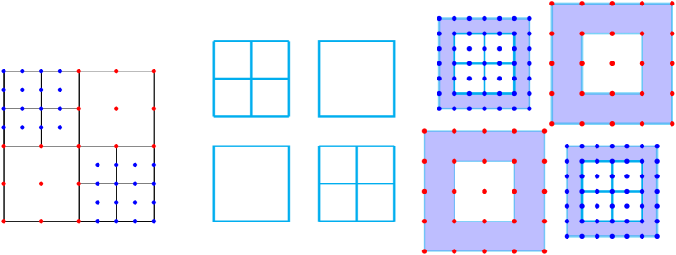
Embedding nodal information on an octree: In order to perform FD computations on an octree, we need to embed spatial/nodal points for each octant. Assuming that we want to perform $d^{th}$ order FD computations, we uniformly place $(d+1)\times(d+1)\times(d+1)$ points for each octant. In our simulations, we have used $d=4$ since we are performing $4^{th}$ order FD computations, but the meshing algorithms presented in the paper are valid for any integer value of $d$. The nodes obtained by uniform node placement are referred to as octant local nodes  ($V_{D}$). Octants that share a face or an edge will have duplicate nodal points in $V_{D}$, and we need to remove the duplicate nodes from $V_{D}$ to get shared octant nodes  ($V_{S}$) for several reasons. 1).$V_{S}$ has a lower memory footprint compared to $V_{D}$. 2). A function representation, on a $V_{D}$, can be discontinuous due to node duplications, unless function values of duplicate nodes are synchronized. Due to the above reasons, we use $V_{S}$ as our prime nodal representation (also referred as zipped representation) of the octree. Since the octrees are generated with WAMR, finding the duplicate and hanging nodes (see Figure 7) from $V_{D}$ becomes non-trivial and requires an octant level neighborhood data structure which is referred to as octant to octant (o2o) mapping. Also, we need an additional mapping to map the octants to the $V_{S}$ representation which is referred to as octant to nodal (o2n) mapping.

Figure 5: A $2D$ example of octant local nodes  (in the center) and shared octant nodes (the rightmost figure) nodal representation (with $d=2$, where $d$ denotes the order of FD computations) of the adaptive quadtree shown in the leftmost figure. Note that in octant local nodes  representation nodes are local to each octant and contain duplicate nodes. By removing all the duplicate and hanging nodes by the rule of nodal ownership we get the shared octant nodes  representation. Note that the nodes are color coded based on the octant level.

We now describe the methods for building these maps. Note that for the mesh generation, we assume the input is a complete, ordered and 2:1 balanced octree.

Figure 6: For a given ordered octree $\tau$ and a set of keys (leftmost figure), TreeSearch  performs the traversal in a top-down order over the set of keys, while flagging $k_{2},k_{4},k_{5}$ at the level $1$ split, $k_{3}$ at level $2$ split, and $k_{1}$ at level $3$ split.

TreeSearch: amortized search operations on octrees: The common approach for building the maps o2o and o2n  is to generate keys corresponding to the location of neighboring octants and to perform a parallel binary search on the octree and build the maps [87, 28]. Assuming the number of keys we need to search is $\mathcal{O}(n)$, where $n$ is the number of octants, the cost of performing binary searches for all the keys is $\mathcal{O}(n\log(n))$. The $\log(n)$ term corresponding to the binary search is inefficient due to poor memory access and can end up being very expensive for large $n$. We present an alternative TreeSearch, with better memory access for performing search operations on an ordered octree. To the best of our knowledge this algorithm is new. The approach used in TreeSearch  is influenced by radix sort, where we traverse the set of search keys and the octree in the space filling curve (SFC) induced ordering. As shown in Figure 6, we start at level $1$, split and calculate bucket counts $|b|$ generated by the split while reordering the keys in the same traversal order dictated by the SFC. $|b|=1$ suggests that octant $e\in\tau$. At this point, $b$ is an ancestor of all keys $k\in b$, and we have found the index the octant. In contrast with the other approaches, TreeSearch  performs a serial traversal over the set of keys and the elements of the ordered octree leading to better memory and cache performance (see Algorithm 2). Although the complexity for this approach is still $\mathcal{O}(n\log(n))$, it can be thought as performing $\log n$ streaming sweeps over the $\mathcal{O}(n)$ octants, leading to better performance.

Algorithm 2 TreeSearch: Searching in octrees

1:ordered octree $\tau$ on domain $\Gamma$, list keys $\mathcal{K}\in\Gamma$,

2:list keys $\mathcal{K}\in\Gamma$ with flagged search results.

3:$oct\_counts[]\leftarrow 0$

4:$key\_counts[]\leftarrow 0$ $\triangleright$ $|oct\_counts|=|key\_counts|=2^{d}$, 8 for $3D$

5:for $e\in\tau$ do

6:    increment $oct\_counts[child\_num(e)]$

7:for $k\in\mathcal{K}$ do

8:    increment $key\_counts[child\_num(k)]$

9:    $k.result\leftarrow\emptyset$

10:$oct\_counts[],$key_counts []$\leftarrow R_{h}(oct\_counts,key\_counts)$ $\triangleright$ Permute counts using SFC ordering

11:offsets_oct [] $\leftarrow scan(oct\_counts)$

12:offsets_key [] $\leftarrow scan(key\_counts)$

13:for $k\in\mathcal{K}$ do

14:    $i\leftarrow child\_num(k)$

15:    append $k$ to $\mathcal{K}_{i}$ at offsets_key$[i]$

16:    increment offset_key$[i]$

17:for $i:=1:2^{d}$ do

18:    if $oct\_counts>1$ then

19:        TreeSearch($\mathcal{K}_{i},\tau_{i}$)

20:    else

21:        for $k\in\mathcal{K}_{i}$ do

22:           $k.result\leftarrow$ offset_oct$[i]$             

23:return $\mathcal{K}$

Ghost/Halo octants: Since the octree is partitioned into disjoint subtrees owned by different processes, we need access to a layer of octants belonging to other processes. These are commonly known as the halo or a ghost layer. The computation of ghost octants can be reduced to a distributed search problem where each octant in each partition generates a set of keys that can be searched for to determine the ghost layer. Note that after the ghost-exchange all search operations are local to each partition/process.

Octant to octant map (o2o): Once the ghost layer has been received, we compute the o2o map by performing local searches using TreeSearch  for the neighbors (along $x,y$ and $z$ axes directions) of all octants and storing their indices. Therefore for an given octant $e\in\tau$, $\textsc{o2o}(e)=\{e_{1},...,e_{8}\}$ will return $8$ neighbor octants of $e$. The algorithm for the o2o map construction is listed in Algorithm 3.

Algorithm 3 BuildOctantToOctant: compute o2o

1:an ordered 2:1 balanced distributed octree $\mathcal{T}$ on $\Gamma$, $\mathit{comm}$, $p$, $p_{r}$ of current task in $\mathit{comm}$.

2:compute o2o

3:$\hat{\tau_{p_{r}}}\leftarrow\textsc{ComputeGhostOctants}(\mathcal{T},comm,p,p_{r})$

4:o2o$~{}\leftarrow\emptyset$

5:$keys[]\leftarrow$ compute $\mathcal{K}(\hat{\tau_{pr}})$

6:$\textsc{TreeSearch}(\hat{\tau_{p_{r}}},keys)$

7:for $key\in keys$ do

8:    if $key$ is found then

9:        o2o[key.owner][key.neighbor]=key.result     

10:return o2o

Figure 7: An example of a hanging face and a hanging edge where in both cases octant ($\blacksquare$) has a hanging face (left figure) and a hanging edge (right figure) with octant ($\blacksquare$). Nodes on the hanging face/edge are mapped to the larger octant and the hanging nodal values are obtained via interpolation. Note that for illustrative purposes, the two octants are drawn separately, but are contiguous.

Algorithm 4 BuildOctantToNodal: Octant to nodal map generation - o2n

1:an ordered 2:1 balanced distributed octree $\mathcal{T}$ on $\Gamma$, $\mathit{comm}$, $p$, $p_{r}$ of current task in $\mathit{comm}$.

2:compute o2n

3:$\hat{\tau_{p_{r}}}\leftarrow\textsc{ComputeGhostOctants}(\mathcal{T},comm,p,p_{r})$

4:o2n$~{}[]\leftarrow$ $initialize(\mathcal{V}_{L})$ $\triangleright$ o2n initialized with octant local nodes

5:$\mathcal{V}_{S}\leftarrow$ $\mathcal{V}_{L}\setminus\mathcal{V}_{D}$

6:for $e\in\hat{\tau_{k}}$ do

7:    for $v\in N_{d}(e)$ do $\triangleright$ $N_{d}(e)$ denotes $(d+1)^{3}$ nodes of $e$

8:        $owner\_idx\leftarrow$ compute $\mathcal{O}(v)$

9:        o2n$~{}\leftarrow owner\_idx$     

10:return o2n

Octant to nodal map (o2n): Since we use the shared octant nodes  ($V_{S}$)  to store all the simulation variables, we need a mapping between the underlying octree and $V_{S}$. The o2n  map simply specifies the subset $v$ of shared octant nodes  nodes (where $|v|=(d+1)^{3}$) of a given octant $e\in\tau$. When computing o2n  we initially start with octant to the $V_{D}$ map which is trivially constructed by definition of $V_{D}$. In order to remove duplicate nodes (see Figure 5), we need to define a globally consistent rule of nodal ownership. The ownership of nodes which lie on a hanging face or edge (see Figure 7) will belong to the coarser octant (since they can be interpolated from coarser level) while ties and non-hanging nodal ownership are determined by the SFC ordering of octants. Duplicate nodes are removed from the octant local nodes ($V_{D}$) to obtain the shared octant nodes ($V_{S}$) while modifying octant to $V_{D}$ map to generate octant to $V_{S}$ map (o2n). The overview of computing o2n  map is presented in Algorithm 4. By the assumption that the octree is 2:1 balanced, the owner nodes (see Figure 7) of hanging nodes cannot be hanging, which simplifies the construction of the o2n  mapping.

Figure 8: A simplistic example of octree to block decomposition and unzip  operation. The leftmost figure shows the considering adaptive octree with shared octant nodes  and its block decomposition is shown in the middle. Note that the given octree is decomposed into four regular blocks of different sizes. The rightmost figure shows the decomposed blocks padded with values coming from neighboring octants with interpolation if needed. In order to perform unzip  operation both o2o and o2n mappings are used.

$\displaystyle\partial_{t}\alpha$ $\displaystyle=$ $\displaystyle\mathcal{L}_{\beta}\alpha-2\alpha K,$ $\displaystyle\partial_{t}\beta^{i}$ $\displaystyle=$ $\displaystyle\lambda_{2}\beta^{j}\,\partial_{j}\beta^{i}+\frac{3}{4}f(\alpha)B^{i}$ $\displaystyle\partial_{t}B^{i}$ $\displaystyle=$ $\displaystyle\partial_{t}\tilde{\Gamma}^{i}-\eta B^{i}+\lambda_{3}\beta^{j}\,\partial_{j}B^{i}-\lambda_{4}\beta^{j}\,\partial_{j}\tilde{\Gamma}^{i}$ $\displaystyle\partial_{t}\tilde{\gamma}_{ij}$ $\displaystyle=$ $\displaystyle\mathcal{L}_{\beta}\tilde{\gamma}_{ij}-2\alpha\tilde{A}_{ij},$ $\displaystyle\partial_{t}\chi$ $\displaystyle=$ $\displaystyle\mathcal{L}_{\beta}\chi+\frac{2}{3}\chi\left(\alpha K-\partial_{a}\beta^{a}\right)$ $\displaystyle\partial_{t}\tilde{A}_{ij}$ $\displaystyle=$ $\displaystyle\mathcal{L}_{\beta}\tilde{A}_{ij}+\chi\left(-D_{i}D_{j}\alpha+\alpha R_{ij}\right)^{TF}+$ $\displaystyle\alpha\left(K\tilde{A}_{ij}-2\tilde{A}_{ik}\tilde{A}^{k}_{\,j}\right),$ $\displaystyle\partial_{t}K$ $\displaystyle=$ $\displaystyle\beta^{k}\partial_{k}K-D^{i}D_{i}\alpha+$ $\displaystyle\alpha\left(\tilde{A}_{ij}\tilde{A}^{ij}+\frac{1}{3}K^{2}\right),$ $\displaystyle\partial_{t}\tilde{\Gamma}^{i}$ $\displaystyle=$ $\displaystyle\tilde{\gamma}^{jk}\partial_{j}\partial_{k}\beta^{i}+\frac{1}{3}\tilde{\gamma}^{ij}\partial_{j}\partial_{k}\beta^{k}+\beta^{j}\partial_{j}\tilde{\Gamma}^{i}-$ $\displaystyle\tilde{\Gamma}^{j}\partial_{j}\beta^{i}+\frac{2}{3}\tilde{\Gamma}^{i}\partial_{j}\beta^{j}-2\tilde{A}^{ij}\partial_{j}\alpha+$ $\displaystyle 2\alpha\left(\tilde{\Gamma^{i}}_{jk}\tilde{A}^{jk}-\frac{3}{2\chi}\tilde{A}^{ij}\partial_{j}\chi-\frac{2}{3}\tilde{\gamma}^{ij}\partial_{j}K\right)$         from DENDRO_sym import *    a_rhs = Dendro.Lie(b, a) - 2*a*K    b_rhs = [3/4 * f(a) * B[i] +    l2*vec_j_del_j(b, b[i])    for i in e_i]    l2*vec_j_del_j(b, b[i])   for i in e_i]       B_rhs = [Gt_rhs[i] - eta * B[i] +   l3 * vec_j_del_j(b, B[i]) -   l4 * vec_j_del_j(b, Gt[i])   for i in e_i]       gt_rhs =  Dendro.Lie(b, gt) - 2*a*At       chi_rhs = Dendro.Lie(b, chi) +   2/3*chi*(a*K - del_j(b))       At_rhs = Dendro.Lie(b, At) + chi *   Dendro.TF(-DiDj(a) +   a*Dendro.Ricci) +   a*(K*At -2*At_ikAtKj)       K_rhs = vec_k_del_k(K) - DIDi(a) +   a*(1/3*K*K + A_ij_A_IJ(At))       

Figure 9: The left panel shows the BSSNOK formulation of the Einstein equations. These are tensor equations, with indices $i,j,\ldots$ taking the values $1,2,3$. On the right we show the Dendro_sym code for these equations. Dendro_sym uses SymPy and other tools to generate optimized C++ code to evaluate the equations. Note that $\mathcal{L}_{\beta},\ D,\ \partial$ denote Lie derivative, covariant derivative and partial derivative respectively, and we have excluded $\partial_{t}\Gamma^{i}$ from Dendro_sym to save space. (See [21, 18] for more information about the equations and the differential operators.)

3.3.6 unzip  and zip  Operations:

All simulation variables are stored in their most compact or zipped representation, i.e., without any duplication. Due to the use of 2:1 balanced adaptive octrees, performing FD computation on the octree is non-trivial. In order to overcome the above, we use unzip representation (a representation in between shared octant nodes  and octant local nodes). Any given adaptive octree $\tau_{k}$ can be decomposed into a set of regular grid blocks of different sizes–basically a set of octants that are all at the same level of refinement. Due to the memory allocation and performance, we enforce block sizes to be powers of two. In order to perform stencil operations on these blocks, we need information from neighboring blocks, similar to the ghost layer which is required by the distributed case. In the context of blocks, we refer to this layer as the padding. During meshing, we compute and save the octree-to-block decomposition, i.e., which octants are grouped together as a block. The computation of octree-to-block decomposition primarily involves a top-down traversal over the local octants and stopping when all elements in the block are at the same level. In order to convert the zipped to the unzipped representation, we copy the data from the zipped representation to the blocks with padding region. This involves copying the data within the block, and copying–potentially with interpolation–from neighboring octants. Nodes on the block boundary which are hanging need to be interpolated during the copy. The 2:1 balance condition guarantees that at most a single interpolation is performed for any given octant.

The stencil and other update operations are only performed on the block internal while the padding region is read-only. At the end of the update, the simulation variables are zipped back, i.e., injected back to the zipped representation. This step does not involve any interpolations or communication and is very fast. Note that several key operations such as RK update and inter-process communications operate using the zip representation, and are extremely efficient which is depicted in strong and weak scaling results (see Figures 13 and 14). There are several additional advantages for unzipped representation. 1). unzipped representation decouples the octree adaptivity from the FD computations. 2). The block representation enables code portability and enables to perform architecture specific optimizations.

Although, several similar approaches [19, 31] exist for zip and unzip operations, these approaches rely on structured or block structured adaptivity. In contrast to existing approaches we have designed efficient scalable data structures to perform zip and unzip operations on fully adaptive $2:1$ balanced grids.

3.3.7 re-mesh  and inter-grid transfer operations

As the BHs orbit around each other, we need to remesh so that maximum refinement occurs around the singularities. We do not enforce maximum refinement at singularities artificially, this is automatically performed by WAMR due to the fact that, BSSNOK  variables might not even be $C^{0}$ continuous at BH locations. The unzip  representation at the end of the time-step is used to determine the wavelet coefficients for each block based on a user-specified threshold. This allows us to tag each octant with refine, coarsen or no change. This is used to remesh, followed by a repartition to ensure load-balance. Once the re-mesh operation is performed we transfer the solution from old mesh to the newly generate mesh using interpolations as needed. We refer to this is inter-grid transfer and this is done via interpolations or injections at the block level.

3.4 Symbolic interface and code generation

The Einstein equations are a set of non-linear, coupled, partial differential equations. Upon discretization, one can end up with 24 or more equations with thousands of terms. Sustainability, code optimizations and keeping it relevant for architectural changes are additional difficulties. To address these issues, we have developed a symbolic interface for Dendro-GR. Note that there are several significant attempts such as Kranc[50] and NRPy [74] on symbolic code generation for computational relativity due to the complexity of the BSSNOK  equations. We leverage symbolic Python (SymPy) as the backend for this along with the Python package cog to embed Python code within our application-level C++ code. The Dendro_sym package allows us to write the discretized versions of the equations similar to how they are written mathematically and enable improved usability for Dendro-GR  users. An example for the BSSNOK equations are shown in Figure 9, with the equations on the left and the corresponding Python code on the right.

There are several advantages to using a symbolic interface like Dendro_sym for the application-specific equations. First, it improves the portability of the code by separating the high-level description of the equations from the low-level optimizations, which can be handled by architecture-specific code generators. We support avx2 code generators and are working on developing a CUDA generator as well. Since these are applied at a block level, it is straightforward to schedule these blocks across cores or GPUs. Note that the auto-generated code consists of several derivative terms that are spatially dependent as well as other point-wise update operations. We perform common subexpression elimination (CSE) [32, 63] to minimize the number of operations. Additionally, we auto-vectorize the pointwise operations and have specialized implementations based on the stencil-structure for the derivative terms.

Algorithm 5 Overview of our approach

1:$M\leftarrow$ initialize mesh $\triangleright$ §3.3.5

2:$u\leftarrow$ initialize variables $(M)$

3:while $t<T$ do

4:    for $r=1:3$ do $\triangleright$ RK stages

5:        $B,\hat{u}\leftarrow\text{Unzip}(M,u)$ $\triangleright$ §3.3.6

6:        for $b\in B$ do

7:           Compute derivatives $\triangleright$ Machine generated code §3.4

8:           Compute $\hat{u}_{rhs}(b)$ $\triangleright$ Machine generated code §3.4         

9:        $u_{rhs}\leftarrow\text{Zip}(M,B,\hat{u}_{rhs})$ $\triangleright$ §3.3.6

10:        RK update     

11:    $t\leftarrow t+dt$

12:    if need remesh $M$ then $\triangleright$ §3.3.7

13:        $M^{\prime}\leftarrow$ remesh($M$)

14:        $u^{\prime}\leftarrow$ Intergid_Transfer$(M,M^{\prime},u)$ $\triangleright$ §3.3.7     

3.5 Putting everything together

We use an RK time stepper to perform the time evolution. The algorithmic choices we have made in Dendro-GR  support arbitrary $d^{th}$ order RK time integration. The initial octree is constructed based on the WAMR method until the generated grid convergers to capture specified initial data, which is followed by the $2:1$ octree balancing and mesh generation phase which result in all the distributed data structures that are needed to perform ghost/halo exchange, unzip  and zip  operations. A given RK stage is computed by performing unzip  operations with overlapped exchange of the ghost layer for the evolution variables, computation of the derivatives and right-hand-side (rhs) using the code generated by the symbolic framework for all local blocks and finally performing zip  operation to get the computed zipped rhs variables. The RK update is then performed on the zipped variables. After a specified number of timesteps, we compute the wavelet coefficient for the current solution represented on the grid, and perform remesh and inter-grid transfer operations if the underlying octree grid needs to be changed. Note that wavelet computation for the grid is a local to each process while remesh and inter-grid transfer need interprocess communication. An complete outline of our approach for simulating binary BH mergers demonstrating how the various components come together is listed in Algorithm 5 and illustrated in Figure 1.

In the Appendix A.1 we present an example on how to use Dendro-GR  framework to solve simpler (compared to BSSNOK) NLSM  equations. NLSM  example also serves as an additional test to ensure all the Dendro-GR  modules are working and integrated correctly. We also performed additional tests with NLSM  with zero source term result in the standard linear wave equation which enables to perform convergence testing with the analytical solution.

4 Results

In this section we perform a thorough evaluation of our code, including detailed comparisons with the Einstein Toolkit. We first describe the machines used for these experiments followed by results demonstrating the improvements to Dendro and comparisons with Einstein Toolkit. Finally, we push our code to the limit of extreme adaptability to demonstrate its capability, using cases that are currently–to the best of our knowledge–beyond the capability of Einstein Toolkit.

Figure 10: Comparison between Einstein Toolkit  and Dendro-GR without factoring in adaptivity (i.e. both Einstein Toolkit  and Dendro-GR  support uniform grids.). For a fixed tolerance, we expand the domain for a $1:1$ mass-ratio simulation such that both Einstein Toolkit  and Dendro-GR have roughly the same number of dofs. We present both weak and strong scaling results using both codes. On the left table are results from Dendro-GR and from Einstein Toolkit  on the right. In the middle, we plot a representative strong and weak scaling curve for each code. The Dendro-GR  scaling is plotted in green (lighter shade for weak) and blue for Einstein Toolkit. The corresponding data entries are also marked in the tables. Note that the rows represent strong scaling and the diagonal entries represent weak scaling results and runtime is reported in seconds$(s)$.

Experimental Setup: The large scalability experiments reported in this paper were performed on Titan and Stampede2. Titan is a Cray XK7 supercomputer at Oak Ridge National Laboratory (ORNL) with a total of 18,688 nodes, each consisting of a single 16-core AMD Opteron 6200 series processor, with a total of 299,008 cores. Each node has 32GB of memory. It has a Gemini interconnect and 600TB of memory across all nodes. Stampede2  is the flagship supercomputer at the Texas Advanced Computing Center (TACC), University of Texas at Austin. It has $1,736$ Intel Xeon Platinum 8160 (SKX) compute nodes with $2\times 24$ cores and 192GB of RAM per node. Stampede2 has a 100Gb/sec Intel Omni-Path (OPA) interconnect in a fat tree topology. We used the SKX nodes for the experiments reported in this work.

Implementation Details: The Dendro-GR framework is written in C++ using MPI. The symbolic interface and code generation module uses symbolic Python (SymPy). In the comparisons with the Einstein Toolkit, we have used Cactus v4.2.3 and the Tesla release of the Einstein Toolkit. We integrated the BSSNOK equations with third-order RK for all comparisons in this paper. The constraint analysis, apparent horizon finder, and output were turned off for these runs.

unbalanced octants	balanced octants	2:1 balance ([87]) (s)	2:1 balance (Dendro-GR ) (s)
3K	5K	0.0087	0.0043
33K	59K	0.0908	0.0541
338K	553K	0.7951	0.5461
3M	5M	7.7938	6.9313
6M	11M	16.1828	14.7374

Table 1: Comparison study for 2:1 balancing approach used in [87] and the new balancing approach in a single core in Stampede2 (SKX node), with varying input octree sizes ranging from $3K$ to $6M$ octants.

Figure 11: Comparison of std::bsearch with partial ordering operator $<$ and comparison free TreeSearch  approach for performing, varying number of keys on $33M$ sorted complete octree using single core in Stampede2  SKX node.

Figure 12: Comparison between ET  and Dendro-GR for number of spatial points with increasing mass ratios. Note that these are not from complete simulations and the size of the problem as well as the time per RK-step is likely to increase, but it illustrates the rate of increase for both approaches. Parameters for the above experiment generated such that total mass of black holes equals to $1$ and the separation distance is $32$ for all cases and maxdepth  is set in a way that the spatial discretization $dx<\frac{\min(m_{1},m_{2})}{16}$ where $m1,m2$ denotes the individual masses of black holes.

4.1 Meshing Performance

In this section, we briefly present results for the improved scalability and performance of the proposed balancing and meshing algorithms. In Table 1, we list the improvement in enforcing 2:1 balancing by using TreeSort instead of the ripple propagation used in [87]. We present only single core results, as the algorithmic changes are for the sequential portions of the algorithms. In Table 1 we demonstrate significant savings for a range of problems sizes.

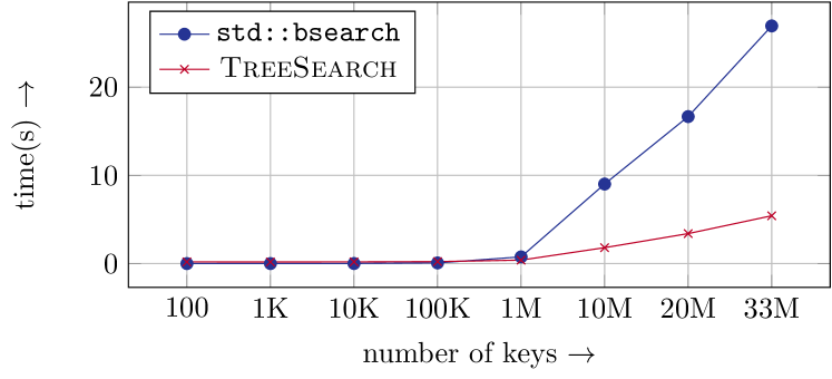
Similarly, significant savings are also obtained by the use of TreeSearch compared to the use of binary searches for the various search operations needed for meshing. In this experiment, we searched for $k$ keys in an array of size $n=33M$ octants. This size was chosen based on the average grain size we used in our experiments. Note that for meshing, $k=\mathcal{O}(n)$, and therefore we plot results up to $k=n$. Having a large array that is being searched in (large $n$), results in the first few steps of the binary search resulting in cache misses affecting overall performance. TreeSearch utilizes the deep memory hierarchy in a more effective fashion, but because of the additional work involved in sorting, requires a minimum number of keys to be searched for before it is cheaper. This can be seen in our results plotted in Figure 11, where TreeSearch scales better than std::bsearch, and is faster for $k>1M$. Given the number of keys being searched for during meshing, TreeSearch improves the overall meshing performance and scalability significantly.

4.2 Correctness of Code

We performed a number of tests to assess the correctness of our code, including simulations of static (Appendix B.9) and boosted black holes (Appendix B.10), as well as comparisons to other codes. To verify the automatic generation of the computer code for the BSSNOK equations, we evaluated these equations using arbitrary analytic functions of order unity over a grid of points, and compared the results to a known solution. The L2-norms of the error are equivalent to machine zero, given the limitations of finite-precision arithmetic. Additional results on the correctness are presented in Appendix B.6.

Figure 13: Weak scaling results in ORNL’s Titan for $RK/(dof/p)$ (averaged over 10 steps) where $RK,dof,p$ denotes the time for single $RK$ step, degrees of freedom, and number of cores respectively, with derivative computation (deriv), right hand side (rhs) computation, unzip cost, wavelet computation (wavelets) and communication cost (comm) with the average of 1.41M unknowns per core where the number of cores ranging from $32$ to $131,072$ cores on $8,192$ nodes where the largest problem having $206$ Billion unknowns. Above results are generated with mass ratio $\mu=10$ with maxdepth  18 and wavelet tolerance of $10^{-6}$. Note that the unknowns per core have a slight variation since with WAMR we do not have explicit control over the grid size and WAMR decides the refinement region on the mesh based on the how wavelets behave during the time evolution. This is why we have reported normalized $RK$ with $dof/p$ metrics to report accurate weak scaling results.

Figure 14: Strong scaling results in ORNL’s Titan for a single RK step (averaged over 10 steps) with derivative computation (deriv), right hand side (rhs) computation, unzip cost and communication cost (comm) for a fixed problem size of $10.5B$ unknowns where the number of cores ranging from $4,096$ to $65,536$ cores on $4096$ nodes. Note that for strong scaling results re-meshing is disabled in order to keep the problem size fixed.

4.3 Comparison with Einstein Toolkit

We compare our code with the BSSNOK formulation implemented in ET. The AMR driver for Cactus, Carpet [40], only supports block adaptivity. Therefore, we would expect Dendro-GR  to require fewer degrees of freedom (dof) for a given simulation and consequently be faster. Although ET  uses vectorization for improved performance [45], Dendro-GR  outperforms ET. Note that for all comparison studies with Einstein Toolkit , we have used the non-vectorized version of the Dendro-GR generated code. To highlight the improvements over ET, we perform two independent experiments. First, we compare the performance of both codes without adaptivity, and then in a separate experiment we show that Dendro-GR  provides a more efficient adaptivity and scaling than Carpet.

Uniform Grid Tests: In Figure 10, we present a comparison between Dendro-GR  and ET. This uses a regular grid for ET, and serves to highlight the efficiency of the Dendro-GR code including the overhead of adaptivity (i.e., zip and unzip). These runs were performed on Stampede2, and we show strong and weak scaling for both codes. Although both codes demonstrate good scaling, the performance (as measured by the time for one complete timestep) is better for Dendro-GR at higher core counts. Einstein Toolkit has better performance for large number of unknowns per core at low core counts. This effectively captures the overhead of zip and unzip compared to an efficient and mature code. For cases with higher core counts as well as smaller number of unknowns per core, Dendro-GR performs better. This is largely due to better cache utilization due to blocking, that largely compensates for the overhead of zip/unzip. Additionally, Dendro-GR  demonstrates better strong and weak scaling. The plot in Figure 10 highlights the strong and weak scaling of both codes for a representative grain and problem size. Dendro-GR  scales well far beyond the $3072$ cores, as shown in Figure 13 and discussed in §4.4.

Octree Adaptivity vs. Block Adaptivity: As motivated earlier, we wish to perform simulations of binary black hole mergers with large mass-ratios, $q\simeq 100$. Large mass-ratios require extensive refinement, increasing the number of spatial degrees of freedom.For an example let’s assume an equal mass binary requires a certain resolution for the BSSN equations, about 100 points per BH in each dimension. For a BH 100 times smaller, we need a resolution equivalent to 1/10,000 times the total mass and $100\times$ more time steps. The consequent high computational cost is the primary reason that current catalogs of numerical waveforms contain templates with a maximum mass ratio of $q<10$ [25, 48, 52].

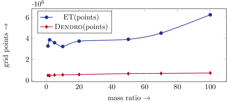
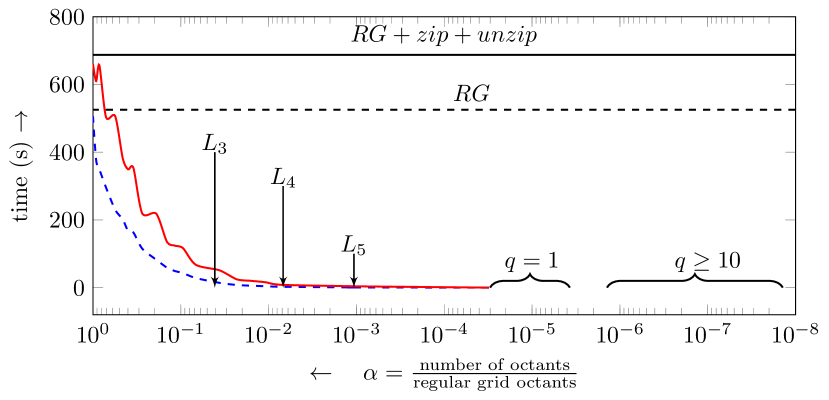
The efficient adaptivity of Dendro  is a big advantage over the block adaptivity of the ET. To assess the effect of adaptivity on code performance, we compared both codes for increasing mass-ratios from $q=1$–$100$, measuring the dofs, as shown in Figure 12. As the mass ratio increases, the number of dofs for ET increases much more rapidly than for Dendro-GR. While these results capture the differences at the beginning of the simulation, they are representative of the full simulation in terms of comparing the two codes. Because of better adaptivity and better scalability, Dendro-GR  keeps the cost of a single RK-step fairly flat as we scale up from $q=1$–$100$ mass-ratio. In Table 2 we present the number of cores needed to maintain a $24K$ unknowns per core with increasing mass ratio using Dendro-GR  framework. Finally, to illustrate the advantages of octree-adaptivity over block-adaptivity, even with the overhead of zip/unzip, we plot the reduction in runtime for 10 timesteps for different levels of adaptivity in Figure 15. Based on these results, it is clear that zip/unzip  with adaptivity can benefit especially for simulation of large mass ratio configurations and that the overhead is about $20\%$ even for a full regular grid simulation. These results further support our findings in Figure 10.

Figure 15: An illustrative single core example to evaluate the overhead of zip/unzip operations to evaluate BSSN equations on a sequence of octree grids over 10 timesteps. The parameter $\alpha$ denotes the ratio between the number of octants to the number of regular grid octants for MaxDepth $8$. Hence moving towards the right direction on $x$ axis the octree grids converge towards a regular grid. $RG$ and $RG+zip+unzip$ denotes the baseline performance for regular grid computations and regular grid computation with zip/unzip overhead respectively. The shaded $q=1$ region denotes the $\alpha$ value for an equal mass ratio simulation until the merger event using MaxDepth $12$ over $2\times 10^{5}$ timesteps. For larger mass ratio runs the MaxDepth will be determined by the smaller black hole, hence for $q=10$ with 15, $\alpha$ reached maximum value of $1.4\times 10^{-8}$ over $6000$ time steps and for $q=100$ with MaxDepth 20 maximum value of $\alpha$ reached $5.51\times 10^{-13}$ over 1000 timesteps. Note that value of $\alpha$ can increase during the simulation, for the largest problem (see Figure 13) that was run in Titan with $131K$ cores for $q=10$ case the $\alpha$ value was $4.8\times 10^{-7}$. In the plot, we have marked the $L_{k}$ values for $k=3,4,5$ where $L_{k}$ is the computed $\alpha$ ratio for an adaptive octree where an equal number of octants spanning across $k$ levels.

mass ratio $q$	1	2	5	10	20	50	70	100
cores	27	31	64	79	89	90	99	96

Table 2: The number of cores required to maintain $24K$ unknowns per core with different mass ratios with maxdepth  $12$ wavelet tolerance of $10^{-4}$ and black hole separation distance of $32$.

(a) $q=1$

(b) $q=10$

(c) $q=100$

(d) $q=1$

(e) $q=10$

(f) $q=100$

Figure 16: Time step snapshots of the binary black hole problem of black hole mass ratios $1,10$ and $100$ where we in the top row we plot the BSSNOK variable $\chi$ in the lower row we plot the WAMR grids for each case at that specific instance.

4.4 Parallel Scalability

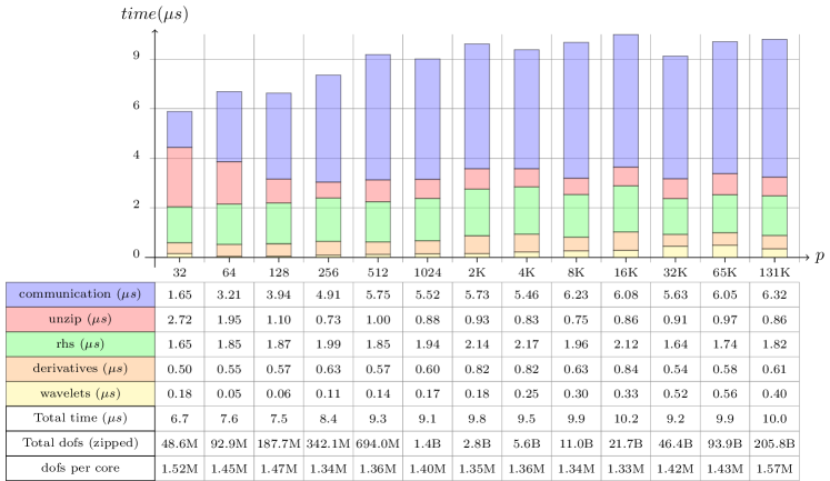
Scalability is a key requirement for large-scale codes such as Dendro. In the context of our target application this could be in order to run simulations of black hole mergers with large mass ratios, or to be able to run these simulations much faster. These cases correspond to weak and strong scaling respectively. As demonstrated in §4.3, Dendro-GR scales well in both cases. In this section, we demonstrate the ability of Dendro-GR  to scale to much larger core-counts for weak scaling. In Figure 13, we demonstrate weak scalability to $131,072$ cores on Titan using $1.5\times 10^{6}$ dofs/core for a largest problem of $206\times 10^{9}$ dofs. These correspond to a simulation of $q=10$, with increasing levels of refinement. There is a slight fluctuation in the number of unknowns per core at each problem size. Therefore, we report the average time for a single RK-step$/dof/p$. We can see that the average time per RK-step$/dof/p$ remains less than $10\mu s$. We note that the unzip costs are high at the lower core-counts and stabilize at higher core counts. This is due to a larger grain size at the smaller core-counts. The communication for a smaller number of processes is lower due to architectural reasons, as the majority of the communication happens primarily within the same node. This is common for most codes, and stabilizes for $p>512$ as the communication starts to get dominated by inter-node communication rather than intra-node communication.

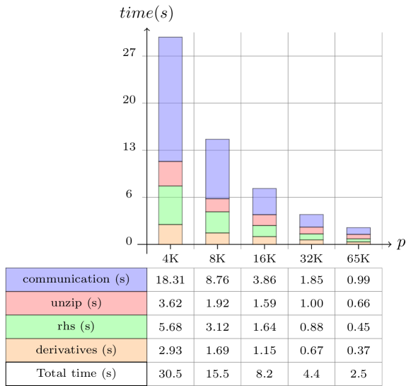
In Figure 14, we present the strong scaling results for Dendro-GR  to perform single RK step (i.e. averaged over 10 steps) for a fixed problem size of $10.5B$ unknowns in Titan  up to 4096 nodes. This experiment is carried out for a mass ratio of 10 binary merger problem with wavelet tolerance of $10^{-6}$. Note that for the strong scaling experiment we have disabled the re-mesh and inter-grid transfer operations in order to keep the problem size constant.

4.5 Large Mass Ratios

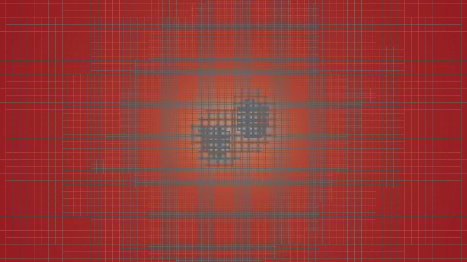
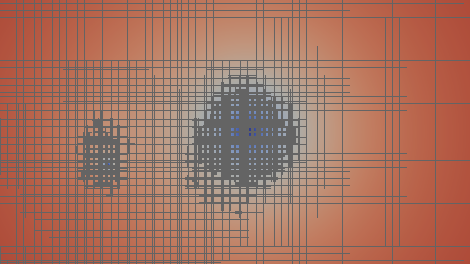
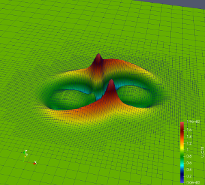
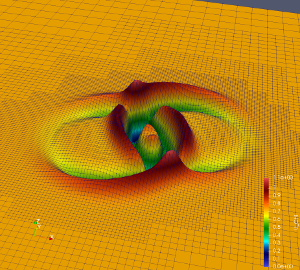
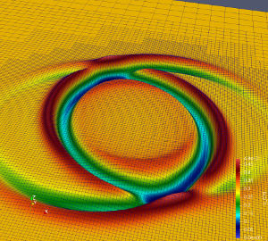
Finally, we present some representative images from simulations at mass rations of $q=1,10$, and $100$ in Figure 16. Here we plot the one of the evolved variables $\chi$ along with the adaptively refined mesh. We can observe the increased refinement needed to handle the increased mass ratio.

5 Conclusion

In this work we presented a high-adaptive and highly scalable framework for relatavistic simulations. By combining a parallel octree-refined adaptive mesh with wavelet adaptive multiresolution and a physics module to solve the Einstein equations of general relativity in the BSSNOK formulation, we were able to perform simulations of IMRIs of binary black holes with mass ratios on the order of 100:1. In designing our framework and methods, we have focused on ensuring portability and extensibility by the use of automatic code generation from symbolic notation. This enables portability, since new architectures can be supported by adding new generators rather than rewriting the application. The code is extensible as new applications can be created by using the symbolic interface without having to focus on writing scalable code. Since both of these are achieved using Python, this reduces the cost of extending and porting the framework, especially by non-specialist programmers. We also made improvements to fundamental algorithms required for generating octree-based meshes, specifically an improved 2:1 balancing algorithm and a scalable search algorithm fundamental to constructing meshing data-structures. Finally, we performed extensive comparisons with the current state-of-the-art codes and demonstrated excellent weak and strong scalability.

In the short time that LIGO and Virgo have been searching for gravitational waves, we have already learned exciting things about neutron stars [65, 80], the production of heavy elements (such as gold) [34], and the population of black holes in the universe [5]. The full scientific impact of multi-messenger astronomy is only realized when the observations are informed by sophisticated computer models of the underlying astrophysical phenomena. Dendro provides the ability to run these models in a scalable way, with local adaptivity criteria using WAMR. While AMR codes with block-adaptivity typically lose performance as the number of adaptive levels increases, Dendro achieves impressive scalability on a real application even with many levels of refinement. The combination of scalability and adaptivity will allow us to study the gravitational radiation from IMRIs without simplifying approximations in direct numerical simulations.

Appendix A Overview of BSSNOK  Equations

In this section, we briefly present the specific form of the BSSNOK equations used in this work. While a complete description of these equations can not be given here, many detailed descriptions can be found in the literature [46, 18, 79].

The spacetime metric is written using the ADM 3+1 decomposition

(1) $$ds^{2}=-\alpha^{2}\,dt^{2}+\gamma_{ij}\left(dx^{i}+\beta^{i}\,dt\right)\left(dx^{j}+\beta^{j}\,dt\right),$$

where $\alpha$ is the lapse function, $\beta^{i}$ is the shift vector, and $\gamma_{ij}$ is the 3-metric on a space-like hypersurface. We write $\gamma_{ij}$ in terms of a conformally flat metric $\tilde{\gamma}_{ij}$ and a conformal factor $\chi$ as

(2) $$\gamma_{ij}=\frac{1}{\chi}\tilde{\gamma}_{ij},\qquad\chi=\left(\det\gamma_{ij}\right)^{-1/3},\qquad\det\tilde{\gamma}_{ij}=1.$$

The extrinsic curvature $K_{ij}$ is decomposed into its trace $K$ and the conformal, trace-less extrinsic curvature $\tilde{A}_{ij}$

(3) $$K=K^{i}{}_{i},\qquad\tilde{A}_{ij}=\chi\left(K_{ij}-\frac{1}{3}\gamma_{ij}K\right).$$

Covariant derivatives on the hypersurface, $D_{i}$, use connection coefficients $\Gamma^{i}{}_{jk}$ computed with respect to $\gamma_{ij}$. Conformal connection coefficients, $\tilde{\Gamma}^{i}{}_{jk}$, are computed with respect to $\tilde{\gamma}_{ij}$, and the conformal connection functions are defined to be $\tilde{\Gamma}^{i}=\tilde{\gamma}^{jk}\tilde{\Gamma}^{i}{}_{ij}$.

Similar to the Maxwell equations in electromagnetism, the Einstein equations contain both hyperbolic and elliptic equations; the former are the evolution equations and the latter constraint equations. The vacuum BSSNOK evolution equations are

$$\partial_{t}\tilde{\gamma}_{ij} =\mathcal{L}_{\beta}\tilde{\gamma}_{ij}-2\alpha\tilde{A}_{ij}$$

$$\partial_{t}\chi =\mathcal{L}_{\beta}\chi+\frac{2}{3}\chi\left(\alpha K-\partial_{a}\beta^{a}\right)$$

$$\partial_{t}\tilde{A}_{ij} =\mathcal{L}_{\beta}\tilde{A}_{ij}+\chi\left(-D_{i}D_{j}\alpha+\alpha R_{ij}\right)^{TF}+\alpha\left(K\tilde{A}_{ij}-2\tilde{A}_{ik}\tilde{A}^{k}_{\,j}\right)$$

$$\partial_{t}K =\beta^{k}\partial_{k}K-D^{i}D_{i}\alpha+\alpha\left(\tilde{A}_{ij}\tilde{A}^{ij}+\frac{1}{3}K^{2}\right)$$

$$\partial_{t}\tilde{\Gamma}^{i} =\tilde{\gamma}^{jk}\partial_{j}\partial_{k}\beta^{i}+\frac{1}{3}\tilde{\gamma}^{ij}\partial_{j}\partial_{k}\beta^{k}+\beta^{j}\partial_{j}\tilde{\Gamma}^{i}-\tilde{\Gamma}^{j}\partial_{j}\beta^{i}+\frac{2}{3}\tilde{\Gamma}^{i}\partial_{j}\beta^{j}-2\tilde{A}^{ij}\partial_{j}\alpha$$

$$\quad+2\alpha\left(\tilde{\Gamma^{i}}_{jk}\tilde{A}^{jk}-\frac{3}{2\chi}\tilde{A}^{ij}\partial_{j}\chi-\frac{2}{3}\tilde{\gamma}^{ij}\partial_{j}K\right),$$

where $R_{ij}$ is the Ricci tensor on the hypersurface, $(\ldots)^{\rm TF}$ indicates the trace-free part of the quantity in parentheses, $\partial_{i}$ is the partial derivative with respect to $x^{i}$, and $\mathcal{L}_{\beta}$ is Lie derivative with respect to $\beta^{i}$. We use the “1+log” slicing condition and the $\Gamma$-driver shift condition to evolve the gauge (or coordinate) variables

$$\partial_{t}\alpha =\mathcal{L}_{\beta}\alpha-2\alpha K$$

$$\partial_{t}\beta^{i} =\lambda_{2}\beta^{j}\,\partial_{j}\beta^{i}+\frac{3}{4}f(\alpha)B^{i}$$

$$\partial_{t}B^{i} =\partial_{t}\tilde{\Gamma}^{i}-\eta B^{i}+\lambda_{3}\beta^{j}\,\partial_{j}B^{i}-\lambda_{4}\beta^{j}\,\partial_{j}\tilde{\Gamma}^{i},$$

where $f(\alpha)$ is an arbitrary function, and $\eta$ and $\{\lambda_{1},\lambda_{2},\lambda_{3},\lambda_{4}\}$ are parameters. We set $f(\alpha)=\lambda_{A}=1$ in this work.

The Hamiltonian and momentum constraints are elliptic equations that must be satisifed at all times during the evolution. These constraint equations in vacuum are

(4) $$R-K_{ij}K^{ij}+K^{2} =0$$

(5) $$D_{j}(K^{ij}-\gamma^{ij}K) =0.$$

We follow the common practice in numerical relativity by solving the Einstein equations in a “free evolution,” which means that the we evolve the the hyperbolic evolution equations for the BSSNOK variables and the gauge. The independent constraint equations are evaluated during the evolution to monitor the quality of the solution, but they are otherwise not used in the update.

A.1 NLSM: Non-linear Sigma Model

In this section, we introduce a simple model to demonstrate some capabilities of Dendro-GR, the classical wave equation. We can also add a nonlinear source to this equation to explore the Non-Linear Sigma Model with the hedgehog Ansatz (NLSM) [60]. We write the classical wave equation in a form similar to the the BSSNOK equations, i.e., with first derivatives in time and second derivatives in space. This allows us to test the Dendro-GR infrastructure for the more complicated BSSNOK equations.

The NLSM for a scalar function $\chi(t,x^{i})$ is the classical wave equation with a nonlinear source term. For simplicity we assume a flat spacetime and Cartesian coordinates $(t,x,y,z)$. The equation of motion is

(6) $$\frac{\partial^{2}\chi}{\partial t^{2}}-\left(\frac{\partial^{2}}{\partial x^{2}}+\frac{\partial^{2}}{\partial y^{2}}+\frac{\partial^{2}}{\partial z^{2}}\right)\chi=-\frac{\sin(2\chi)}{r^{2}},$$

where $r=\sqrt{x^{2}+y^{2}+z^{2}}$. We write the equation as a first order in time system by introducing the variable $\phi$ as

(7) $$\frac{\partial\chi}{\partial t} =\phi$$

(8) $$\frac{\partial\phi}{\partial t} =\left(\frac{\partial^{2}}{\partial x^{2}}+\frac{\partial^{2}}{\partial y^{2}}+\frac{\partial^{2}}{\partial z^{2}}\right)\chi-\frac{\sin(2\chi)}{r^{2}}.$$

We choose outgoing radiative boundary conditions for this system [18]. We assume that the variables $\chi$ and $\phi$ approach the form of spherical waves as $r\to\infty$, which decay as $1/r^{k}$. The radiative boundary conditions then have the form

(9) $$\frac{\partial f}{\partial t}=\frac{1}{r}\left(x\frac{\partial f}{\partial x}+y\frac{\partial f}{\partial y}+z\frac{\partial f}{\partial z}\right)-k(f-f_{0}),$$

where $f$ represents the functions $\chi$ and $\phi$, and $f_{0}$ is an asymptotic value. We assume $k=1$ for $\chi$ and $k=2$ for $\phi$.

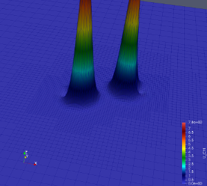
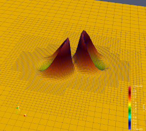
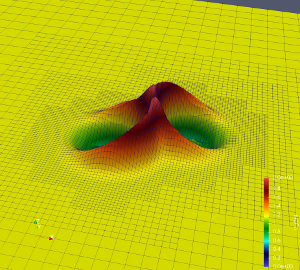
Using the Dendro-GR symbolic code generation framework we generate right-hand side evaluation for the equations 7 and 8 used in the time stepping scheme. Figure 17 shows frames from an evolution of the NLSM model using initial data from family (b) described in Table I of [60]. This test demonstrates that the Dendro-GR components for octree construction, mesh generation, spatial derivative operators, and time integration work accurately.

(a) step=0

(b) step=7

(c) step=11

(d) step=16

(e) step=23

(f) step=44

Figure 17: Frames from the evolution of the 3-dimensional NLSM that show the solution in the $z=0$ plane. The initial data are from family (b) defined in [60], which consist of two Gaussian functions for $\chi$ and velocities used to define $\phi$. Note how the mesh refines (based on the WAMR) as the pulses first interact nonlinearly at the center of the grid and then begin to propagate away from the origin.

Appendix B Code Evaluation and Verification

B.1 Getting and Compiling Dendro 

The Dendro simulation code is freely available at GitHub (https://github.com/paralab/Dendro-GR) under the MIT License. The latest version of the code can be obtained by cloning the repository

⬇

$ git clone git@github.com:paralab/Dendro-GR.git

The following dependencies are required to compile Dendro

• C/C++ compilers with C++11 standards and OpenMP support

• MPI implementation (e.g. openmpi, mvapich2 )

• ZLib compression library (used to write .vtu files in binary format with compression enabled)

• BLAS and LAPACK are optional and not needed for current version of Dendro

• CMake 2.8 or higher version

Note: We have tested the compilation and execution of Dendro with intel, gcc 4.8 or higher, openmpi, mpich2 and intelmpi and craympi (in Titan) using the linux operating systems.

To compile the code, execute these commands

⬇

$ cd <path to DENDRO directory >

$ mkdir build

$ cd build

$ ccmake ../

The following options for Dendro  can then be set in cmake:

• DENDRO_COMPUTE_CONSTRAINTS : Enables the computation of Hamiltonian and momentum constraints

• DENDRO_CONSEC_COMM_SELECT : If ON sub-communicators are selected from consecrative global ranks, otherwise sub-communicators are selected complete binary tree of global ranks (note that in this case global communicator size need to a power of 2).

• DENDRO_ENABLE_VTU_CONSTRAINT_OUT : Enables constraint variable output while time-stepping

• DENDRO_ENABLE_VTU_OUTPUT : Enables evolution variable output while time-stepping

• DENDRO_VTK_BINARY : If ON vtu files are written in binary format, else ASCII format (binary format recommended).

• DENDRO_VTK_ZLIB_COMPRES : If ON binary format is compressed (only effective if DENDRO_VTK_BINARY is ON)

• HILBERT_ORDERING : Hilbert SFC used if ON, otherwise Morton curve is used. (Hilbert curve is recommended to reduce the communication cost.)

• NUM_NPES_THRESHOLD : When running in large scale set this to $\sqrt{p}$ where $p$ number of mpi tasks for better performance.

• RK_SOLVER_OVERLAP_COMM_AND_COM : If ON non blocking communication is used and enable overlapping of communication and computation unzip (recommended option), otherwise blocking synchronized unzip is used.

After configuring Dendro, generate the Makefile (use c to configure and g to generate). Then execute make all to build all the targets. On completion, bssnSolver will be the main executable as related to this paper.

B.2 Getting Started: Running bssnSolver

bssnSolver  can be run as follows.

⬇

$ mpirun -np <number of mpi tasks>\

./bssnSolver \

<parameter file name>.par

Example parameter files can be found in BSSN_GR/pars/. The following is an example parameter file for equal mass ratio binary inspirals.

⬇

{

”DENDRO_VERSION”: 5.0,

”BSSN_RESTORE_SOLVER”:0,

”BSSN_IO_OUTPUT_FREQ”: 10,

”BSSN_REMESH_TEST_FREQ”: 5,

”BSSN_CHECKPT_FREQ”: 50,

”BSSN_VTU_FILE_PREFIX”: ”bssn_gr”,

”BSSN_CHKPT_FILE_PREFIX”: ”bssn_cp”,

”BSSN_PROFILE_FILE_PREFIX”: ”bssn_r1”,

”BSSN_DENDRO_GRAIN_SZ”: 100,

”BSSN_ASYNC_COMM_K”: 4,

”BSSN_DENDRO_AMR_FAC”: 1e0,

”BSSN_WAVELET_TOL”: 1e-4,

”BSSN_LOAD_IMB_TOL”: 1e-1,

”BSSN_RK_TIME_BEGIN”: 0,

”BSSN_RK_TIME_END”: 1000,

”BSSN_RK_TIME_STEP_SIZE”: 0.01,

”BSSN_DIM”: 3,

”BSSN_MAXDEPTH”: 12,

”ETA_CONST”: 2.0,

”ETA_R0”: 30.0,

”ETA_DAMPING”: 1.0,

”ETA_DAMPING_EXP”: 1.0,

”BSSN_LAMBDA”: {

”BSSN_LAMBDA_1”: 1,

”BSSN_LAMBDA_2”: 1,

”BSSN_LAMBDA_3”: 1,

”BSSN_LAMBDA_4”: 1

},

”BSSN_LAMBDA_F”: {

”BSSN_LAMBDA_F0”: 1.0,

”BSSN_LAMBDA_F1”: 0.0

},

”CHI_FLOOR”: 1e-4,

”BSSN_TRK0”: 0.0,

”KO_DISS_SIGMA”: 1e-1,

”BSSN_BH1”: {

”MASS”:0.48528137423856954,

”X”: 4.00000000e+00,

”Y”:0.0,

”Z”: 1.41421356e-05,

”V_X”: -0.00132697,

”V_Y”: 0.1123844,

”V_Z”: 0,

”SPIN”: 0,

”SPIN_THETA”:0,

”SPIN_PHI”: 0

},

”BSSN_BH2”: {

”MASS”:0.48528137423856954,

”X”:-4.00000000e+00,

”Y”:0.0,

”Z”:1.41421356e-05,

”V_X”: 0.00132697,

”V_Y”: -0.1123844,

”V_Z”: 0,

”SPIN”: 0,

”SPIN_THETA”:0,

”SPIN_PHI”: 0

}

}

Here we list the key options for bssnSolver with a short description.

• BSSN_RESTORE_SOLVER : Set $1$ to restore $RK$ solver from latest checkpoint.

• BSSN_IO_OUTPUT_FREQ : IO (i.e. vtu files) output frequency

• BSSN_CHECKPT_FREQ : Checkpoint file output frequency

• BSSN_REMESH_TEST_FREQ : Remesh test frequency (i.e. frequency in time steps that is being tested for re-meshing)

• BSSN_DENDRO_GRAIN_SZ : Number of octants per core

• BSSN_ASYNC_COMM_K : Number of variables that are being processed during an asynchronous unzip ($<24$)

• BSSN_DENDRO_AMR_FAC : Safety factor for coarsening i.e. coarsen if and only if $W_{c}\leq AMR\_FAC\times WAVELET\_TOL$ where $W_{c}$ is the computed wavelet coefficient.

• BSSN_WAVELET_TOL : Wavelet tolerance for WAMR.

• BSSN_MAXDEPTH : Maximum level of refinement allowed ($\leq 30$)

• KO_DISS_SIGMA : Kreiss-Oliger dissipation factor for BSSNOK formulation

• MASS : Mass of the black hole

• X : $x$ coordinate of the black hole

• Y : $y$ coordinate of the black hole

• Z : $z$ coordinate of the black hole

• V_X : momentum of the black hole in $x$ direction

• V_Y : momentum of the black hole in $y$ direction

• V_Z : momentum of the black hole in $z$ direction

• SPIN : magnitude of the spin of the black hole

• SPIN_THETA : magnitude of the spin of the black hole along $\theta$

• SPIN_PHI : magnitude of the spin of the black hole along $\phi$

B.2.1 Generating your own parameters

The intial data parameters for a binary black holes  [92] depend on the total mass ($M=m1+m2$), the mass ratio $q$ and the separation distance $d$. These parameters are calculated using the Python script BSSN_GR/scripts/id.py. The command to generate parameters for $q=10$, total mass $M=5$ and separation $d=16$ is

⬇

$ python3 id.py -M 5 -r 10 16

⬇

—————————————————————-

PUNCTURE PARAMETERS (par file foramt)

—————————————————————-

”BSSN_BH1”: {

”MASS”:4.489529,

”X”:1.454545,

”Y”:0.000000,

”Z”: 0.000014,

”V_X”: -0.020297,

”V_Y”: 0.423380,

”V_Z”: 0.000000,

”SPIN”: 0.000000,

”SPIN_THETA”:0.000000,

”SPIN_PHI”: 0.000000

},

”BSSN_BH2”: {

”MASS”:0.398620,

”X”:-14.545455,

”Y”:0.000000,

”Z”:0.000014,

”V_X”: 0.020297,

”V_Y”: -0.423380,

”V_Z”: 0.000000,

”SPIN”: 0.000000,

”SPIN_THETA”:0.000000,

”SPIN_PHI”: 0.000000

}

The tangential momentum is just an estimate, and the value for a

for a circular orbit is likely between (0.5472794147860968, 0.29947988193805547)

B.3 Symbolic interface and code generation

The BSSNOK formulation is a decomposition of the Einstein equations into 24 coupled hyperbolic PDEs. Writing the computation code for the BSSNOK formulation can be a tedious task. Hence we have written a symbolic Python interface to generate optimized C code to compute the BSSNOK equations. All the symbolic utilities necessary to write the BSSNOK formulation in symbolic Python can be found in GR/rhs_scripts/bssn/dendro.py and the symbolic BSSNOK code can be found in GR/rhs_scripts/bssn/bssn.py. This could be modified for more advanced uses of the code such as including new equations to describe additional physics or for introducing a different formulation of the Einstein equations.

B.4 Profiling the code

Dendro contains built-in profiler code which enables one to profile the code extensively. On configuration, a user can enable/disable the internal profiling flags using ENABLE_DENDRO_PROFILE_COUNTERS and the profile output can be changed between a human readable version and a tab separated format using the flag BSSN_PROFILE_HUMAN_READABLE. Note that in order to profile communication, internal profile flags need to be enabled. The following is an example of profiling output for the first 10 time steps.

⬇

active npes : 16

global npes : 16

current step : 10

partition tol : 0.1

wavelet tol : 0.0001

maxdepth : 12

Elements : 4656

DOF(zip) : 279521

DOF(unzip) : 2078609

============ MESH =================

step min(#) mean(#) max(#)

ghost Elements 634 824.062 1065

local Elements 263 291 319

ghost Nodes 43781 55671.7 71693

local Nodes 14292 17470.1 20705

send Nodes 18760 24872.9 36861

recv Nodes 18113 24872.9 33777

========== RUNTIME =================

step min(s) mean(s) max(s)

++2:1 balance 0 0 0

++mesh 1.9753 1.98299 1.98946

++rkstep 20.159 20.1856 20.1996

++ghostExchge. 1.81442 3.15703 4.49568

++unzip_sync 8.27839 9.67293 11.0991

++unzip_async 0 0 0

++isReMesh 0.04642 0.117357 0.207305

++gridTransfer 1.53709 1.54899 1.56531

++deriv 1.98942 2.34851 2.76695

++compute_rhs 4.00119 4.61547 5.11566

–compute_rhs_a 0.0137962 0.0245449 0.0351532

–compute_rhs_b 0.0296426 0.0503471 0.069537

–compute_rhs_gt 0.111898 0.12846 0.15463

–compute_rhs_chi 0.0170642 0.0315392 0.044856

–compute_rhs_At 2.40738 2.72922 3.05622

–compute_rhs_K 0.358215 0.39879 0.457139

–compute_rhs_Gt 0.774211 0.933581 1.05702

–compute_rhs_B 0.0575426 0.071209 0.0855094

++boundary con 0 0.0421986 0.134712

++zip 0.23529 0.260862 0.291513

++vtu 0.0872362 0.101362 0.128246

++checkpoint 3.27e-06 3.85e-06 5.7469e-06

B.5 Visualizing the data

Dendro  can be configured to output parallel unstructured grid files in binary file format (.pvtu). These files can be visualized using any visualization tool which supports VTK file formats. All the images presented in this paper used Paraview due to its robustness and scalability. Paraview allows Python based scripting to perform pvbatch visualization, an example pvpython script can be found in scripts/bssnVis.py

B.6 BSSNOK: Verification Tests

In this section, we present experimental evaluations that we performed to ensure the accuracy of the simulation code.

B.7 Accuracy of stencil operators

In order to test the accuracy and convergence of WAMR and the derivative stencils, we used a known function to generate adaptive octree grid based on the wavelet expansion. Then we compute numerical derivatives using finite difference stencils which are compared against the analytical derivatives of $f(x,y,z)$. $l_{2}$ and $l_{\infty}$ norms of the comparison is given in the Table 3.

derivative	grid points	$\left\lVert.\right\rVert_{2}$	$\left\lVert.\right\rVert_{\infty}$
$\partial_{x}$	4913	0.0201773	0.00144632
$\partial_{x}$	99221	0.000849063	2.74672e-05

Table 3: Normed difference in numerical derivative and analytical derivative evaluated at grid points for the function $f(x,y,z)=sin(2\pi x)sin(2\pi y)sin(2\pi z))$where in both cases wavelet tolerance of $10^{-8}$ but increasing maximum level of refinement (i.e. maxDepth) from $4$ to $6$. Note that when maxDepth increases number of grid points increase hence normed difference between numerical and analytical derivatives goes down significantly.

B.8 Accuracy of symbolic interface and code generation

Given the complexity of the BSSNOK equations, writing code to evaluate these equations can be an error-prone and tedious task. For example, to evaluate the equations we need to calculate more than 300 finite derivatives. Hence Dendro provides a symbolic framework written in SymPy for automatically generating C++ code for the equations. The user writes equations in a high-level representation that more closely resembles their symbolic form. We can then use the computational graph of the equations to generate optimized C++ code. The accuracy of the symbolic framework and code generation is certified by comparing results from the generated C++ code to those from the HAD code, an established and tested code for numerical relativity.

This table shows a comparison of BSSNOK equations (i.e. all 24 equations), evaluated over a grid of $128^{3}$ points by arbitrary, non-zero functions by both the Dendro and HAD codes. All spatial derivatives in the equations are evaluated using finite differences, for both the Dendro and HAD codes. The table reports the $L_{2}$ norm of the difference in the equations as evaluated in both codes, as well as the $L_{2}$ norms of the functions used to evaluate the equations. Equations with residual norms of order $10^{-15}$ are clearly at machine zero, but this low level is reached for only the simplest equations. Residuals with norms of order $10^{-12}$ arise in complicated equations, where finite precision errors can accumulate in hundreds of floating point operations. The optimized equations require about 4500 floating point operations to evaluate at a single point.

⬇

L2 Norms differences in the HAD and DENDRO equations on 128^3 points.

————————————————————————

|| diff 0 || = 1.18413e-15, || rhs HAD || = 1.28114, || rhs DENDRO || = 1.28114

|| diff 1 || = 7.53412e-16, || rhs HAD || = 2.18877, || rhs DENDRO || = 2.18877

|| diff 2 || = 4.98271e-16, || rhs HAD || = 1.66315, || rhs DENDRO || = 1.66315

|| diff 3 || = 1.03346e-15, || rhs HAD || = 0.720477,|| rhs DENDRO || = 0.720477

|| diff 4 || = 5.82489e-16, || rhs HAD || = 1.40142, || rhs DENDRO || = 1.40142

|| diff 5 || = 4.93128e-16, || rhs HAD || = 0.797567,|| rhs DENDRO || = 0.797567

|| diff 6 || = 1.94194e-11, || rhs HAD || = 19.0107, || rhs DENDRO || = 19.0107

|| diff 7 || = 2.14958e-11, || rhs HAD || = 19.5221, || rhs DENDRO || = 19.5221

|| diff 8 || = 4.0673e-12, || rhs HAD || = 8.96364, || rhs DENDRO || = 8.96364

|| diff 9 || = 1.58532e-11, || rhs HAD || = 10.1459, || rhs DENDRO || = 10.1459

|| diff 10 || = 4.31184e-12, || rhs HAD || = 8.70053, || rhs DENDRO || = 8.70053

|| diff 11 || = 4.95696e-12, || rhs HAD || = 10.8644, || rhs DENDRO || = 10.8644

|| diff 12 || = 4.27211e-15, || rhs HAD || = 19.3546, || rhs DENDRO || = 19.3546

|| diff 13 || = 2.29542e-10, || rhs HAD || = 93.4829, || rhs DENDRO || = 93.4829

|| diff 14 || = 1.7484e-11, || rhs HAD || = 40.0804, || rhs DENDRO || = 40.0804

|| diff 15 || = 4.79216e-11, || rhs HAD || = 30.9279, || rhs DENDRO || = 30.9279

|| diff 16 || = 2.03434e-11, || rhs HAD || = 26.0603, || rhs DENDRO || = 26.0603

|| diff 17 || = 1.07479e-15, || rhs HAD || = 15.5765, || rhs DENDRO || = 15.5765

|| diff 18 || = 3.00151e-15, || rhs HAD || = 32.9891, || rhs DENDRO || = 32.9891

|| diff 19 || = 7.79103e-16, || rhs HAD || = 8.10107, || rhs DENDRO || = 8.10107

|| diff 20 || = 7.77113e-16, || rhs HAD || = 9.01369, || rhs DENDRO || = 9.01369

|| diff 21 || = 1.74839e-11, || rhs HAD || = 46.3141, || rhs DENDRO || = 46.3141

|| diff 22 || = 4.79217e-11, || rhs HAD || = 32.7981, || rhs DENDRO || = 32.7981

|| diff 23 || = 2.03434e-11, || rhs HAD || = 32.7256, || rhs DENDRO || = 32.7256

B.9 Single black hole

Prior to simulating binary inspirals, we perform simple experiments with a single black hole to ensure the accuracy of the simulation code. While a single black hole is a stable, static solution of the Einstein equations, although there is some transient time dependence with:w our particular coordinate conditions. The black hole parameters (parameter file can be found in SC18_AE/par/single_bh1.par in the repository) for this test is given below. Note that to generate initial data for a single black hole, we place one of the black holes in the binary far from the computational domain and set its mass to zero.

⬇

”BSSN_BH1”: { ”MASS”:1.0, ”X”:0.0, ”Y”:0.0,

”Z”: 0.00123e-6, ”V_X”: 0.0, ”V_Y”: 0.0,

”V_Z”: 0.0, ”SPIN”: 0,

”SPIN_THETA”:0, ”SPIN_PHI”: 0 },

”BSSN_BH2”: { ”MASS”:1e-15,”X”:1e15, ”Y”:0.0,

”Z”:0.00123e-6, ”V_X”: 0.0, ”V_Y”: 0.0,

”V_Z”: 0.0, ”SPIN”: 0,

”SPIN_THETA”:0, ”SPIN_PHI”: 0 }

B.10 Boosted Single Black Hole

The next experiment is an extension of the single BH test; it “boosts” the BH with constant velocity in $x$-direction. The constant velocity of the BH should be apparent in the evolution. The parameter file for this test can be found in the repository at SC18_AE/par/single_bh1_boost.par. The black hole parameters are given below (note that $BSSN\_BH1$ has a momentum of 0.114 in $x$-direction).

⬇

”BSSN_BH1”: { ”MASS”:1.0, ”X”:0.0, ”Y”:0.0,

”Z”: 0.00123e-6, ”V_X”: 0.114, ”V_Y”: 0.0,

”V_Z”: 0.0, ”SPIN”: 0,

”SPIN_THETA”:0, ”SPIN_PHI”: 0 },

”BSSN_BH2”: { ”MASS”:1e-15,”X”:1e15, ”Y”:0.0,

”Z”:0.00123e-6, ”V_X”: 0.0, ”V_Y”: 0.0,

”V_Z”: 0.0, ”SPIN”: 0,

”SPIN_THETA”:0, ”SPIN_PHI”: 0 }

(a) $\SS=0,\ {\rm time}=0~{}M$

(b) $\SS=500,\ {\rm time}=21.97~{}M$

(c) $\SS=1000,\ {\rm time}=43.94~{}M$

(d) $\SS=1500,\ {\rm time}=65.91~{}M$

(e) $\SS=2000,\ {\rm time}=87.88~{}M$

(f) $\SS=2500,\ {\rm time}=109.85~{}M$

(g) $\SS=3000,\ {\rm time}=131.82~{}M$

(h) $\SS=3500,\ {\rm time}=153.79~{}M$

(i) $\SS=4000,\ {\rm time}=175.76~{}M$

(j) $\SS=4500,\ {\rm time}=197.73~{}M$

(k) $\SS=5000,\ {\rm time}=219.70~{}M$

(l) $\SS=5500,\ {\rm time}=241.67~{}M$

(m) $\SS=6000,\ {\rm time}=263.64~{}M$

(n) $\SS=6500,\ {\rm time}=285.61~{}M$

Figure 18: A single black hole boosted in the $x$-direction, with maxdepth=12 and wavelet tolerance of $10^{-3}$. Time is given in terms of the black hole mass, $M$.

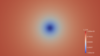
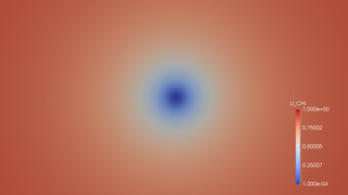
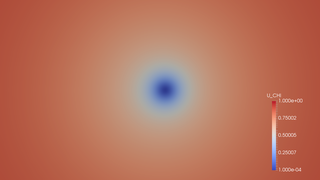
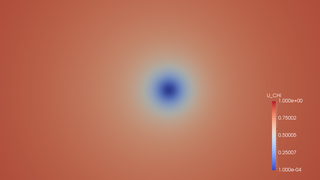
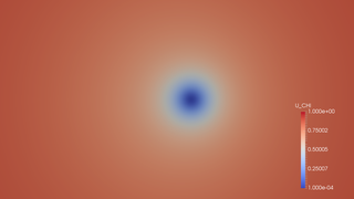
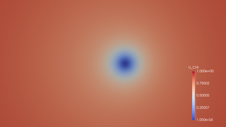
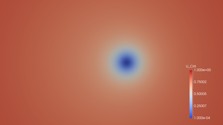
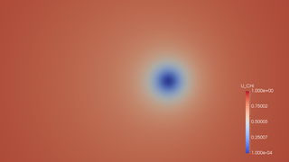
B.11 Constraint equations

Similar to the Maxwell equations of electrodynamics, the Einstein equations contain both hyperbolic evolution equations and elliptic constraint equations, which must be satisfied at all times. Following the common practice in numerical relativity, we evolve the hyperbolic equations and monitor the quality of the solution by checking that the constraint equations are satisfied. The choice of coordinates for the BBH evolution (the puncture gauge) does induce constraint violations in the vicinity of each black hole. The violations of the constraint equations in our runs are consistent with the discretization error expected for the numerical derivatives in the constraint equations and the constraint violations near the black holes (punctures). An example of monitored constraint violations are listed in the Table 4.

Time (M)	$\left\lVert\mathcal{H}_{r>a}\right\rVert_{2}$	$\left\lVert M1_{r>a}\right\rVert_{2}$	$\left\lVert M2_{r>a}\right\rVert_{2}$	$\left\lVert M3_{r>a}\right\rVert_{2}$
0	0.000777861	1.01855e-05	1.23443e-05	7.17572e-06
0.976562	0.000808294	3.05681e-05	2.91217e-05	2.79631e-05
1.95312	0.000793783	5.03912e-05	3.93872e-05	4.06693e-05
2.92969	0.00079551	7.54643e-05	5.068e-05	5.42466e-05
3.90625	0.000956987	0.000102901	7.38208e-05	7.47156e-05
4.88281	0.00247348	0.000200055	0.000140583	0.000139008

Table 4: Violation of constraint equations with time for an equal mass ratio binary merger simulation done using OT. Note that $\mathcal{H}$, $M1,M2,M3$ denotes the Hamiltonian and 3 momentum component constraints that is being monitored through the evolution.

B.12 Binary black holes with mass ratio $q=1$

We performed a series of short-term binary BH evolutions with different mass ratios. This run was used to validate the code by comparing the trajectories of the BHs calculated using Dendro to the trajectories calculated by HAD. Frames from the evolution are shown in the Figure 20, and the BH parameters used for this run are listed below.

⬇

”BSSN_BH1”: {

”MASS”:0.485,

”X”: 4.00e+00, ”Y”:0.0, ”Z”: 1.41-05,

”V_X”: -0.00133, ”V_Y”: 0.112, ”V_Z”: 0,

”SPIN”: 0, ”SPIN_THETA”:0, ”SPIN_PHI”: 0 },

”BSSN_BH2”: {

”MASS”:0.485,

”X”:-4.00+00, ”Y”:0.0, ”Z”:1.41-05,

”V_X”: 0.00132, ”V_Y”: -0.112, ”V_Z”: 0,

”SPIN”: 0, ”SPIN_THETA”:0, ”SPIN_PHI”: 0 }

Figure 19: $l_{2}$ norm of the Hamiltonian and momentum constraint violation as hyperbolic equations are evolved in time for equal mass ratio binary black hole configuration test run performed using Dendro-GR. Note that the final spike in constraint violation is happens during the merging even of binary black holes.

(a) $\SS=0,\ {\rm time}=0~{}M$

(b) $\SS=500,\ {\rm time}=21.97~{}M$

(c) $\SS=1000,\ {\rm time}=43.94~{}M$

(d) $\SS=1500,\ {\rm time}=65.91~{}M$

(e) $\SS=2000,\ {\rm time}=87.88~{}M$

(f) $\SS=2500,\ {\rm time}=109.85~{}M$

(g) $\SS=3000,\ {\rm time}=131.82~{}M$

(h) $\SS=3500,\ {\rm time}=153.79~{}M$

(i) $\SS=4000,\ {\rm time}=175.76~{}M$

(j) $\SS=4500,\ {\rm time}=197.73~{}M$

(k) $\SS=5000,\ {\rm time}=219.70~{}M$

(l) $\SS=5500,\ {\rm time}=241.67~{}M$

Figure 20: This figure shows frames from the evolution of a black hole binary with an equal mass ratio, $q=1$. Time is measured in terms of the total black hole mass $M$.

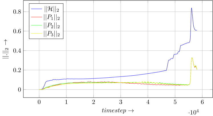
B.13 Binary black holes with mass ratio $q=10$

We performed a short simulation with a mass ratio $q=10$ This is a short demonstration run to show that Dendro easily handles large mass ratios and gives consistent results for the binary evolution. Frames from the evolution are shown in figure, and the BH parameters used for this run are listed below.

⬇

”BSSN_BH1”: {

”MASS”:0.903,

”X”:5.45-01, ”Y”:0.0, ”Z”: 1.41-05,

”V_X”: -3.90e-04, ”V_Y”: 0.0470, ”V_Z”: 0,

”SPIN”: 0, ”SPIN_THETA”:0, ”SPIN_PHI”: 0 },

”BSSN_BH2”: {

”MASS”:0.0845,

”X”:-5.45+00, ”Y”:0.0, ”Z”:1.41-05,

”V_X”: 3.90e-04, ”V_Y”: -0.0470, ”V_Z”: 0,

”SPIN”: 0, ”SPIN_THETA”:0, ”SPIN_PHI”: 0 }

(a) $\SS=0,\ {\rm time}=0~{}M$

(b) $\SS=500,\ {\rm time}=21.97~{}M$

(c) $\SS=1000,\ {\rm time}=43.94~{}M$

(d) $\SS=1500,\ {\rm time}=65.91~{}M$

(e) $\SS=2000,\ {\rm time}=87.88~{}M$

(f) $\SS=2500,\ {\rm time}=109.85~{}M$

(g) $\SS=3000,\ {\rm time}=131.82~{}M$

(h) $\SS=3500,\ {\rm time}=153.79~{}M$

(i) $\SS=4000,\ {\rm time}=175.76~{}M$

(j) $\SS=4500,\ {\rm time}=197.73~{}M$

(k) $\SS=5000,\ {\rm time}=219.70~{}M$

(l) $\SS=5500,\ {\rm time}=241.67~{}M$

Figure 21: This figure shows frames from the evolution of a black hole binary with mass ratio $q=10$. Time is measured in terms of the total black hole mass $M$.

B.14 Binary black holes with mass ratio $q=100$

We performed a short simulation with a mass ratio $q=100$ This is a short demonstration run to show that Dendro produces the proper grid structure for this system and reasonable results for a very challenging binary configuration. Frames from the evolution are shown in the figure and the BH parameters used for this run are listed below.

⬇

”BSSN_BH1”: {

”MASS”:0.989,

”X”:5.94-02, ”Y”:0.0, ”Z”: 1.41-05,

”V_X”: -5.60-06, ”V_Y”: 5.61-03, ”V_Z”: 0,

”SPIN”: 0, ”SPIN_THETA”:0, ”SPIN_PHI”: 0 },

”BSSN_BH2”: {

”MASS”:0.00914,

”X”:-5.94+00, ”Y”:0.0, ”Z”:1.41421356e-05,

”V_X”: 5.60-06, ”V_Y”: -5.61-03, ”V_Z”: 0,

”SPIN”: 0, ”SPIN_THETA”:0, ”SPIN_PHI”: 0 }

(a) $\SS=0,\ {\rm time}=0~{}M$

(b) $\SS=500,\ {\rm time}=21.97~{}M$

(c) $\SS=1000,\ {\rm time}=43.94~{}M$

(d) $\SS=1500,\ {\rm time}=65.91~{}M$

(e) $\SS=2000,\ {\rm time}=87.88~{}M$

(f) $\SS=2500,\ {\rm time}=109.85~{}M$

(g) $\SS=3000,\ {\rm time}=131.82~{}M$

(h) $\SS=3500,\ {\rm time}=153.79~{}M$

(i) $\SS=4000,\ {\rm time}=175.76~{}M$

(j) $\SS=4500,\ {\rm time}=197.73~{}M$

(k) $\SS=5000,\ {\rm time}=219.70~{}M$

(l) $\SS=5500,\ {\rm time}=241.67~{}M$

Figure 22: This figure shows frames from the evolution of a black hole binary with mass ratio $q=100$. Time is given in terms of the total mass $M$.

References

- [1] LIGO home page. http://flash.uchicago.edu/website/home/, 2018.
- [2] Virgo home page. http://http://www.virgo-gw.eu, 2018.
- [3] J. Abadie et al., Predictions for the Rates of Compact Binary Coalescences Observable by Ground-based Gravitational-wave Detectors, Class.Quant.Grav., 27 (2010), p. 173001, https://doi.org/10.1088/0264-9381/27/17/173001, https://arxiv.org/abs/1003.2480.
- [4] B. Abbott et al., GW170817: Observation of Gravitational Waves from a Binary Neutron Star Inspiral, Phys. Rev. Lett., 119 (2017), p. 161101, https://doi.org/10.1103/PhysRevLett.119.161101, https://arxiv.org/abs/1710.05832.
- [5] B. P. Abbott et al., Astrophysical Implications of the Binary Black-Hole Merger GW150914, Astrophys. J., 818 (2016), p. L22, https://doi.org/10.3847/2041-8205/818/2/L22, https://arxiv.org/abs/1602.03846.
- [6] B. P. Abbott et al., GW151226: Observation of gravitational waves from a 22-solar-mass binary black hole coalescence, Phys. Rev. Lett., 116 (2016), p. 241103, https://doi.org/10.1103/PhysRevLett.116.241103, http://link.aps.org/doi/10.1103/PhysRevLett.116.241103.
- [7] B. P. Abbott et al., Observation of Gravitational Waves from a Binary Black Hole Merger, Phys. Rev. Lett., 116 (2016), p. 061102, https://doi.org/10.1103/PhysRevLett.116.061102, https://arxiv.org/abs/1602.03837.
- [8] B. P. Abbott et al., Observation of gravitational waves from a binary black hole merger, Phys. Rev. Lett., 116 (2016), p. 061102, https://doi.org/10.1103/PhysRevLett.116.061102, http://link.aps.org/doi/10.1103/PhysRevLett.116.061102.
- [9] B. P. Abbott et al., Estimating the Contribution of Dynamical Ejecta in the Kilonova Associated with GW170817, Astrophys. J., 850 (2017), p. L39, https://doi.org/10.3847/2041-8213/aa9478, https://arxiv.org/abs/1710.05836.
- [10] B. P. Abbott et al., Gravitational Waves and Gamma-rays from a Binary Neutron Star Merger: GW170817 and GRB 170817A, Astrophys. J., 848 (2017), p. L13, https://doi.org/10.3847/2041-8213/aa920c, https://arxiv.org/abs/1710.05834.
- [11] B. P. Abbott et al., GW170104: Observation of a 50-Solar-Mass Binary Black Hole Coalescence at Redshift 0.2, Phys. Rev. Lett., 118 (2017), p. 221101, https://doi.org/10.1103/PhysRevLett.118.221101, https://arxiv.org/abs/1706.01812.
- [12] B. P. Abbott et al., GW170814: A Three-Detector Observation of Gravitational Waves from a Binary Black Hole Coalescence, Phys. Rev. Lett., 119 (2017), p. 141101, https://doi.org/10.1103/PhysRevLett.119.141101, https://arxiv.org/abs/1709.09660.
- [13] B. P. Abbott et al., Multi-messenger Observations of a Binary Neutron Star Merger, Astrophys. J., 848 (2017), p. L12, https://doi.org/10.3847/2041-8213/aa91c9, https://arxiv.org/abs/1710.05833.
- [14] F. Acernese et al., Advanced Virgo: a second-generation interferometric gravitational wave detector, Class. Quant. Grav., 32 (2015), p. 024001, https://doi.org/10.1088/0264-9381/32/2/024001, https://arxiv.org/abs/1408.3978.
- [15] A. Ahimian, I. Lashuk, S. Veerapaneni, C. Aparna, D. Malhotra, I. Moon, R. Sampath, A. Shringarpure, J. Vetter, R. Vuduc, D. Zorin, and G. Biros, Petascale direct numerical simulation of blood flow on 200k cores and heterogeneous architectures, in SC10: Proceedings of the International Conference for High Performance Computing, Networking, Storage, and Analysis, ACM/IEEE, 2010. (Gordon Bell Prize).
- [16] A. Akansu and R. Haddad, Academic Press, 1992.
- [17] A. Albert et al., Search for High-energy Neutrinos from Binary Neutron Star Merger GW170817 with ANTARES, IceCube, and the Pierre Auger Observatory, Astrophys. J., 850 (2017), p. L35, https://doi.org/10.3847/2041-8213/aa9aed, https://arxiv.org/abs/1710.05839.
- [18] M. Alcubierre, Introduction to 3+1 numerical relativity, International series of monographs on physics, Oxford Univ. Press, Oxford, 2008.
- [19] L. B. N. L. Applied Numerical Algorithms Group, Chombo –infrastructure for adaptive mesh refinement. http://seesar.lbl.gov/anag/chombo/, 2006.
- [20] S. Babak, A. Taracchini, and A. Buonanno, Validating the effective-one-body model of spinning, precessing binary black holes against numerical relativity, (2016), https://arxiv.org/abs/1607.05661.
- [21] T. W. Baumgarte and S. L. Shapiro, On the numerical integration of Einstein’s field equations, Phys.Rev., D59 (1999), p. 024007, https://doi.org/10.1103/PhysRevD.59.024007, https://arxiv.org/abs/gr-qc/9810065.
- [22] J. Bédorf, E. Gaburov, and S. Portegies Zwart, Bonsai: A GPU Tree-Code, in Advances in Computational Astrophysics: Methods, Tools, and Outcome, R. Capuzzo-Dolcetta, M. Limongi, and A. Tornambè, eds., vol. 453 of Astronomical Society of the Pacific Conference Series, July 2012, p. 325, https://arxiv.org/abs/1204.2280.
- [23] M. Bern, D. Eppstein, and S.-H. Teng, Parallel construction of quadtrees and quality triangulations, International Journal of Computational Geometry & Applications, 9 (1999), pp. 517–532.
- [24] S. Bertoluzza and G. Naldi, A wavelet collocation method for the numerical solution of partial differnetial equations, Appl. Comput. Harmon. A., 3 (1996), pp. 1–9.
- [25] M. Boyle, Transformations of asymptotic gravitational-wave data, Phys. Rev. D, 93 (2016), p. 084031, https://doi.org/10.1103/PhysRevD.93.084031, https://link.aps.org/doi/10.1103/PhysRevD.93.084031.
- [26] B. Bruegmann, J. A. Gonzalez, M. Hannam, S. Husa, U. Sperhake, and W. Tichy, Calibration of Moving Puncture Simulations, Phys. Rev., D77 (2008), p. 024027, https://doi.org/10.1103/PhysRevD.77.024027, https://arxiv.org/abs/gr-qc/0610128.
- [27] M. Bugner, T. Dietrich, S. Bernuzzi, A. Weyhausen, and B. Bruegmann, Solving 3D relativistic hydrodynamical problems with WENO discontinuous Galerkin methods, (2015), https://arxiv.org/abs/1508.07147.
- [28] C. Burstedde, L. C. Wilcox, and O. Ghattas, p4est: Scalable algorithms for parallel adaptive mesh refinement on forests of octrees, SIAM Journal on Scientific Computing, 33 (2011), pp. 1103–1133, https://doi.org/10.1137/100791634.
- [29] Cactus Computational Toolkit. http://www.cactuscode.org.
- [30] M. Campanelli, C. O. Lousto, P. Marronetti, and Y. Zlochower, Accurate evolutions of orbiting black-hole binaries without excision, Phys. Rev. Lett., 96 (2006), p. 111101, https://arxiv.org/abs/gr-qc/0511048.
- [31] Carpet, an AMR driver for Cactus. http://www.carpetcode.org.
- [32] J. Cocke, Global common subexpression elimination, in Proceedings of a Symposium on Compiler Optimization, New York, NY, USA, 1970, ACM, pp. 20–24, https://doi.org/10.1145/800028.808480, http://doi.acm.org/10.1145/800028.808480.
- [33] R. Courant, K. Friedrichs, and H. Lewy, On the partial difference equations of mathematical physics, IBM Journal of Research and Development, 11 (1967), pp. 215–234, https://doi.org/10.1147/rd.112.0215.
- [34] B. Côté, C. L. Fryer, K. Belczynski, O. Korobkin, M. Chruslinska, N. Vassh, M. R. Mumpower, J. Lippuner, T. M. Sprouse, R. Surman, and R. Wollaeger, The origin of r -process elements in the milky way, The Astrophysical Journal, 855 (2018), p. 99, http://stacks.iop.org/0004-637X/855/i=2/a=99.
- [35] J. DeBuhr, B. Zhang, M. Anderson, D. Neilsen, and E. W. Hirschmann, Relativistic Hydrodynamics with Wavelets, (2015), https://arxiv.org/abs/1512.00386.
- [36] D. L. Donoho, Interpolating wavelet transforms, Technical Report, Department of Statistics, Stanford University, 2 (1992).
- [37] M. Dumbser, F. Guercilena, S. Koeppel, L. Rezzolla, and O. Zanotti, A strongly hyperbolic first-order CCZ4 formulation of the Einstein equations and its solution with discontinuous Galerkin schemes, (2017), https://arxiv.org/abs/1707.09910.
- [38] Einstein Toolkit. http://einsteintoolkit.org.
- [39] Z. B. Etienne, V. Paschalidis, R. Haas, P. Mösta, and S. L. Shapiro, IllinoisGRMHD: An Open-Source, User-Friendly GRMHD Code for Dynamical Spacetimes, Class. Quant. Grav., 32 (2015), p. 175009, https://doi.org/10.1088/0264-9381/32/17/175009, https://arxiv.org/abs/1501.07276.
- [40] E. Evans, S. Iyer, E. Schnetter, W.-M. Suen, J. Tao, R. Wolfmeyer, and H.-M. Zhang, Computational relativistic astrophysics with adaptive mesh refinement: Testbeds, Phys. Rev. D, 71 (2005), p. 081301, https://doi.org/10.1103/PhysRevD.71.081301, https://link.aps.org/doi/10.1103/PhysRevD.71.081301.
- [41] M. Fernando, D. Duplyakin, and H. Sundar, Machine and application aware partitioning for adaptive mesh refinement applications, in Proceedings of the 26th International Symposium on High-Performance Parallel and Distributed Computing, HPDC ’17, New York, NY, USA, 2017, ACM, pp. 231–242, https://doi.org/10.1145/3078597.3078610, http://doi.acm.org/10.1145/3078597.3078610.
- [42] W. D. Frazer and A. C. McKellar, Samplesort: A sampling approach to minimal storage tree sorting, J. ACM, 17 (1970), pp. 496–507, https://doi.org/10.1145/321592.321600, http://doi.acm.org/10.1145/321592.321600.
- [43] J. M. Fregeau, S. L. Larson, M. C. Miller, R. W. O’Shaughnessy, and F. A. Rasio, Observing IMBH-IMBH Binary Coalescences via Gravitational Radiation, Astrophys. J., 646 (2006), pp. L135–L138, https://doi.org/10.1086/507106, https://arxiv.org/abs/astro-ph/0605732.
- [44] A. Goldstein et al., An Ordinary Short Gamma-Ray Burst with Extraordinary Implications: Fermi-GBM Detection of GRB 170817A, Astrophys. J., 848 (2017), p. L14, https://doi.org/10.3847/2041-8213/aa8f41, https://arxiv.org/abs/1710.05446.
- [45] T. Goodale, G. Allen, G. Lanfermann, J. Masso, T. Radke, E. Seidel, and J. Shalf, The cactus framework and toolkit: Design and applications, in Vector and Parallel Processing - VECPAR ’2002, 5th International Conference, Springer, 2003, http://www.springerlink.com/content/2fapcbeyyc1xg0mm/.
- [46] E. Gourgoulhon, 3+1 Formalism and Bases of Numerical Relativity, ArXiv General Relativity and Quantum Cosmology e-prints, (2007), https://arxiv.org/abs/gr-qc/0703035.
- [47] P. B. Graff, A. Buonanno, and B. S. Sathyaprakash, Missing Link: Bayesian detection and measurement of intermediate-mass black-hole binaries, Phys. Rev., D92 (2015), p. 022002, https://doi.org/10.1103/PhysRevD.92.022002, https://arxiv.org/abs/1504.04766.
- [48] J. Healy, C. O. Lousto, Y. Zlochower, and M. Campanelli, The rit binary black hole simulations catalog, Classical and Quantum Gravity, 34 (2017), p. 224001, http://stacks.iop.org/0264-9381/34/i=22/a=224001.
- [49] M. Holmström, Solving hyperbolic pdes using interpolating wavelets, SIAM J. Sci. Comput., 21 (1999), pp. 405–420.
- [50] S. Husa, I. Hinder, and C. Lechner, Kranc: A Mathematica application to generate numerical codes for tensorial evolution equations, Comput. Phys. Commun., 174 (2006), pp. 983–1004, https://doi.org/10.1016/j.cpc.2006.02.002, https://arxiv.org/abs/gr-qc/0404023.
- [51] M. F. Ionescu and K. E. Schauser, Optimizing parallel bitonic sort, in Proceedings 11th International Parallel Processing Symposium, April 1997, pp. 303–309, https://doi.org/10.1109/IPPS.1997.580914.
- [52] K. Jani, J. Healy, J. A. Clark, L. London, P. Laguna, and D. Shoemaker, Georgia tech catalog of gravitational waveforms, Classical and Quantum Gravity, 33 (2016), p. 204001, http://stacks.iop.org/0264-9381/33/i=20/a=204001.
- [53] D. Joyner, O. Čertík, A. Meurer, and B. E. Granger, Open source computer algebra systems: Sympy, ACM Communications in Computer Algebra, 45 (2012), pp. 225–234.
- [54] D. Keitel et al., The most powerful astrophysical events: Gravitational-wave peak luminosity of binary black holes as predicted by numerical relativity, Phys. Rev., D96 (2017), p. 024006, https://doi.org/10.1103/PhysRevD.96.024006, https://arxiv.org/abs/1612.09566.
- [55] L. E. Kidder et al., SpECTRE: A Task-based Discontinuous Galerkin Code for Relativistic Astrophysics, J. Comput. Phys., 335 (2017), pp. 84–114, https://doi.org/10.1016/j.jcp.2016.12.059, https://arxiv.org/abs/1609.00098.
- [56] K. Kiuchi, K. Kyutoku, Y. Sekiguchi, M. Shibata, and T. Wada, High resolution numerical-relativity simulations for the merger of binary magnetized neutron stars, Phys.Rev., D90 (2014), p. 041502, https://doi.org/10.1103/PhysRevD.90.041502, https://arxiv.org/abs/1407.2660.
- [57] K. Kiuchi, K. Kyutoku, and M. Shibata, Three dimensional evolution of differentially rotating magnetized neutron stars, Phys.Rev., D86 (2012), p. 064008, https://doi.org/10.1103/PhysRevD.86.064008, https://arxiv.org/abs/1207.6444.
- [58] H.-O. Kreiss and J. Oliger, Methods for Approximate Solution of Time Dependent Problems, GARP Publication Series, Geneva, 1973.
- [59] L. Lehner and F. Pretorius, Numerical Relativity and Astrophysics, Ann.Rev.Astron.Astrophys., 52 (2014), pp. 661–694, https://doi.org/10.1146/annurev-astro-081913-040031, https://arxiv.org/abs/1405.4840.
- [60] S. L. Liebling, Singularity threshold of the nonlinear sigma model using 3d adaptive mesh refinement, Physical Review D, vol. 66, Issue 4, id. 041703, 66 (2002), 041703, p. 041703, https://doi.org/10.1103/PhysRevD.66.041703, https://arxiv.org/abs/gr-qc/0202093.
- [61] C. O. Lousto, H. Nakano, Y. Zlochower, and M. Campanelli, Intermediate Mass Ratio Black Hole Binaries: Numerical Relativity meets Perturbation Theory, Phys. Rev. Lett., 104 (2010), p. 211101, https://doi.org/10.1103/PhysRevLett.104.211101, https://arxiv.org/abs/1001.2316.
- [62] C. O. Lousto and Y. Zlochower, Orbital Evolution of Extreme-Mass-Ratio Black-Hole Binaries with Numerical Relativity, Phys. Rev. Lett., 106 (2011), p. 041101, https://doi.org/10.1103/PhysRevLett.106.041101, https://arxiv.org/abs/1009.0292.
- [63] A. Meurer, C. P. Smith, M. Paprocki, O. Čertík, S. B. Kirpichev, M. Rocklin, A. Kumar, S. Ivanov, J. K. Moore, S. Singh, T. Rathnayake, S. Vig, B. E. Granger, R. P. Muller, F. Bonazzi, H. Gupta, S. Vats, F. Johansson, F. Pedregosa, M. J. Curry, A. R. Terrel, v. Roučka, A. Saboo, I. Fernando, S. Kulal, R. Cimrman, and A. Scopatz, Sympy: symbolic computing in python, PeerJ Computer Science, 3 (2017), p. e103, https://doi.org/10.7717/peerj-cs.103, https://doi.org/10.7717/peerj-cs.103.
- [64] V. Mewes, Y. Zlochower, M. Campanelli, I. Ruchlin, Z. B. Etienne, and T. W. Baumgarte, Numerical Relativity in Spherical Coordinates with the Einstein Toolkit, (2018), https://arxiv.org/abs/1802.09625.
- [65] E. R. Most, L. R. Weih, L. Rezzolla, and J. Schaffner-Bielich, New constraints on radii and tidal deformabilities of neutron stars from gw170817, Phys. Rev. Lett., 120 (2018), p. 261103, https://doi.org/10.1103/PhysRevLett.120.261103, https://link.aps.org/doi/10.1103/PhysRevLett.120.261103.
- [66] T. Nakamura, K. Oohara, and Y. Kojima, General Relativistic Collapse to Black Holes and Gravitational Waves from Black Holes, Progress of Theoretical Physics Supplement, 90 (1987), pp. 1–218, https://doi.org/10.1143/PTPS.90.1.
- [67] D. Neilsen, S. L. Liebling, M. Anderson, L. Lehner, E. O’Connor, et al., Magnetized Neutron Stars With Realistic Equations of State and Neutrino Cooling, Phys.Rev., D89 (2014), p. 104029, https://doi.org/10.1103/PhysRevD.89.104029, https://arxiv.org/abs/1403.3680.
- [68] S. Paolucci, Z. J. Zikoski, and T. Grenga, WAMR: An adaptive wavelet method for the simulation of compressible reacting flow. Part II. The parallel algorithm, J. Comput. Phys., 272 (2014), pp. 842 – 864.
- [69] S. Paolucci, Z. J. Zikoski, and D. Wirasaet, WAMR: An adaptive wavelet method for the simulation of compressible reacting flow. Part I. Accuracy and efficiency of algorithm, J. Comput. Phys., 272 (2014), pp. 814 – 841.
- [70] Y. A. Rastigejev and S. Paolucci, Wavelet-based adaptive multiresolution computation of viscous reactive flows, International Journal for Numerical Methods in Fluids, 52 (2006), pp. 749–784, https://doi.org/10.1002/fld.1202, http://dx.doi.org/10.1002/fld.1202.
- [71] J. D. Regele and O. V. Vasilyev, An adaptive wavelet-collocation method for shock computations, Int. J. Comput. Fluid D., 23 (2009), pp. 503–518.
- [72] L. Rezzolla and O. Zanotti, Relativistic Hydrodynamics, Oxford Univ. Press, Oxford, 2013.
- [73] L. F. Roberts, C. D. Ott, R. Haas, E. P. O’Connor, P. Diener, and E. Schnetter, General Relativistic Three-Dimensional Multi-Group Neutrino Radiation-Hydrodynamics Simulations of Core-Collapse Supernovae, (2016), https://doi.org/10.3847/0004-637X/831/1/98, https://arxiv.org/abs/1604.07848.
- [74] I. Ruchlin, Z. B. Etienne, and T. W. Baumgarte, SENR/NRPy+: Numerical Relativity in Singular Curvilinear Coordinate Systems, (2017), https://arxiv.org/abs/1712.07658.
- [75] R. S. Sampath, S. S. Adavani, H. Sundar, I. Lashuk, and G. Biros, Dendro: Parallel algorithms for multigrid and AMR methods on 2:1 balanced octrees, in SC’08: Proceedings of the International Conference for High Performance Computing, Networking, Storage, and Analysis, ACM/IEEE, 2008.
- [76] O. Sarbach, G. Calabrese, J. Pullin, and M. Tiglio, Hyperbolicity of the Baumgarte-Shapiro-Shibata-Nakamura system of einstein evolution equations, Phys. Rev. D, 66 (2002), p. 064002, https://doi.org/10.1103/PhysRevD.66.064002, https://link.aps.org/doi/10.1103/PhysRevD.66.064002.
- [77] B. S. Sathyaprakash and S. V. Dhurandhar, Choice of filters for the detection of gravitational waves from coalescing binaries, Phys. Rev., D44 (1991), pp. 3819–3834, https://doi.org/10.1103/PhysRevD.44.3819.
- [78] V. Savchenko et al., INTEGRAL Detection of the First Prompt Gamma-Ray Signal Coincident with the Gravitational-wave Event GW170817, Astrophys. J., 848 (2017), p. L15, https://doi.org/10.3847/2041-8213/aa8f94, https://arxiv.org/abs/1710.05449.
- [79] M. Shibata, Numerical Relativity, World Scientific Publishing Co., Inc., River Edge, NJ, USA, 2015.
- [80] M. Shibata, S. Fujibayashi, K. Hotokezaka, K. Kiuchi, K. Kyutoku, Y. Sekiguchi, and M. Tanaka, Modeling GW170817 based on numerical relativity and its implications, Phys. Rev., D96 (2017), p. 123012, https://doi.org/10.1103/PhysRevD.96.123012, https://arxiv.org/abs/1710.07579.
- [81] M. Shibata and T. Nakamura, Evolution of three-dimensional gravitational waves: Harmonic slicing case, Phys. Rev. D, 52 (1995), pp. 5428–5444, https://doi.org/10.1103/PhysRevD.52.5428.
- [82] D. Shoemaker et al., Advanced LIGO reference design. ligo-m060056-v2. https://dcc.ligo.org/LIGO-M060056-v2/public, 2011.
- [83] R. J. E. Smith, I. Mandel, and A. Vecchio, Studies of waveform requirements for intermediate mass-ratio coalescence searches with advanced gravitational-wave detectors, Phys. Rev. D, 88 (2013), p. 044010, https://doi.org/10.1103/PhysRevD.88.044010, http://link.aps.org/doi/10.1103/PhysRevD.88.044010.
- [84] U. Sperhake, The numerical relativity breakthrough for binary black holes, Class. Quant. Grav., 32 (2015), p. 124011, https://doi.org/10.1088/0264-9381/32/12/124011, https://arxiv.org/abs/1411.3997.
- [85] U. Sperhake, V. Cardoso, C. D. Ott, E. Schnetter, and H. Witek, Extreme black hole simulations: collisions of unequal mass black holes and the point particle limit, Phys. Rev., D84 (2011), p. 084038, https://doi.org/10.1103/PhysRevD.84.084038, https://arxiv.org/abs/1105.5391.
- [86] H. Sundar, G. Biros, C. Burstedde, J. Rudi, O. Ghattas, and G. Stadler, Parallel geometric-algebraic multigrid on unstructured forests of octrees, in Proceedings of the International Conference on High Performance Computing, Networking, Storage and Analysis, SC ’12, Los Alamitos, CA, USA, 2012, IEEE Computer Society Press, pp. 43:1–43:11, http://dl.acm.org/citation.cfm?id=2388996.2389055.
- [87] H. Sundar, R. Sampath, and G. Biros, Bottom-up construction and 2:1 balance refinement of linear octrees in parallel, SIAM Journal on Scientific Computing, 30 (2008), pp. 2675–2708, https://doi.org/10.1137/070681727.
- [88] H. Sundar, R. S. Sampath, S. S. Adavani, C. Davatzikos, and G. Biros, Low-constant parallel algorithms for finite element simulations using linear octrees, in SC’07: Proceedings of the International Conference for High Performance Computing, Networking, Storage, and Analysis, ACM/IEEE, 2007.
- [89] B. Szilagyi, L. Lindblom, and M. A. Scheel, Simulations of Binary Black Hole Mergers Using Spectral Methods, Phys. Rev., D80 (2009), p. 124010, https://doi.org/10.1103/PhysRevD.80.124010, https://arxiv.org/abs/0909.3557.
- [90] S. A. Teukolsky, Formulation of discontinuous Galerkin methods for relativistic astrophysics, (2015), https://arxiv.org/abs/1510.01190.
- [91] M. Thierfelder, S. Bernuzzi, and B. Bruegmann, Numerical relativity simulations of binary neutron stars, Phys.Rev., D84 (2011), p. 044012, https://doi.org/10.1103/PhysRevD.84.044012, https://arxiv.org/abs/1104.4751.
- [92] W. Tichy and P. Marronetti, A Simple method to set up low eccentricity initial data for moving puncture simulations, Phys. Rev., D83 (2011), p. 024012, https://doi.org/10.1103/PhysRevD.83.024012, https://arxiv.org/abs/1010.2936.
- [93] L. Valgaerts, Space-filling curves an introduction, Technical University Munich, (2005).
- [94] O. V. Vasilyev and C. Bowman, Second-generation wavelet collocation method for the solution of partial differential equations, J. Comput. Phys., 165 (2000), pp. 660–693.
- [95] O. V. Vasilyev and S. Paolucci, A dynamically adaptive multilevel wavelet collocation method for solving partial differential equations in a finite domain, J. Comput. Phys., 125 (1996), pp. 498–512.
- [96] O. V. Vasilyev and S. Paolucci, A fast adaptive wavelet collocation algorithm for multidimensional pdes, J. Comput. Phys., 138 (1997), pp. 16–56.
- [97] O. V. Vasilyev, S. Paolucci, and M. Sen, A multilevel wavelet collocation method for solving partial differential equations in a finite domain, J. Comput. Phys., 120 (1995), pp. 33 – 47.
- [98] T. Weinzierl, The peano software—parallel, automaton-based, dynamically adaptive grid traversals., ACM Transactions on Mathematical Software., (2019), http://dro.dur.ac.uk/26958/.
- [99] T. Yamamoto, M. Shibata, and K. Taniguchi, Simulating coalescing compact binaries by a new code SACRA, Phys. Rev., D78 (2008), p. 064054, https://doi.org/10.1103/PhysRevD.78.064054, https://arxiv.org/abs/0806.4007.
- [100] Y. Zlochower, J. G. Baker, M. Campanelli, and C. O. Lousto, Accurate black hole evolutions by fourth-order numerical relativity, Phys. Rev., D72 (2005), p. 024021, https://doi.org/10.1103/PhysRevD.72.024021, https://arxiv.org/abs/gr-qc/0505055.