Fluid dynamics of out of equilibrium boost invariant plasmas

Abstract

We establish a set of equations for moments of the distribution function. In the relaxation time approximations, these moments obey a coupled set of equations that can be truncated order-by-order. Solving the equations of moments, we are able to identify an attractor solution that controls a transition from a free streaming fixed point to a hydrodynamic fixed point. In particular, this attractor solution provides a renormalization of the effective value of the shear viscosity to entropy density ratio, $\eta/s$, taking into account off-equilibrium effects.

1 Introduction

The dynamical evolution of Quark-Gluon Plasma (QGP) in heavy-ion collisions has been found very close to a perfect fluid, with extremely small viscous corrections [1, 2]. The fluidity of QGP can be best understood through the success of relativistic hydrodynamics, and correspondingly flow signatures that are well captured by hydro modeling of heavy-ion collisions. For instance, the observed elliptic flow $v_{2}$ fluctuations from the $\sqrt{s_{NN}}=2.76$ TeV Pb-Pb collisions is strongly correlated with fluctuations of the geometrical structure of initial state, up to a medium response dominated by the system collective expansion [3, 4].

The application of hydrodynamics requires a fast thermalization process during the very early stage of heavy-ion collision. However, it is a theoretical challenge to realize a short time scale (O(1) fm/c) for the generated quarks and gluons to evolve towards local thermal equilibrium or isotropization, especially considering the QGP fluidity in small colliding systems such as p-Pb [4]. One alternative solution is to extend hydrodynamics to out-of-equilibrium systems. In this work, we propose a set of $\mathcal{L}$-moments, based on which a framework of fluid dynamics can be established in out-of-equilibrium and boost-invariant systems.

2 $\mathcal{L}$-moment and $\mathcal{L}$-moment equations

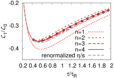
Fig. 1: (Color online) Comparison of the $\mathcal{L}$-moment equations obtained from various truncation of Eqs. (3) (lines), with those of the numerical solution of the kinetic equation (2) (symbols).

In the very early stage of high-energy heavy-ion collisions, the evolution of QGP system is dominated by the longitudinal expansion along the beam-axis. Accordingly, the evolution of QGP can be well approximated by Bjorken boost invariance and one is allowed to write the phase space distribution function as $f({\bf p},\tau)$. Given the phase space distribution, we introduce the $\mathcal{L}$-moment [5, 6],

$$\mathcal{L}_{n}=\int\frac{d^{3}p}{(2\pi)^{3}p^{0}}p^{2}P_{2n}(p_{z}/p_{\perp})f({\bf p},\tau)\,,$$ (1)

where $P_{2n}(x)$ is Legendre polynomial of order $2n$. ${\mathcal{L}}$-moments are of the same dimension as the energy-momentum tensor $T^{\mu\nu}$, but contains more detailed information of the anisotropic structure of $f$. One may check that the two lowest order moments, $\mathcal{L}_{0}$ and $\mathcal{L}_{1}$, coincide with energy density and pressure anisotropy, respectively. A vanishing $\mathcal{L}_{1}$ corresponds to isotropization. To derive the equations of motion for $\mathcal{L}_{n}$, for simplicity, we consider a transport equation with relaxation time approximation for the boost-invariant QGP,

$$\left[\partial_{\tau}-\frac{p_{z}}{\tau}\partial_{p_{z}}\right]f({\bf p},\tau)=-\frac{f({\bf p},\tau)-f_{\rm eq}(p/T)}{\tau_{R}},\qquad\tau_{R}=\tau_{R}(T)$$ (2)

where the relaxation time $\tau_{R}$ is a function of local temperature. Especially, throughout this paper, we consider a conformal system, $\tau_{R}\propto\eta/sT$. As will become clear later, the dimensionless quantity $\tau/\tau_{R}$ characterizes inverse of Knudsen number of the expanding system.

Eq. (2) leads a set of coupled equations for $\mathcal{L}_{n}$,

$$\frac{\partial\mathcal{L}_{n}}{\partial\tau}=-\frac{1}{\tau}\left[a_{n}\mathcal{L}_{n}+b_{n}\mathcal{L}_{n-1}+c_{n}\mathcal{L}_{n+1}\right]-\frac{\mathcal{L}_{n}}{\tau_{R}}(1-\delta_{n0}),\quad n=0,1,...$$ (3)

with $a_{n}$, $b_{n}$ and $c_{n}$ constant coefficients from the recursion relations of Legendre polynomials. One has to truncate Eq. (3) for practical analyses. A straightforward way to truncate Eq. (3) at order $n$ is to ignore all $\mathcal{L}$-moments higher than the n-th one. Especially, we notice that truncation at $n=0$ gives ideal hydro equation of motion. A test of the truncation is shown in Fig. 1. With respect to the evolution of $\mathcal{L}_{1}/\mathcal{L}_{0}$, from the case of truncation at $n=1$ to the case of truncation at $n=4$, one indeed observes a trend of convergence towards the exact solution (open symbols).

3 Fixed points of $\mathcal{L}$-moment equations and hydro attractors

There exist fixed-point solutions of Eq. (3) in two extreme cases. These fixed points are analyzed in terms of the following dimensionless quantity,

$$g_{n}=\tau\partial_{\tau}\ln\mathcal{L}_{n}\,,$$ (4)

which characterizes the decay rate of $\mathcal{L}$-moment regarding the system expansion. The first extreme with $\tau/\tau_{R}\rightarrow 0$ corresponds to the free-streaming evolution. In the free-streaming case, which amounts to very early time or sufficiently long relaxation time (or small coupling) in the expanding QGP system, one finds two fixed points: $g_{n}\approx-2$ and $g_{n}\approx-1$. Several comments are in order. First, it is not difficult to verify that only the one around $-1$ is a stable fixed point, which reflects the one-dimensional expansion of the system. Secondly, fixed points of all orders of $\mathcal{L}$-moments degenerate: $g_{0}=g_{1}=\ldots$. Lastly, the fixed points are found exact at $-2$ and $-1$ without truncation of the coupled $\mathcal{L}$-moment equations. However, truncation at any finite order will vary the expected value of fixed points. For intance, instead of -1, the stable fixed points are $g_{0}=g_{1}=-0.92937$ when truncating at $n=1$.

The opposite extreme $\tau/\tau_{R}\rightarrow\infty$ corresponds to the hydro limit, in which the system evolution reduces to hydrodynamics. To evaluate $g_{n}$ in this limit, we notice that the coupled equations of the $\mathcal{L}$-moments can be identified with hydro equation of motion. For truncation $n=0$, it trivially leads to the ideal hydro equation of motion. For the truncation at $n=1$, the coupled equations for $\mathcal{L}_{0}$ and $\mathcal{L}_{1}$ lead to the second order viscous hydro (Israel-Stewart),

$$\partial_{\tau}\mathcal{L}_{0}=-\frac{1}{\tau}(a_{0}\mathcal{L}_{0}+c_{1}\mathcal{L}_{1})\quad\rightarrow\quad\partial_{\tau}{\mathcal{E}}+\frac{{\mathcal{E}}+{\mathcal{P}}_{L}}{\tau}=0$$ (5)

$$\partial_{\tau}\mathcal{L}_{1}=-\frac{1}{\tau}(a_{1}\mathcal{L}_{1}+b_{1}\mathcal{L}_{0})-\frac{1}{\tau_{R}}\mathcal{L}_{1}\quad\rightarrow\quad\Pi=-\eta\sigma-a_{1}\frac{\tau_{R}}{\tau}\Pi-\tau_{R}\partial_{\tau}\Pi\,.$$ (6)

as long as one identifies $c_{0}\mathcal{L}_{1}=\Pi=\Pi^{\xi}_{\;\xi}$ as the $\xi$-$\xi$ component of the shear stress tensor. In Eq. (5), $\sigma=\sigma^{\xi}_{\;\xi}$ is the $\xi$-$\xi$ component of the tensor $\sigma^{\mu\nu}=2\langle\nabla^{\mu}u^{\nu}\rangle$. Similar strategy can generalized to truncation at arbitrary orders, and one recovers hydro equation of motion of higher orders. In these derivations, we notice that the leading order term in the gradient expansion of $\mathcal{L}_{n}$ is $\mathcal{L}_{n}\sim 1/\tau^{n}$, from which we find in the hydro limit, $g_{n}=-\frac{4+2n}{3}$. Note that these are stable fixed points depending on order $n$.

If initially starting from the stable free-streaming fixed point ($g_{n}\approx-1$), the system will evolve and finally approach to the hydro fixed points. These are special solutions of the system evolution, since any variation of these solutions will damp quickly due to the properties of fixed points, hence they are hydro attractors. Hydro attractor has been studied recently in various aspects, with respect to hydrodynamics [7], kinetic theory [8], and systems beyond Bjorken symmetry [9]. Numerically we have confirmed that hydro attractors identified between fixed points are consistent with what was found by other methods [8]. It should be emphasized that, in addition to the lowest order moment, $g_{0}\sim({\mathcal{P}}_{L}-{\mathcal{P}}_{T})/\epsilon$, there are infinite number of attractors in the evolving system.

4 Hydro attractors and renormalization of $\eta/s$

Fig. 2: Renormalization constant $Z_{\eta/s}$ as a function of $\tau/\tau_{R}$.

Considering the fact that attractor solutions extend the description of system evolution to out of equilibrium, we apply our hydro attractors to the formulation of out-of-equilibrium hydrodynamics. We understand that truncation at $n=2$ gives third order viscous hydrodynamics. To retain effects related to third or higher order viscous corrections, we rewrite the coupled equations as

$$\partial_{\tau}\mathcal{L}_{0}= -\frac{1}{\tau}(a_{0}\mathcal{L}_{0}+c_{0}\mathcal{L}_{1})\,,$$ (7)

$$\partial_{\tau}\mathcal{L}_{1}= -\frac{1}{\tau}(a_{1}\mathcal{L}_{1}+b_{0}\mathcal{L}_{0})-\left[1+\frac{c_{1}\tau_{R}}{\tau}\frac{\mathcal{L}_{2}}{\mathcal{L}_{1}}\right]\frac{\mathcal{L}_{1}}{\tau_{R}}$$ (8)

where the factor in the brackets (we define as $Z_{\eta/s}^{-1}$) is related to $g_{2}(\tau/\tau_{R})=-a_{2}-b_{2}\frac{\mathcal{L}_{2}}{\mathcal{L}_{1}}-\frac{\tau}{\tau_{R}}$. If one takes the attractor solution for $g_{2}$, higher order viscous effects are absorbed into $g_{2}$ through gradient summation. Accordingly, in Eq. (7), the factor $Z_{\eta/s}^{-1}$ effectively renormalizes the relaxation time $\tau_{R}$, or $\eta/s$. Fig. 2 presents the factor $Z_{\eta/s}^{-1}$ based on numerical solution of the hydro attractor, with respect to truncation at $n=3$ (leading order) and $n=4$ (next leading order). One notices that for system close to equilibrium ($\tau/\tau_{R}\rightarrow\infty$) the off-equilibrium effects are small, as expected. On the other hand, when the system is far away from equilibrium ($\tau/\tau_{R}\rightarrow 0$), the effective value of $\eta/s$ is largely reduced. The effect of $\eta/s$ renomralization can be further examined in practical simulations. A preliminary result is shown in Fig. 1 as the grey dashed line, which is solved numerically from the second order hydrodynamic equation but with a renormalized $\eta/s$. Comparing to the solution from second order hydro (truncation at $n=1$ in Fig. 1), improvement is remarkable.

5 Summary

We have proposed a set of $\mathcal{L}$-moments, whose equations of motion can be applied to describe out-of-equilibrium system evolution. These equations coincide with hydro equations of motion in the hydro regime. Hydro attractors can be found with respect to the $\mathcal{L}$-moments, and an effective renormalization of $\eta/s$ can be derived, which contains effects of out-of-equilibrium dynamics.

References

- [1] P. Kovtun, D. T. Son, A. O. Starinets, Viscosity in strongly interacting quantum field theories from black hole physics, Phys. Rev. Lett. 94 (2005) 111601. arXiv:hep-th/0405231, doi:10.1103/PhysRevLett.94.111601.
- [2] U. Heinz, R. Snellings, Collective flow and viscosity in relativistic heavy-ion collisions, Ann. Rev. Nucl. Part. Sci. 63 (2013) 123–151. arXiv:1301.2826, doi:10.1146/annurev-nucl-102212-170540.
- [3] G. Giacalone, L. Yan, J. Noronha-Hostler, J.-Y. Ollitrault, Skewness of elliptic flow fluctuations, Phys. Rev. C95 (1) (2017) 014913. arXiv:1608.01823, doi:10.1103/PhysRevC.95.014913.
- [4] V. Khachatryan, et al., Evidence for Collective Multiparticle Correlations in p-Pb Collisions, Phys. Rev. Lett. 115 (1) (2015) 012301. arXiv:1502.05382, doi:10.1103/PhysRevLett.115.012301.
- [5] J.-P. Blaizot, L. Yan, Onset of hydrodynamics for a quark-gluon plasma from the evolution of moments of distribution functions, JHEP 11 (2017) 161. arXiv:1703.10694, doi:10.1007/JHEP11(2017)161.
- [6] J.-P. Blaizot, L. Yan, Fluid dynamics of out of equilibrium boost invariant plasmas, Phys. Lett. B780 (2018) 283–286. arXiv:1712.03856, doi:10.1016/j.physletb.2018.02.058.
- [7] M. P. Heller, M. Spalinski, Hydrodynamics Beyond the Gradient Expansion: Resurgence and Resummation, Phys. Rev. Lett. 115 (7) (2015) 072501. arXiv:1503.07514, doi:10.1103/PhysRevLett.115.072501.
- [8] P. Romatschke, Relativistic Fluid Dynamics Far From Local Equilibrium, Phys. Rev. Lett. 120 (1) (2018) 012301. arXiv:1704.08699, doi:10.1103/PhysRevLett.120.012301.
- [9] G. S. Denicol, J. Noronha, Hydrodynamic attractor and the fate of perturbative expansions in Gubser flowarXiv:1804.04771.