Safe Reinforcement Learning via Probabilistic Shields

Abstract

This paper targets the efficient construction of a safety shield for decision making in scenarios that incorporate uncertainty. Markov decision processes (MDPs) are prominent models to capture such planning problems. Reinforcement learning (RL) is a machine learning technique to determine near-optimal policies in MDPs that may be unknown prior to exploring the model. However, during exploration, RL is prone to induce behavior that is undesirable or not allowed in safety- or mission-critical contexts. We introduce the concept of a probabilistic shield that enables decision-making to adhere to safety constraints with high probability. In a separation of concerns, we employ formal verification to efficiently compute the probabilities of critical decisions within a safety-relevant fragment of the MDP. We use these results to realize a shield that is applied to an RL algorithm which then optimizes the actual performance objective. We discuss tradeoffs between sufficient progress in exploration of the environment and ensuring safety. In our experiments, we demonstrate on the arcade game PAC-MAN and on a case study involving service robots that the learning efficiency increases as the learning needs orders of magnitude fewer episodes.

Introduction

Recent years showed increased use of reinforcement learning (RL) in solving tasks such as complex games (?) or robotic manipulation (?). In RL, an agent perceives the surrounding environment and acts towards maximizing a long-term reward signal. A major open challenge is the safety of decision-making for systems employing RL (?; ?). Particularly during the exploration phase, when an agent chooses random actions in order to examine its surroundings, it is important to avoid actions that may cause unsafe outcomes. The area of safe exploration investigates how RL agents can adhere to safety requirements during this phase (?; ?).

One suitable technique that delivers theoretical guarantees are so-called safety-shields (?; ?). Shields prevent an agent from taking unsafe actions at runtime. To this end, the performance objective is extended with a constraint specifying that unsafe states should never be visited. This new safety objective ensures there are no violations during the exploration phase. So far, shields have showed success in deterministic settings, where an agent avoids safety violations altogether. However, in many cases this tight restriction limits the agent’s exploration and understanding of the environment, and policies satisfying the restrictions may not even exist.

We propose to incorporate more liberal constraints that enforce safety violations to occur only with small probability. If an action increases the probability of a safety violation by more than a threshold $\delta$ with respect to the optimal safety probability, the shield blocks the action from the agent.

Consequently, an agent augmented with a shield is guided to satisfy the safety objective during exploration (or as long as the shield is used). The shield is adaptive with respect to $\delta$, as a high value for $\delta$ yields a stricter shield, a smaller value a more permissive shield. The value for $\delta$ can be changed on-the-fly, and may depend on the individual minimal safety probabilities at each state. Moreover, in case there is not suitable safe action with respect to $\delta$, the shield can always pick the optimal action as a fallback.

We base our formal notion of a probabilistic shield on MDPs, which constitute a popular modeling formalism for decision-making under uncertainty (?) and is widely used in model-based RL. We assess safety by means of probabilistic temporal logic constraints (?) that limit, for example, the probability to reach a set of critical states in the MDP.

In order to assess the risk of one action, we (1) construct a behavior model for the environment using model-based RL (?). We can plug this model into any concrete scenario to obtain an MDP. To construct the shield, we (2) use a model-based verification technique known as model checking (?; ?) that assesses whether a system model satisfies a specification. Due to its rigor, the validity of results only depends on the quality of the model, and we obtain precise safety probabilities of any possible decision within the MDP. These probabilities can be looked up efficiently and compared to the threshold $\delta$. The shield then readily (3) augments either model-free or model-based RL.

We identify three key challenges:

Firstly, model checking – as any model-based technique – is susceptible to scalability issues. A key advantage of using a separate safety objective is that we may analyze safety on just a fraction of the system, the safety-critical MDP. In our experiments, these MDP fragments are at least ten orders of magnitude smaller than a full model of the system, rendering model checking applicable to realistic scenarios. We introduce further optimizations based on problem-specific abstraction techniques.

Secondly, without randomness, all states are either absolutely safe or unsafe. However, in the presence of randomness, safety may be seen as a quantitative measure: in some states all actions may induce a large risk, while one action may be considered relatively safe. Therefore, it is essential to have an adaptive notion of shielding, in which the pre-selection of actions is not based on absolute thresholds.

Lastly, shielding may restrict exploration and lead to suboptimal policies. Therefore, it should not be considered in isolation. The trade-off between optimizing the performance objective and the achieved safety is intricate. Intuitively, accepting small short term risks may allow for efficient exploration and limit the risk long-term. To this end, we provide and discuss mechanisms that allow to adjust the shield based on such observations.

We apply shielding to two distinct use cases: the arcade game PACM-MAN and a new case study involving service robots in a warehouse. Shielded RL leads to improved policies for both case studies with fewer safety violations and performance superior to unshielded RL.

Supplementary materials are available at http://shieldrl.nilsjansen.org.

Related Work.

Most approaches to safe RL (?; ?) rely on reward engineering and effectively changing the learning objective. In contrast to ensuring temporal logic constraints, reward engineering designs or “tweaks” the reward functions such that a learning agent behaves in a desired, potentially safe, manner. As rewards are specialized for particular environments, reward engineering runs the risk of triggering negative side effects or hiding potential bugs (?). Recently, it was shown that reward engineering is not sufficient to capture temporal logic constraints in general (?). Additionally, in (?) the exploration of model-free RL algorithms is limited using control barrier functions and in (?) exploration is restricted to a space close to an optimal, precomputed policy.

First approaches directly incorporating formal specifications tackle this problem with pre-computations; making assumptions on the available information about the environment (?; ?; ?; ?; ?; ?), by employing PAC guarantees (?), or by an intermediate “correction” of policies (?). Most related is (?), which introduces the concept of a shield for RL. The difference and novel contribution is rooted in the consideration of stochastic behavior, which is natural to RL. Intuitively, without stochasticities, a learning agent does not take any risk, which is unrealistic in most scenarios. Moreover, often one cannot assume that a $100\%$ (or almost-sure) safety is realizable. A similar approach to ours was developed independently in (?), but targets a different case study and does not consider scalability issues of formal verification. In a related direction, methods from reinforcement learning have been successfully employed to improve the scalability of verification methods for MDPs. Such approaches often use rich specifications like $\omega$-regular languages as a control to guide the exploration of MDP during learning (?; ?; ?; ?; ?).

Safe model-based RL for continuous state spaces employing Lyapunov functions is considered in (?; ?). UPPAAL STRATEGO provides a number of algorithms combining safety synthesis with optimizing RL for continuous space MDPs (?). Finally, (?) uses control barrier functions (CBFs) for safe RL.

Probabilistic planning considers similar problems as probabilistic model checking (?; ?). A recent comparison between tools from both areas can be found in (?).

Problem Statement

Foundations.

A probability distribution over a countable set $X$ is a function $\mu\colon X\rightarrow[0,1]$ with $\sum_{x\in X}\mu(x)=1$. $\mathit{Distr}(X)$ denotes all distributions on $X$. The support of $\mu\in\mathit{Distr}(X)$ is $\mathit{supp}(\mu)=\{x\in X\mid\mu(x){>}0\}$. A Markov decision process (MDP) $\mathcal{M}{}=(S{},\mathit{Act}{},\mathcal{P}{},{r}{})$ has a set $S$ of states, a finite set $\mathit{Act}$ of actions, a (partial) probabilistic transition function $\mathcal{P}\colon S\times\mathit{Act}\rightarrow\mathit{Distr}(S)$, and an immediate reward function ${r}\colon S\times\mathit{Act}\rightarrow\mathbb{R}_{\geq 0}$. For all $s\in S$ the available actions are $\mathit{Act}(s)=\{\alpha\in\mathit{Act}\mid\mathcal{P}(s,\alpha)\neq\bot\}$ and we assume $|\mathit{Act}(s)|\geq 1$. A policy is a function $\sigma\colon S^{*}\rightarrow\mathit{Distr}(\mathit{Act})$ with $\mathit{supp}(\sigma(s_{1}\ldots s_{n}))\subseteq\mathit{Act}(s_{n})$ and $S^{*}$ a finite sequence of states.

In formal methods, safety properties are often specified as linear temporal logic (LTL) properties (?). For an MDP $\mathcal{M}$, probabilistic model checking (?; ?) employs value iteration or linear programming to compute the probabilities of all states and actions of the MDP to satisfy an LTL property $\varphi$. Specifically, we compute $\eta^{\max}_{\varphi,\mathcal{M}}\colon S\rightarrow[0,1]$ or $\eta^{\min}_{\varphi,\mathcal{M}}\colon S\rightarrow[0,1]$, which give for all states the minimal (or maximal) probability over all possible policies to satisfy $\varphi$. For instance, for $\varphi$ encoding to reach a set of states $T$, $\eta^{\max}_{\varphi,\mathcal{M}}(s)$ describes the maximal probability to “eventually” reach a state in $T$.

Setting.

We define a setting where one controllable agent (the avatar) and a number of uncontrollable agents (the adversaries) operate within an arena. The arena is a compact, high-level description of the underlying model. From this arena, the potential states and actions of all agents may be inferred. For safety considerations, the reward structure can be neglected, effectively reducing the state space for our model-based safety computations. Formally, an arena is a directed graph $G=(V,E)$ with a finite sets $V$ of nodes and $E\subseteq V\times V$ of edges. The agent’s position is defined via the current node $v\in V$. The agent decides on a new edge $(v,v^{\prime})\in E$ and determines its next position $v^{\prime}$.

Some (combinations of) agent positions are safety-critical, as they e.g. correspond to collisions or falling off a cliff. A safety property may describe reaching such positions, or use any other property expressible in (the safety fragment of) temporal logic.

While the underlying model for the arena suffices to specify the safe behavior, it is not sufficiently succinct to model the performance via rewards. Consider an edge that is safety-relevant, but the agent is only rewarded the first time taking this edge. Thus, in a flat model with rewards, two different edges are necessary to model this behavior. However, the reward (and thus the difference between these edges) is not needed to assess the safety, and the safety-relevant model may be pruned to an exponentially smaller model. We use a token function that implicitly extends the underlying model by a reward structure, enabling a separation of concerns between safety and performance.

Technically, we associate edges with a token function $\circ\colon E\rightarrow\{0,1\}$, indicating the status of an edge. Tokens can be (de-) activated and have an associated reward earned upon taking edges with an active token.

Example 1: Autonomous driving. An autonomous taxi (the avatar) operates within a road network encoded by an arena. The taxi has to visit several points to pick up or drop off passengers (?; ?). Upon visiting such a point, a corresponding token activates and a reward is earned, afterwards the token is deactivated permanently. Meanwhile, the taxi has to account for other traffic participants or further environmental factors (the adversaries). A sensible safety specification may restrict the probability for collision with other cars to $0.5\%$. Note that the token structure is not relevant for such a specification.

Example 2: Robot logistics in a smart factory. Take a factory floor plan with several corridors with machines. The adversaries are (possibly autonomous) transporters moving parts within the factory. The avatar models a specific service unit moving around and inspecting machines where an issue has been raised (as indicated by a token), while accounting for the behavior of the adversaries. Corridors might be to narrow for multiple (facing) robots, which poses a safety critical situation. The tokens allow to have a state-dependent cost, either as long as they are present (indicating the costs of a broken machine) or for removing the tokens (indicating costs for inspecting the machine). A similar scenario has been investigated in (?).

Problem.

Consider an environment described by an arena as above and a safety specification. We assume stochastic behaviors for the adversaries, e.g, obtained using RL (?; ?) in a training environment. In fact, this stochastic behavior determines all actions of the adversaries via probabilities. The underlying model is then a Markov decision process: the avatar executes an action, and upon this execution the next exact positions (the state of the system) are determined stochastically.

We compute a $\delta$-shield that prevents avatar decisions that violate this specification by more than a threshold $\delta$ with respect to the optimal safety probability. We evaluate the shield using a model-based or model-free RL avatar that aims to optimize the performance. The shield therefore has to handle an intricate tradeoff between strictly focussing on (short and midterm) safety and performance.

Constructing Shields for MDPs

Figure 1: Workflow of the Shield Construction

We outline the workflow of our approach in Fig. 1 and below. We employ a separation of concerns between the model-based shield construction and potentially model-free reinforcement learning (RL). First, we construct a behavior model for each adversary. Based on this model and a concrete arena, we construct a compact MDP model: the safety-relevant MDP quotient. In this MDP, we compute the shield which enables safe RL for the full MDP. We now detail the individual technical steps to realize our proposed method.

Behavior Models for Adversaries.

We learn an adversary model by observing behavior in a set of similar (small) arenas, until we gain sufficient confidence that more training data would not change the behavior significantly (?). An upper bound on the necessary data may be obtained using Hoeffding’s inequality (?). To reduce the size of the training set, we devise a data augmentation technique using domain knowledge of the arenas (?; ?). In particular, we abstract away from the precise configuration of the arena by partitioning the graph into zones that are relative to the view-point of the adversary (e. g., near or far, north or south, east or west). The intuitive assumption is that the specific position of an adversary is not important, but some key information is (e.g., the relation to the position of the avatar). This approach (1) speeds up the learning process and (2) renders the resulting behavior model applicable for varying the concrete instance of the same setting.

Zones are uniquely identified by a coloring with a finite set $C$ of colors. Formally, for an arena $G=(V,E)$, zones relative to a node $v\in V$ are given by a function $z_{v}\colon V\rightarrow C$. For nodes $x,y\in V$, with $z_{v}(x)=z_{v}(y)$, the assumption is that the adversary in $v$ behaves similarly regardless whether the avatar is in $x$ or $y$. From our observations, we extract a histogram $h\colon E\times C\rightarrow\mathbb{N}$, where $h(e,c)$ describes how often the adversary takes an edge $e=(v,v^{\prime})\in E$ while the avatar is in a node $u$ with $z_{v}(u)=c$. We translate these likelihoods into distributions over possible edges in the arena.

Definition 1 (Adversary Behavior).

For an arena $G=(V,E)$, zones $z_{u}\colon V\rightarrow C$ for every $u\in V$, and a histogram $h\colon E\times C\rightarrow\mathbb{N}$, the adversary behavior is a function $B\colon V\times C\rightarrow\mathit{Distr}(E)$ with

$$B(v,c)=\frac{h\big{(}(v,v^{\prime}),c\big{)}}{\sum_{(v,v^{\prime})\in E}h\big{(}(v,v^{\prime}),c\big{)}}\ .$$

While we employ a simple normalization of likelihoods, alternatively one may also utilize, e. g., a softmax function which is adjustable to favor more or less likely decisions (?).

Safety-Relevant Quotient MDP.

The construction of the MDP $\mathcal{M}{}=(S{},\mathit{Act}{},\mathcal{P}{})$ augments an arena by behavior models $B_{i}$. First, the states $S=V^{m+1}\times\{0,\ldots,m\}$ encode the positions for all agents and whose turn it is. The decision states of the safety-relevant MDP $\mathcal{M}$ are $S_{d}=\{s_{d}\in S\mid s_{d}=(\ldots,0)\}$, i.e., it’s the turn of the avatar. The actions $\mathit{Act}=\{\alpha_{0}\}\cup\mathit{Act}_{E}$ with $\mathit{Act}_{E}=\{\alpha_{e}\mid e\in E\}$ determine the movements of the avatar and the adversaries. For $(v,\ldots,0)=s_{d}\in S_{d}$ (the avatar moves next), the available actions are $\alpha_{e}\in\mathit{Act}(s_{d})\subseteq\mathit{Act}_{e}$, where $\alpha_{e}$ corresponds to an outgoing edge of $v$. For $(v,\ldots,0)=s_{d}\in S_{d}$, $\alpha_{e}$ with $e=(v,v^{\prime})$ leads with probability one to a state $s_{e}=(v^{\prime},\ldots,1)$. For $(v,\ldots,v_{i},\ldots,i>0)$ (an adversary moves next), there is a unique action $\alpha_{0}$ where $v_{i}$ is changed to $v^{\prime}_{i}$, randomly determined according to the behavior $B_{i}$, which also updates $i$ to $i+1$ modulo $m$. These transitions induce the only probabilistic choices in the MDP.

A policy only has to choose an action at decision states. At all other states, only the unique action $\alpha_{0}$ emanates. Consequently, a policy for $\mathcal{M}$ is a policy for the avatar.

In theory, one can build the full MDP for the arena $(V,E)$ and the token function $\circ\colon E\rightarrow\{0,1\}$ under the assumption that the reward function is known. Then, one can compute the reward-optimal and safe policy without need for further learning techniques. As there are $2^{E}$ token configurations, the state space blows up exponentially, which prevents the successful application of model checking or planning techniques for anything but very small applications.

Shield Construction.

For the safety-relevant MDP $\mathcal{M}$, a set of unsafe states $T\subseteq S$ should preferably not be reached from any state. The property $\varphi=\lozenge T$ encodes the violation of this safety constraint, that is, eventually reaching $T$ within $\mathcal{M}$. The shield needs to limit the probability to satisfy $\varphi$. We evaluate all decision states $s_{d}\in S_{d}$ with respect to this probability: We compute $\eta^{\min}_{\varphi,\mathcal{M}}(s_{e})$, i.e., the minimal probability to satisfy $\varphi$ from $s_{e}$, which is the state reached after taking action $\alpha_{e}\in\mathit{Act}_{e}$ in $s_{d}$.

Definition 2 (Action-valuation).

An action-valuation for action $\alpha_{e}\in\mathit{Act}_{e}$ at state $s_{d}\in S_{d}$ is

$$\textsl{val}_{s_{d}}^{\mathcal{M}}\colon\mathit{Act}(s_{d})\rightarrow[0,1]\text{, with }\textsl{val}_{s_{d}}^{\mathcal{M}}(\alpha_{e})=\eta^{\min}_{\varphi,\mathcal{M}}(s_{e})\ .$$

The optimal action-value for $s_{d}$ is $\textsl{optval}_{s_{d}}^{\mathcal{M}}=\min_{\alpha^{\prime}\in\mathit{Act}}\textsl{val}_{s_{d}}^{\mathcal{M}}(\alpha^{\prime})$, the set of all action-valuations at $s_{d}$ is $\textsl{ActVals}_{s_{d}}$.

We now define a shield for the safety-relevant MDP $\mathcal{M}$ using the action values. Specifically, a $\delta$-shield for $\delta\in[0,1]$ determines a set of actions at each decision state $s_{d}$ that are $\delta$-optimal for the specification $\varphi$. All other actions are “shielded” or “blocked”.

Definition 3 (Shield).

For action-valuation $\textsl{val}_{s_{d}}^{\mathcal{M}}$ and $\delta\in[0,1]$, a $\delta$-shield for state $s_{d}\in S_{d}$ is

$$\textsl{shield\,}_{\delta}^{s_{d}}\colon \textsl{ActVals}_{s_{d}}\rightarrow 2^{\mathit{Act}(s_{d})}$$

with $\textsl{shield\,}_{\delta}^{s_{d}}\mapsto\{\alpha\in\mathit{Act}(s_{d})\mid\delta\cdot\textsl{val}_{s_{d}}^{\mathcal{M}}(\alpha)\leq\textsl{optval}_{s_{d}}^{\mathcal{M}}\}.$

Intuitively, $\delta$ enforces a constraint on actions that are acceptable with respect to the optimal probability. The shield is adaptive with respect to $\delta$, as a high value for $\delta$ yields a stricter shield, a smaller value a more permissive shield. The shield is stored using a lookup-table, and the value for $\delta$ can then be changed on-the-fly. In particularly critical situations, the shield can enforce the decision-maker to resort to (only) the optimal actions w.r.t. the safety objective.

A $\delta$-shield for the MDP $\mathcal{M}$ is built by constructing and applying $\delta$-shields to all decision states.

Definition 4 (Shielded MDP).

The shielded MDP $\mathcal{M}_{\text{\raisebox{-1.5pt}{ \leavevmode\hbox to4.92pt{\vbox to5.67pt{\text{[drawing]}}}}}}=(S,\mathit{Act}\,\mathcal{P}_{\text{\raisebox{-1.5pt}{ \leavevmode\hbox to4.92pt{\vbox to5.67pt{\text{[drawing]}}}}}})$ for a safety-relevant quotient MDP $\mathcal{M}{}=(S{},\mathit{Act}{},\mathcal{P}{})$ and a $\delta$-shield for all $s_{d}\in S_{d}$ is given by the transition probability $\mathcal{P}_{\text{\raisebox{-1.5pt}{ \leavevmode\hbox to4.92pt{\vbox to5.67pt{\text{[drawing]}}}}}}$ with $\mathcal{P}_{\text{\raisebox{-1.5pt}{ \leavevmode\hbox to4.92pt{\vbox to5.67pt{\text{[drawing]}}}}}}(s,\alpha)=\mathcal{P}(s,\alpha)$ if $\alpha\in\textsl{shield\,}_{\delta}^{s}(\textsl{val}_{s}^{\mathcal{M}})$ and $\mathcal{P}_{\text{\raisebox{-1.5pt}{ \leavevmode\hbox to4.92pt{\vbox to5.67pt{\text{[drawing]}}}}}}(s,\alpha)=\bot$ otherwise.

Lemma 1.

If MDP $\mathcal{M}$ is deadlock-free if and only if the shielded MDP $\mathcal{M}_{\text{\raisebox{-1.5pt}{ \leavevmode\hbox to4.92pt{\vbox to5.67pt{\text{[drawing]}}}}}}$ is deadlock-free.

We compute the shield relative to optimal values $\textsl{optval}_{s_{d}}^{\mathcal{M}}$. Consequently, for $\delta=1$, only optimal actions are preserved, and for $\delta=0$ no actions are blocked.

Theorem 1.

For an MDP $\mathcal{M}$ and a $\delta$-shield, it holds for any state $s$ that $\textsl{val}_{s}^{\mathcal{M}}=\textsl{val}_{s}^{\mathcal{M}_{\text{\raisebox{-1.5pt}{ \leavevmode\hbox to3.63pt{\vbox to4.17pt{\text{[drawing]}}}}}}}$.

As optimal actions for the safety objective are not removed, optimality w.r.t. safety is preserved in the shielded MDP. Thus, during construction of the shield, we compute the action-valuations in fact for the shielded MDP. Observe that computing a shield for a state is done independently from the application of the shield to other states.

Guaranteed Safety.

A $\delta$-shield ensures that only actions that are $\delta$-optimal with respect to an LTL property $\varphi$ are allowed. In particular, for each action $\alpha\in\mathit{Act}_{e}$ at state $s_{e}$, we use the minimal probability $\eta^{\min}_{\varphi,\mathcal{M}}(s_{e})$ to satisfy $\varphi$, see Def. 2. Under optimal (subsequent) choices, the value $\eta^{\min}_{\varphi,\mathcal{M}}(s_{e})$ will be achieved. In contrast, a sequence of bad choices may violate $\varphi$ with high probability. A more conservative notion would be to use the minimal action value while assuming that in all subsequent states the worst-case decisions corresponding to the maximal probabilities are taken. These values are computable by model checking. Regardless of subsequent choices, at least $\textsl{val}_{s_{d}}^{\mathcal{M}}(\alpha_{e})$ is then guaranteed. A sensible notion to construct a shield would then be to impose a threshold $\lambda\in[0,1]$ such that only actions with $\textsl{val}_{s_{d}}^{\mathcal{M}}(\alpha_{e})\leq\lambda$ are allowed. A shield with such a guaranteed safety probability may induce a shielded MDP (Def. 4) that is not deadlock free. Moreover, the shield may become too restrictive for the agent.

Scalable Shield Construction.

Although we apply model checking only in the safety-relevant MDP, scalability issues for large applications remain. We employ several optimizations towards computational tractability.

Finite Horizon. For infinite horizon properties, the probability to violate safety (in the long run) is often one. Furthermore, our learned MDP model is inherently an approximation of the real world. Errors originating from this approximation accumulate for growing horizons. Thus, we focus on a finite horizon such that the action values (and consequently, a policy for the avatar) carry only guarantees for the next steps. This assumption also allows us to prune the safety-relevant MDP (see below), increasing the scalability.

Piecewise Construction. Computing a shield for all states in an MDP concurrently yields a large memory footprint. To alleviate this footprint, we compute the shield states independently, in accordance with Theorem 1. The independent computation prunes the relevant part of the MDP, as the number of states reachable within the horizon is drastically reduced. Additionally, the independent computation allows for parallelizing the computation.

Independent Agents. The explosion of state spaces stems mostly from the number of agents. Here, an important observation is that we can consider agents independently. For instance, the probability for the avatar to crash with an adversary is stochastically independent from crashing with the others. Instead of determining the shield for all adversaries at once, we perform computations for each agent individually, and combine them via the inclusion-exclusion principle. Afterwards, the shield is composed from the shields dedicated to individual adversaries.

Abstractions. We observe that for finite horizon properties and piecewise construction, adversaries may be far away—beyond the horizon—without a chance to reach the avatar. We do not need to consider such (positions for) adversaries, as in these states, the shield will not block any actions.

Fewer Decision States. Depending on the setting, there might be only a few critical situations in which the agent requires shielding to ensure safety. The shield can be computed for this critical states only. Consequently, the agent makes shielded decisions in the adapted decision states, and unshielded decisions in all other ones.

Shielding versus Performance.

A shield which is minimally invasive gives the RL agent the most freedom to optimize the performance objective. We propose two methods to alleviate invasiveness, all of them assume domain knowledge of the rationale behind the decision procedure.

Iterative Weakening. During runtime, we may observe that the progress of the avatar regarding the performance objective is not increasing anymore. Then, we weaken the shield by $\delta-\varepsilon$, allowing additional actions. As soon as progress is made, we reset $\delta$ to its former value. The adaption of $\textsl{shield\,}_{\delta}^{s}$ to $\textsl{shield\,}_{\delta-\varepsilon}^{s}$ can be done on the fly, without new computations.

Adapted Specifications. If the goal of the decision maker is known and can be captured in temporal logic, we may adapt the original specification accordingly. There are often natural trade-offs between safety and performance. These trade-offs might be resolved via weights, but this process is often undesirable (?) and similar to reward engineering. Instead, optimizing the conditional performance while assuming to stay sufficiently safe (?), avoids side-effects of attaching some weights to the safety specification.

Implementation and Numerical Experiments

Set-up.

We run experiments using an Intel Core i7-4790K CPU with 16 GB of RAM using 4 cores. We give the timing results for a single CPU. Since the shield may be computed in a multi-threaded architecture, this time can be divided by the number of cores available.

The supplementary materials, namely the source code and videos are available online.

We demonstrate the applicability of our approach by means of two case studies. For both case studies, we learn adversary behavior in small arenas individually for each adversary. These behavior models are applicable to any benchmark instance, as they are independent of concrete positions.

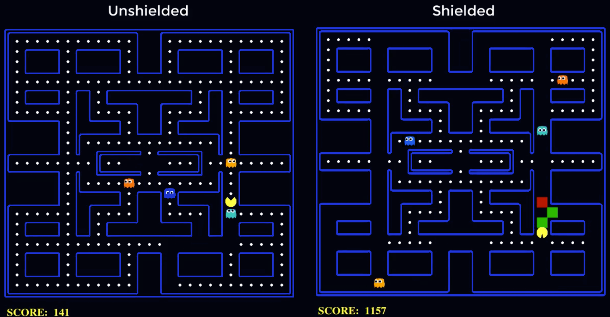
(a) Still from video on classic PAC-MAN

(b) Scores during training for classic PAC-MAN

Figure 2: Scenarios and results for PAC-MAN

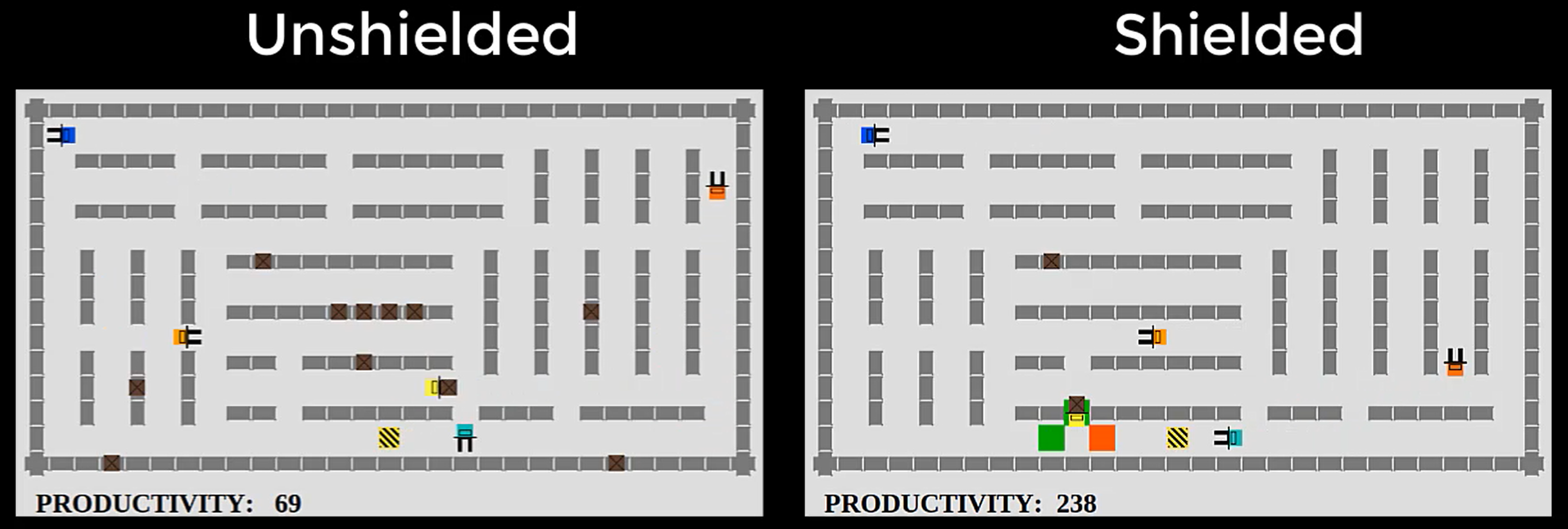
(a) Still from the video on warehouse

(b) Scores during training on warehouse

Figure 3: Scenarios and results for warehouse

For the arcade game PAC-MAN, PM (the avatar) aims to collect PAC-dots in a maze and not get caught by ghosts (the adversaries). We model various instance of the game (with different sizes) as an arena, where tokens represent the dots at each position in the maze, such that a dot is either present or collected. The score (reward, performance) is positively affected (+10) by collecting a dot and negatively by time (each step: -1). If PM either collects all dots (+500) or is caught (-500), the game is restarted. RL approaches exist (?), but they suffer from the fact that during the exploration phase PM is often caught by the ghosts, achieving very poor scores. The safety specification places a lower bound on the probability of reaching states in the underlying MDP that correspond to being caught.

We also consider a warehouse floor plan with several corridors. A similar scenario has been investigated in (?). In the arena, nodes describe crossings, the edges the corridors with shelves, and the distances the corridor length. The agents are fork-lift units picking up packages from the shelves and delivering them to the exit; tokens represent the presence of a package at its position. The avatar is a specific (yellow) fork-lift unit that has to account for other units, the adversaries. The performance (reward) is positively affected by loading and delivering packages (+20, respectively) and negatively by time (each step: -1). Delivering all packages yields a large bonus (+500) and a collision leads to a large punishment (-500), both cases end the scenario. Corridors might be too narrow for multiple (facing) units, which poses a safety-critical situation. Most crucial is the crowded area near the exit, since all units have to deliver the packages to the exit.

Transferring the stochastic adversary behavior to any arena (without tokens) yields a concrete safety-relevant MDP. In particular, we specify an arena with the positions of the avatar and the adversaries as well as the behavior in the high-level PRISM-language (?). We employ a script that automatically generates arenas to enable a broad set of benchmarks. Taking, e.g., the PAC-MAN arena from Fig. 2(a), the considered MDP has roughly $10^{12}$ states (compared to $10^{50}$ for the full MDP). For a safety-relevant MDP, we compute a $\delta$-shield (with iterative weakening) via the model checker Storm (?), using a horizon of $10$ steps. The immense size even of safety-relevant MDPs requires optimizations such as a piecewise and independent shield construction. Moreover, a multi-threaded architecture lets us construct shields for very large examples. In particular, we perform model checking for (many) MDPs of roughly $10^{6}$ states. The computation time for the largest PM instance takes about 6 hours (single-threaded), while memory is not an issue due to the piecewise shield construction.

We compare RL to shielded RL on different instances. The key comparison criterion is the performance (detailed above) during learning. Our implementation is based on an existing PAC-MAN environment using an approximate Q-learning agent (?) with the following feature vectors:

• for PAC-MAN: (1) distance to the closest dot, (2) whether a ghost collision is imminent, and (3) whether a ghost is one step away.

• for Warehouse: (1) has the unit loaded or unloaded, (2) the distance to the next package and (3) to the exit, (4) whether another unit is three steps away and (5) one step away.

The results are basic reflex controllers. The Q-learning uses the learning rate $\alpha=0.2$ and the discount factor $\gamma=0.8$ for the Q-update and an $\epsilon$-greedy exploration policy with $\epsilon=0.05$. One episode lasts until either the game is restarted. We describe results for the training phase of RL (300 episodes).

Results.

Figures 2(a) and 3(a) show screenshots of a series of recommended videos (available in the supplementary material). Each video compares how RL performs either shielded or unshielded on a instance of the case study. In the shielded version, at each decision state in the underlying MDP, we indicate the risk of decisions from low to high by the colors green, orange, red.

Consider PAC-MAN in detail: Figure 2(b) depicts the scores obtained during RL. The curves (blue, solid: unshielded, orange, dashed: shielded) show the average scores for every ten training episodes. Table 1 shows results for instances in increasing size. We list the number of model checking calls and the time to construct the shield. We list the scores with and without shield, and the winning rate capturing the ratio of successfully ended episodes. For all instances, we see a large difference in scores due to the fact that PM is often rescued by the shield. The winning rates differ for most benchmarks, favoring shielded RL. For three or four ghosts, a shield with a ten-step horizon cannot guide PM to avoid being encircled by the ghosts long enough to successfully end the game. Nevertheless, the shield often safes PM, leading to superior scores. Moreover, the shield helps learning an optimal policy much faster as fewer restarts are needed.

For the warehouse case study, we choose to vary the decision states, i.e., the positions of the avatar for which we compute a shield. We present results for shielding the 2–8 crossings closest to the exit. Figure 3(b) shows the average score for the different variants, Table 2 summarizes average score and win rate. Unsurprisingly, the score gets better the more states are shielded. Furthermore, we have seen that shielding even more states has only a very limited effect.

Table 1: Average scores and win rates for PM

Size, #Ghosts	#Model Checking	time (s)	Score w/o Shield	Score w. Shield	Win Rate w/o Shield	Win Rate w. Shield
9x7,1	5912	584	-359,6	535,3	0,04	0,84
17x6,2	5841	1072	-195,6	253,9	0,04	0,4
17x10,3	51732	3681	-220,79	-40,52	0,01	0,07
27x25,4	269426	19941	-129,25	339,89	0,00	0,00

Table 2: Average scores and win rates for warehouse

Crossings shielded	0	2	4	8
Score	-186	-27.6	303	420
Win Rate	0.16	0.31	0.59	0.71

Conclusion and Future Work

We developed the concept of shields for MDPs. Utilizing probabilistic model checking, we maintained probabilistic safety measures during reinforcement learning. We addressed inherent scalability issues and provided means to deal with typical trade-off between safety and performance. Our experiments showed that we improved the state-of-the-art in safe reinforcement learning.

For future work, we will extend shields to richer models such as partially-observable MDPs. Moreover, we will extend the applications to more arcade games and employ deep recurrent neural networks as means of decision-making (?; ?). Another interesting direction is to explore (possibly model-free) learning of shields, instead of employing model-based model checking.

References

- [Alshiekh et al. 2018] Alshiekh, M.; Bloem, R.; Ehlers, R.; Könighofer, B.; Niekum, S.; and Topcu, U. 2018. Safe reinforcement learning via shielding. In AAAI. AAAI Press.
- [Amodei et al. 2016] Amodei, D.; Olah, C.; Steinhardt, J.; Christiano, P.; Schulman, J.; and Mané, D. 2016. Concrete problems in AI safety. CoRR abs/1606.06565.
- [Baier and Katoen 2008] Baier, C., and Katoen, J. 2008. Principles of Model Checking. MIT Press.
- [Berkeley 2018] Berkeley, U. 2018. Intro to AI – Reinforcement Learning . http://ai.berkeley.edu/reinforcement.html.
- [Berkenkamp et al. 2017] Berkenkamp, F.; Turchetta, M.; Schoellig, A.; and Krause, A. 2017. Safe model-based reinforcement learning with stability guarantees. In NIPS, 908–919.
- [Bit-Monnot et al. 2018] Bit-Monnot, A.; Leofante, F.; Pulina, L.; Ábrahám, E.; and Tacchella, A. 2018. Smartplan: a task planner for smart factories. CoRR abs/1806.07135.
- [Bloem et al. 2015] Bloem, R.; Könighofer, B.; Könighofer, R.; and Wang, C. 2015. Shield synthesis: - runtime enforcement for reactive systems. In TACAS, volume 9035 of LNCS, 533–548. Springer.
- [Bouton et al. 2019] Bouton, M.; Karlsson, J.; Nakhaei, A.; Fujimura, K.; Kochenderfer, M. J.; and Tumova, J. 2019. Reinforcement learning with probabilistic guarantees for autonomous driving. CoRR abs/1904.07189.
- [Brázdil et al. 2014] Brázdil, T.; Chatterjee, K.; Chmelík, M.; Forejt, V.; Křetínský, J.; Kwiatkowska, M. Z.; Parker, D.; and Ujma, M. 2014. Verification of Markov decision processes using learning algorithms. In ATVA.
- [Carr et al. 2019] Carr, S.; Jansen, N.; Wimmer, R.; Serban, A. C.; Becker, B.; and Topcu, U. 2019. Counterexample-guided strategy improvement for pomdps using recurrent neural networks. In IJCAI, 5532–5539. ijcai.org.
- [Cheng et al. 2019] Cheng, R.; Orosz, G.; Murray, R. M.; and Burdick, J. W. 2019. End-to-end safe reinforcement learning through barrier functions for safety-critical continuous control tasks. AAAI.
- [Chow et al. 2018] Chow, Y.; Nachum, O.; Duenez-Guzman, E.; and Ghavamzadeh, M. 2018. A Lyapunov-based approach to safe reinforcement learning. In NIPS, 8103–8112.
- [Clarke, Grumberg, and Peled 2001] Clarke, E. M.; Grumberg, O.; and Peled, D. A. 2001. Model checking. MIT Press.
- [David et al. 2015] David, A.; Jensen, P. G.; Larsen, K. G.; Mikucionis, M.; and Taankvist, J. H. 2015. Uppaal stratego. In TACAS, volume 9035 of LNCS, 206–211. Springer.
- [Dayan and Niv 2008] Dayan, P., and Niv, Y. 2008. Reinforcement learning: the good, the bad and the ugly. Current opinion in neurobiology 18(2):185–196.
- [Dehnert et al. 2017] Dehnert, C.; Junges, S.; Katoen, J.; and Volk, M. 2017. A storm is coming: A modern probabilistic model checker. In CAV (2), volume 10427 of LNCS, 592–600. Springer.
- [Dietterich 2000] Dietterich, T. G. 2000. Hierarchical reinforcement learning with the maxq value function decomposition. Journal of Artificial Intelligence Research 13:227–303.
- [Freedman and Zilberstein 2016] Freedman, R. G., and Zilberstein, S. 2016. Safety in AI-HRI: Challenges complementing user experience quality. In AAAI Fall Symposium Series.
- [Fu and Topcu 2014] Fu, J., and Topcu, U. 2014. Probably approximately correct mdp learning and control with temporal logic constraints. In RSS.
- [Fulton and Platzer 2019] Fulton, N., and Platzer, A. 2019. Verifiably safe off-model reinforcement learning. 11427:413–430.
- [Garcıa and Fernández 2015] Garcıa, J., and Fernández, F. 2015. A comprehensive survey on safe reinforcement learning. Journal of Machine Learning Research 16(1):1437–1480.
- [García and Fernández 2019] García, J., and Fernández, F. 2019. Probabilistic policy reuse for safe reinforcement learning. ACM Transactions on Autonomous and Adaptive Systems (TAAS) 13(3):14.
- [Gym 2018] Gym, O. 2018. Taxi-v2. https://gym.openai.com/envs/Taxi-v2/.
- [Hahn et al. 2018] Hahn, E. M.; Perez, M.; Schewe, S.; Somenzi, F.; Trivedi, A.; and Wojtczak, D. 2018. Omega-regular objectives in model-free reinforcement learning. CoRR abs/1810.00950.
- [Hahn et al. 2019a] Hahn, E. M.; Hartmanns, A.; Hensel, C.; Klauck, M.; Klein, J.; Kretínský, J.; Parker, D.; Quatmann, T.; Ruijters, E.; and Steinmetz, M. 2019a. The 2019 comparison of tools for the analysis of quantitative formal models - (qcomp 2019 competition report). In TACAS (3), volume 11429 of LNCS, 69–92. Springer.
- [Hahn et al. 2019b] Hahn, E. M.; Perez, M.; Schewe, S.; Somenzi, F.; Trivedi, A.; and Wojtczak, D. 2019b. Omega-regular objectives in model-free reinforcement learning. In TACAS (1), volume 11427 of LNCS, 395–412. Springer.
- [Hasanbeig, Abate, and Kroening 2018] Hasanbeig, M.; Abate, A.; and Kroening, D. 2018. Logically-correct reinforcement learning. CoRR abs/1801.08099.
- [Hausknecht and Stone 2015] Hausknecht, M., and Stone, P. 2015. Deep recurrent q-learning for partially observable mdps. CoRR, abs/1507.06527.
- [Junges et al. 2016] Junges, S.; Nils Jansen; Dehnert, C.; Topcu, U.; and Katoen, J. 2016. Safety-constrained reinforcement learning for MDPs. In TACAS, volume 9636 of LNCS, 130–146. Springer.
- [Katoen 2016] Katoen, J.-P. 2016. The probabilistic model checking landscape. In LICS, 31–45. ACM.
- [Kolobov 2012] Kolobov, A. 2012. Planning with Markov decision processes: An AI perspective. Synthesis Lectures on Artificial Intelligence and Machine Learning 6(1):1–210.
- [Kretínský, Pérez, and Raskin 2018] Kretínský, J.; Pérez, G. A.; and Raskin, J. 2018. Learning-based mean-payoff optimization in an unknown MDP under omega-regular constraints. In CONCUR, volume 118 of LIPIcs, 8:1–8:18. Schloss Dagstuhl - Leibniz-Zentrum fuer Informatik.
- [Krizhevsky, Sutskever, and Hinton 2012] Krizhevsky, A.; Sutskever, I.; and Hinton, G. E. 2012. Imagenet classification with deep convolutional neural networks. In NIPS, 1097–1105.
- [Kwiatkowska, Norman, and Parker 2011] Kwiatkowska, M. Z.; Norman, G.; and Parker, D. 2011. PRISM 4.0: Verification of probabilistic real-time systems. In CAV, volume 6806 of LNCS, 585–591. Springer.
- [Kwiatkowska 2003] Kwiatkowska, M. Z. 2003. Model checking for probability and time: from theory to practice. In LICS, 351. IEEE CS.
- [Mason et al. 2017] Mason, G.; Calinescu, R.; Kudenko, D.; and Banks, A. 2017. Assured reinforcement learning with formally verified abstract policies. In ICAART (2), 105–117. SciTePress.
- [Moldovan and Abbeel 2012] Moldovan, T. M., and Abbeel, P. 2012. Safe exploration in markov decision processes. In ICML. icml.cc / Omnipress.
- [Ohnishi et al. 2019] Ohnishi, M.; Wang, L.; Notomista, G.; and Egerstedt, M. 2019. Barrier-certified adaptive reinforcement learning with applications to brushbot navigation. IEEE Transactions on Robotics 1–20.
- [Pathak et al. 2015] Pathak, S.; Ábrahám, E.; Jansen, N.; Tacchella, A.; and Katoen, J. 2015. A greedy approach for the efficient repair of stochastic models. In NFM, volume 9058 of LNCS, 295–309.
- [Pecka and Svoboda 2014] Pecka, M., and Svoboda, T. 2014. Safe exploration techniques for reinforcement learning–an overview. In MESAS, 357–375. Springer.
- [Pnueli 1977] Pnueli, A. 1977. The temporal logic of programs. In Foundations of Computer Science, 46–57. IEEE.
- [Roijers et al. 2013] Roijers, D. M.; Vamplew, P.; Whiteson, S.; and Dazeley, R. 2013. A survey of multi-objective sequential decision-making. J. Artif. Intell. Res. 48:67–113.
- [Sadigh et al. 2014] Sadigh, D.; Kim, E. S.; Coogan, S.; Sastry, S. S.; and Seshia, S. A. 2014. A learning based approach to control synthesis of markov decision processes for linear temporal logic specifications. In CDC, 1091–1096. IEEE.
- [Sadigh et al. 2016] Sadigh, D.; Sastry, S.; Seshia, S. A.; and Dragan, A. D. 2016. Planning for autonomous cars that leverage effects on human actions. In Robotics: Science and Systems.
- [Sadigh et al. 2018] Sadigh, D.; Landolfi, N.; Sastry, S. S.; Seshia, S. A.; and Dragan, A. D. 2018. Planning for cars that coordinate with people: leveraging effects on human actions for planning and active information gathering over human internal state. Autonomous Robots 42(7):1405–1426.
- [Sculley et al. 2014] Sculley, D.; Phillips, T.; Ebner, D.; Chaudhary, V.; and Young, M. 2014. Machine learning: The high-interest credit card of technical debt.
- [Silver et al. 2016] Silver, D.; Huang, A.; Maddison, C. J.; Guez, A.; Sifre, L.; Van Den Driessche, G.; Schrittwieser, J.; Antonoglou, I.; Panneershelvam, V.; Lanctot, M.; et al. 2016. Mastering the game of go with deep neural networks and tree search. nature 529(7587):484.
- [Steinmetz, Hoffmann, and Buffet 2016] Steinmetz, M.; Hoffmann, J.; and Buffet, O. 2016. Goal probability analysis in probabilistic planning: Exploring and enhancing the state of the art. J. Artif. Intell. Res. 57:229–271.
- [Stoica et al. 2017] Stoica, I.; Song, D.; Popa, R. A.; Patterson, D.; Mahoney, M. W.; Katz, R.; Joseph, A. D.; Jordan, M.; Hellerstein, J. M.; Gonzalez, J. E.; et al. 2017. A berkeley view of systems challenges for AI. CoRR abs/1712.05855.
- [Sutton and Barto 1998] Sutton, R. S., and Barto, A. G. 1998. Reinforcement Learning: An Introduction. MIT Press.
- [Teichteil-Königsbuch 2012] Teichteil-Königsbuch, F. 2012. Stochastic safest and shortest path problems. In AAAI. AAAI Press.
- [Wang et al. 2019] Wang, A.; Kurutach, T.; Liu, K.; Abbeel, P.; and Tamar, A. 2019. Learning robotic manipulation through visual planning and acting. arXiv preprint arXiv:1905.04411.
- [Wen, Ehlers, and Topcu 2015] Wen, M.; Ehlers, R.; and Topcu, U. 2015. Correct-by-synthesis reinforcement learning with temporal logic constraints. In IROS.
- [White 1985] White, D. J. 1985. Real applications of Markov decision processes. Interfaces 15(6):73–83.
- [Witten et al. 2016] Witten, I. H.; Frank, E.; Hall, M. A.; and Pal, C. J. 2016. Data Mining: Practical machine learning tools and techniques. Morgan Kaufmann.
- [Ziebart et al. 2008] Ziebart, B. D.; Maas, A. L.; Bagnell, J. A.; and Dey, A. K. 2008. Maximum entropy inverse reinforcement learning. In AAAI, 1433–1438. AAAI Press.