Evolution of galaxy size–stellar mass relation from the Kilo Degree Survey

Abstract

We have obtained structural parameters of about $340,000$ galaxies from the Kilo Degree Survey (KiDS) in 153 square degrees of data release 1, 2 and 3. We have performed a seeing convolved 2D single Sérsic fit to the galaxy images in the 4 photometric bands ($u$, $g$, $r$, $i$) observed by KiDS, by selecting high signal-to-noise ratio ($\mbox{$S/N$}>50$) systems in every bands.

We have classified galaxies as spheroids and disc-dominated by combining their spectral energy distribution properties and their Sérsic index. Using photometric redshifts derived from a machine learning technique, we have determined the evolution of the effective radius, $R_{\rm e}$ and stellar mass, $M_{\star}$, versus redshift, for both mass complete samples of spheroids and disc-dominated galaxies up to z$\sim 0.6$.

Our results show a significant evolution of the structural quantities at intermediate redshift for the massive spheroids ($\mbox{Log}\ M_{*}/M_{\odot}>11$, Chabrier IMF), while almost no evolution has found for less massive ones ($\mbox{Log}\ M_{*}/M_{\odot}<11$). On the other hand, disc dominated systems show a milder evolution in the less massive systems ($\mbox{Log}\ M_{*}/M_{\odot}<11$) and possibly no evolution of the more massive systems. These trends are generally consistent with predictions from hydrodynamical simulations and independent datasets out to redshift $z\sim 0.6$, although in some cases the scatter of the data is large to drive final conclusions.

These results, based on 1/10 of the expected KiDS area, reinforce precedent finding based on smaller statistical samples and show the route toward more accurate results, expected with the the next survey releases.

1 Introduction

Spheroids play an important role in the observational studies of galaxy formation and evolution as their structure reveals clear traces of evolution from past to present. They are known to follow well-defined empirical scaling laws that relate their global or local observational properties: the Faber-Jackson (FJ; Faber & Jackson 1976), the $\mu_{e}-R_{e}$ relation (Kormendy 1977, Capaccioli et al. 1992), fundamental plane (Dressler et al. 1987; D’Onofrio et al. 1997), size vs. mass (Shen et al. 2003, Hyde & Bernardi 2009), colour vs. mass (Strateva et al. 2001), colour vs. velocity dispersion, $\sigma$ (Bower et al. 1992), Mg2 vs. $\sigma$ (e.g., Guzman et al. 1992; Bernardi et al. 2003), colour gradient vs. mass (Tortora et al. 2010; La Barbera et al. 2011), black hole mass vs. galaxy mass and $\sigma$, i.e., $M_{\rm BH}-\mbox{$M_{\star}$}$ and $M_{\rm BH}-\sigma$ (de Zeeuw 2001; Magorrian et al. 1998; Ferrarese & Merritt 2000; Gebhardt et al. 2000; Tremaine et al. 2002), total vs. stellar mass (Moster et al. 2010), dynamical vs. stellar mass in the galaxy centers (Tortora et al. 2009, 2012), Initial mass function (IMF) vs. $\sigma$ (e.g., Treu et al. 2010; Conroy & van Dokkum 2012; Cappellari et al. 2012; La Barbera et al. 2013; Tortora et al. 2013; Tortora et al. 2014b; Tortora et al. 2014a).

Late-type galaxies show also similar scaling relations, in particular a size-mass relation, which has a different slope with respect to the one of early-type galaxies (Shen et al. 2003; van der Wel et al. 2014). Closely related to that, there is also the size-velocity relation (Courteau et al. 2007), which shows that discs with faster rotations are also larger in size (Mo et al. 1998). Another fundamental scaling relation is the Tully-Fisher relation between the mass or intrinsic luminosity and angular velocity or emission line width of a spiral galaxy (Tully & Fisher 1977), with the variant accounting for the stellar mass-velocity relation (Dutton et al. 2007 and reference therein) and the baryonic mass-velocity relation (Lelli et al. 2016).

Scaling relations provide invaluable information about the formation and evolution of galaxies, setting stringent constraints to their formation models. In particular, studying the structural and mass properties of galaxies at different redshifts can give more insights into the mechanisms that have driven their assembly over time.

For instance, spheroidal systems (e.g. early-type galaxies, ETGs) follow a steep relation between their size and the stellar mass, the so called, size-mass relation. Most of the ETGs are found to be much more compact in the past with respect to local counterparts (Daddi et al. 2005; Trujillo et al. 2006; Trujillo et al. 2007; Saglia et al. 2010; Trujillo et al. 2011, etc.). A simple monolithic-like scenario, where the bulk of the stars is formed in a single dissipative event, followed by a passive evolution, is inconsistent with these observations, at least under the assumption that that most of the high-z compact galaxies are the progenitors of nowadays ETGs (see de la Rosa et al. 2016, for a different prospective). Thus, several explanations have been offered for the dramatic size difference between local massive galaxies and quiescent galaxies at high redshift. The simplest one is related to the presence of systematic effects, most notably an under-(over)-estimate of galaxy sizes (masses). However, recent studies suggest that it is difficult to change the sizes and the masses by more than a factor of 1.5, unless the initial mass function (IMF) is strongly altered (e.g., Muzzin et al. 2009; Cassata et al. 2010; Szomoru et al. 2010). Other explanations include extreme mass loss due to a quasar-driven wind (Fan et al. 2008), strong radial age gradients leading to large differences between mass-weighted and luminosity-weighted ages (Hopkins et al. 2009; La Barbera & de Carvalho 2009), star formation due to gas accretion (Franx et al. 2008), and selection effects (e.g., van Dokkum et al. 2008; van der Wel et al. 2009).

The best candidate mechanism to explain the size evolution of spheroids is represented by galaxy merging. As cosmic time proceeds the high-z “red nuggets" are thought to merge and evolve into the present-day massive and extended galaxies. Spheroids undergo mergings at different epochs, becoming massive and red in colour (Kauffmann 1996). Rather than major mergers, the most plausible mechanism to explain this size and mass accretion is minor merging (e.g., Bezanson et al. 2009; Naab et al. 2009; van Dokkum et al. 2010; Hilz et al. 2013; Tortora et al. 2014c, 2018b). Numerical simulations predict that such mergers are frequent (Guo & White 2008; Naab et al. 2009) leading to observed stronger size growth than mass growth (Bezanson et al. 2009). The minor merging scenario can also explain the joint observed evolution of size and central dark matter (Cardone et al. 2011; Tortora et al. 2014c, 2018b). However, recently it has been found that a tiny fraction of the high-z red nuggets might survive intact till the present epoch, without any merging experience, resulting in compact, relic systems in the nearby Universe (Trujillo et al. 2012; Damjanov et al. 2015; Tortora et al. 2016).

Late–Type galaxies (LTGs) or disc-dominated galaxies shows a shallower trend in size and stellar masses compared to ETGs (Shen et al. 2003). Furthermore, the size and stellar mass of LTGs evolve mildly with lookback time (e.g. van der Wel et al. 2014) while the evolution is stronger for the ETGs.

In the recent years, the size evolution of ETGs and LTGs has been studied based on different survey data such as DEEP2 (galaxies within the redshift range 0.75 < z < 1.4: Davis et al. 2003); GAMA (250 square degrees with galaxies up to redshift 0.4: Driver et al. 2011); 2dFGRS (measuring redshifts for 250000 galaxies; Colless et al. 2001), and SDSS (10000 square degrees in northern sky in $u$, $g$, $r$, $i$ and z bands; York et al. 2000). The latter has been the most successful survey in the field of galaxy evolution studies (Kauffmann et al. 2003) in the recent years with pioneer results showing the size evolution of both passive galaxies and active, disc-dominated systems (see, e.g. Shen et al. 2003, Hyde & Bernardi 2009, Baldry et al. 2012, Kelvin et al. 2012, Mosleh et al. 2013, Lange et al. 2015).

However, other ground based instrumentations and telescopes are providing, and will provide in the future, higher data quality and we are currently in the position to improve our understanding of structural evolution of galaxies over larger datasets. The Kilo Degree Survey (KiDS) is one of the latest survey aimed at gathering best data quality from the ground, and expand the SDSS results to larger redshifts and lower masses. KiDS is a large sky optical imaging survey, which will cover 1500 square degrees over $u$, $g$, $r$, and $i$ bands, using VLT Survey telescope (VST, Capaccioli & Schipani 2011) equipped with the 1 deg² camera OmegaCAM (de Jong et al. 2015, 2017). KiDS has been designed to perform extensive weak lensing studies (Kuijken et al. 2015, Hildebrandt et al. 2017) taking advantage of the high spatial resolution of VST (0.2"/pixel) and the optimal seeing conditions of Cerro Paranal. However, with a depth $\sim 2$ magnitudes deeper than SDSS, KiDS is suitable to perform detailed galaxy evolution studies and to be a unique "rarity seeker". In particular, KiDS has proven to be very efficient to perform the census of particular classes of objects, as the ultra-compact massive galaxies (UCMGs, Tortora et al. 2016,Tortora et al. 2018a), galaxy clusters (Radovich et al. 2017) and strong gravitational lenses (Napolitano et al. 2016, Petrillo et al. 2017, Spiniello et al. 2018).

Based on the number of galaxies analyzed in the present work, we estimate that KiDS, after completion, will allow us to measure structural parameters, in $ugri$, for about 4 million galaxies, up to refshift $z\mathrel{\hbox to0.0pt{\lower 3.5pt\hbox{\hskip 0.5pt$\sim$}\hss}\raise 0.5pt\hbox{$<$}}0.7$ (Tortora et al. 2016). With the help of high quality data obtained with KiDS and the use of machine learning techniques to determine photometric redshifts (Cavuoti et al. 2015b, 2017), we are intended to study the size evolution of galaxies up to redshift $z\mathrel{\hbox to0.0pt{\lower 3.5pt\hbox{\hskip 0.5pt$\sim$}\hss}\raise 0.5pt\hbox{$<$}}0.7$.

The paper is organized as follows. Sample selection is presented in Sect. 2, while Sect. 3 is devoted to the description of the structural parameter measurement, the derivation of the measurement errors and the analysis of the impact of various systematics. The galaxy classification, the size-mass relation and its evolution in terms of redshifts are shown in Sect. 4. Finally, a discussion of the results, conclusions and future prospects is provided in Sect. 5. We will adopt the following cosmology: $H_{0}=75$ km/s/Mpc, $\Omega_{m}=0.29$ and $\Omega_{\Lambda}=0.71$ (e.g., Komatsu et al. 2011).

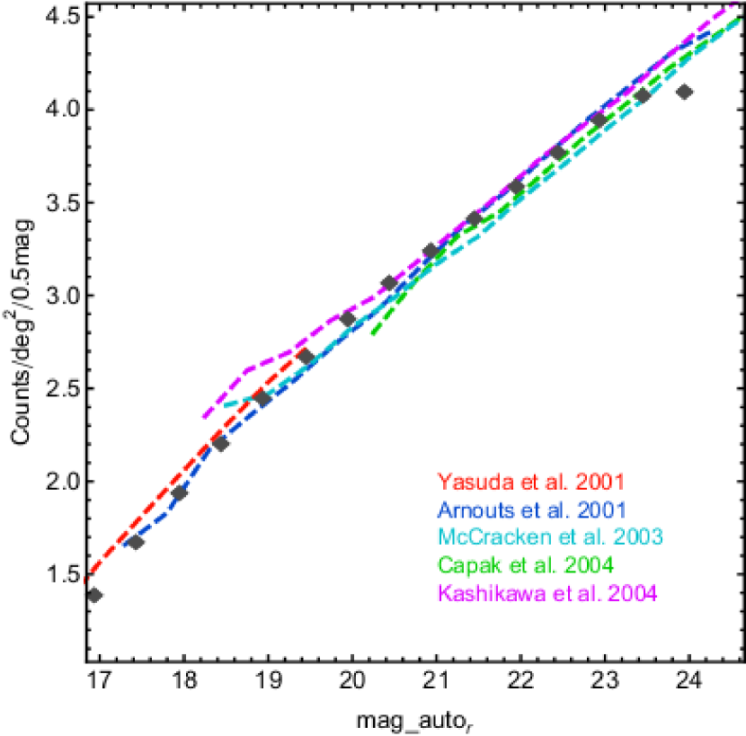
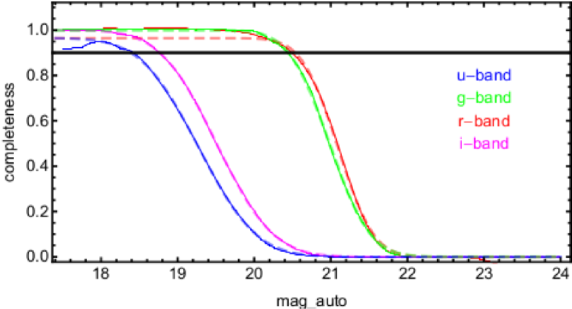
Figure 1: Top: Galaxy counts (grey boxes) as a function of their MAG_AUTO in $r-$band are compared with other literature estimates (as in the legend). The match with previous literature is very good at fainter magnitudes while is not perfect at the brightest ones due to the limited area covered. See also the discussion in the text. Bottom: completeness of the "high $S/N$" sample in $u,~{}g,~{}r$, and $i$-band with colour code as in the legend. The completeness has been computed with respect to the 6 million sample. The derived completeness from data are shown as solid lines, while the best fit using Eq. 1 are plotted as dashed lines

2 Sample Selection

The sample adopted in this analysis consists of galaxies extracted from 153 square degree of the KiDS survey (de Jong et al. 2015) which have been already presented in Tortora et al. (2016). Details about the data reduction and calibration can be found in de Jong et al. (2015). In the following we give a brief summary of the way the galaxy sample has been selected.

Single band source lists for the observed tiles are extracted using a stand-alone procedure named KiDS-CAT, which uses Sextractor (Bertin & Arnouts 1996) for the source detection, star galaxy separation and the catalog extraction. In particular, the star/galaxy (S/G) separation is based on the CLASS_STAR parameter from S-Extractor measured on the $r$-band images, the deepest and best seeing ones for KiDS, following the procedure described in de Jong et al. (2015, Sect. 4.5.1).

While the S/G separation is mainly based on the single $r-$band shape information, source colours are measured based on multi-band source catalogs, which have been obtained using S-Extractor in dual image mode by taking the $r-$band images as reference for source extraction and then measuring the source fluxes in the registered images from the other bands, at the sky position of the $r-$band detection. The fluxes from the multi-band catalog have been used to perform the stellar population synthesis as described in Sect. 2.3. Among the sources selected as galaxies ($\sim$ 11 millions), we have retained those sources which were marked as being out of critical areas from our masking procedure (see de Jong et al. 2015, Sect. 4.4). The effective uncritical area has been found to be $103$ square deg, which finally contains $\sim$6 million galaxies. This latter sample turned out to be complete out to $\sim 24$ mag in $r-$band by comparing the galaxy counts as a function of extinction-corrected MAG_AUTO (used as robust proxy of the total magnitude) with previous literature (e.g. Yasuda et al. 2001, Arnouts et al. 2001, McCracken et al. 2003, Capak et al. 2004, Kashikawa et al. 2004), as shown in Fig. 1.

Finally, in order to perform accurate structural parameter measurement for these systems, we have selected galaxies with “high” signal-to-noise ($S/N$), defined as $1/\mbox{{\tt MAGERR\_AUTO}}$ (Bertin & Arnouts 1996). Specifically, we have used $\mbox{$S/N$}>50$ as initial guess for reliable structural parameters (La Barbera et al. 2008). This choice of $S/N$ will be fully checked by applying the 2D surface brightness fitting procedure (see Sect. 3.1) to mock galaxies in Sect. 3.3.2. We refer to the samples resulting from the $S/N$ selection, as the “high-$S/N$” samples, consisting of 4240, 128906, 348025, and 129061 galaxies, in the $u$, $g$, $r$, and $i$ bands, respectively. These represent the galaxy samples used for the model fitting procedure in the different bands as described in §3. The final output sample to be used for structure parameter analysis will be discussed in §4.1

2.1 Magnitude completeness

The difference in counts among the different bands is due to their intrinsic depth, being the latter a combination of exposure time and seeing, with the $u$-band the shallowest band and the $r$-band the deepest in the KiDS survey plan (see de Jong et al. 2015).

In order to evaluate the completeness magnitude of our sample in different bands, we have computed the fraction of the detected galaxies of the high–$S/N$ sample in bin of $\tt MAG\_AUTO$ with respect to number of galaxies in the same bins of a deeper and complete samples and finally fit the binned fractions with a standard error function model (see e.g. Rykoff et al. 2015).

$${\rm comp}=(1/2)\left[1-erf\left(\frac{m-m_{50}}{\sqrt{2w}}\right)\right],$$ (1)

where $m_{50}$ is the magnitude at which the completeness is 50%, and $w$ is the (Gaussian) width of the rollover. The magnitude at which the sample is 90% complete has been extrapolated by the best fit function. As shown in Fig. 1 (top panel), the full sample of 6 million galaxies detected in the KiDS area has counts consistent with other literature samples and can be used as a reference counts to obtain the fraction of galaxies of the high–$S/N$ sample as shown in the bottom panel of Fig. 1. In this latter plot, we show the interpolated completeness function from the data as solid lines and the best fit curves as dashed lines. The derived 90% completeness limit are 18.4, 20.4, 20.5, and 18.8 for $u$, $g$, $r$, and $i$-band respectively.

2.2 Photometric Redshifts

Photometric redshifts have been derived from Multi Layer Perceptron with Quasi Newton Algorithm (MLPQNA) method (see Brescia et al. 2013; Brescia et al. 2014, Cavuoti et al. 2015a), and fully presented in Cavuoti et al. (2015b), which we address the interested reader for all details. This method makes use of an input knowledge base (KB) consisting of a galaxy sample with both spectroscopic redshifts and multi-band integrated photometry to perform the best mapping between colours and redshift. In particular, we have used 4^′′ and 6^′′ diameter apertures to compute the magnitudes to be used to best perform such a mapping on the training set (see Cavuoti et al. 2015b for more details). While the spectroscopic redshifts for the KB are given by the Sloan Digital Sky Survey data release 9 (SDSS-DR9; Ahn et al. 2012) and Galaxy And Mass Assembly data release 2 (GAMA-DR2; Driver et al. 2011). This sample consists of $\sim 60,000$ galaxies with spectroscopic redshifts out to $z\mathrel{\hbox to0.0pt{\lower 3.5pt\hbox{\hskip 0.5pt$\sim$}\hss}\raise 0.5pt\hbox{$<$}}0.8$, as shown in Fig. 2. $60$ per cent of the sample is used as training set, to train the network, looking at the hidden correlation between colours and redshifts. While the rest of the galaxies in the KB are collected in the blind test set, needed to evaluate the overall performances of the network with a data sample never submitted to the network previously (see right panel in Fig. 2). The scatter in the measurement, defined as $(z_{spec}-z_{phot})/(1+z_{spec})$, is $\sim 0.03$ (see Cavuoti et al. 2015b). The advantage of the machine learning techniques resides in the possibility of optimizing the mapping between the photometry and the spectroscopy regardless the accuracy in the photometric calibration, but the disadvantage consists in the limited applicability of the method only to the volume in the parameter space covered by the KB sample (see Cavuoti et al. 2015b). In our case, for instance, of the 6 millions starting systems, accurate photo-z have been derived for systems down to $r\sim 21$, i.e. $\sim$1.1 million galaxies. This sample is still deeper than the high–$S/N$ sample (see Sect. 2.1). After completing the analysis presented in this paper, new set of machine learning photo-z were made available to the KiDS collaboration (see Bilicki et al. 2017 for details). This will be used for the forthcoming analysis of the next KiDS data releases.

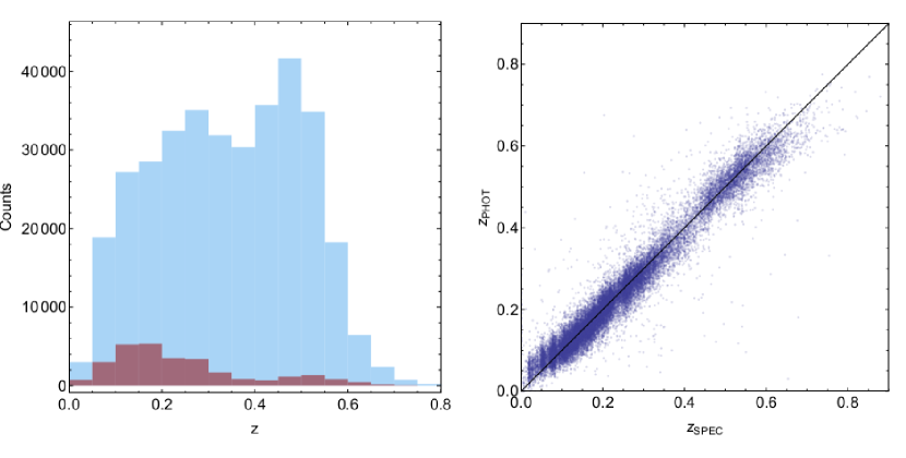
Figure 2: Left: The distribution of the spectroscopic sample adopted as knowledge base for the MLPQNA method (in red) and the photo-$z$ distribution of the “high $S/N$” sample (in light blue). Right: Comparison between spectroscopic and photometric redshifts for the blind test set. See the text for more details.

2.3 Stellar Mass and galaxy classification

Stellar masses, rest-frame luminosities from stellar population synthesis (SPS) models and a galaxy spectral-type classification are obtained by means of the SED fitting with Le Phare software (Arnouts et al. 1999; Ilbert et al. 2006), where the galaxy redshifts have been fixed to the $z_{\rm phot}$ obtained with MLPQNA. We adopt the observed $ugri$ magnitudes (and related $1\,\sigma$ uncertainties) within a $6^{\prime\prime}$ aperture of diameter, which are corrected for Galactic extinction using the map in Schlafly & Finkbeiner (2011).

To determine stellar masses and rest-frame luminosities, we have used single burst SPS models from Bruzual & Charlot (2003) with a Chabrier (2001) IMF. We use a broad set of models with different metallicities ($0.005\leq Z/\mbox{$Z_{\rm\odot}$}\leq 2.5$) and ages ($age\leq\rm age_{\rm max}$), the maximum age, $\rm age_{\rm max}$, is set by the age of the Universe at the redshift of the galaxy, with a maximum value at $z=0$ of $13\,\rm Gyr$. Total magnitudes derived from the Sérsic fitting, $m_{S}$, (see Sect. 3.1) are used to correct the outcomes of Le Phare, i.e. stellar masses and rest-frame luminosities, for missing flux. Typical uncertainties on the stellar masses are of the order of 0.2 dex (maximum errors reaching 0.3 dex).

We have finally used the spectrophotometric classes from Le Phare to derive a classification of our galaxies. As template set for this aim, we adopted the 66 SEDs used for the CFHTLS in Ilbert et al. (2006). The set is based on the four basic templates (Ell, Sbc, Scd, Irr) in Coleman et al. (1980), and starburst models from Kinney et al. (1996). Synthetic models from Bruzual & Charlot (2003) are used to linearly extrapolate this set of templates into ultraviolet and near-infrared. The final set of 66 templates (22 for ellipticals, 17 for Sbc, 12 for Scd, 11 for Im, and 4 for starburst) is obtained by linearly interpolating the original templates, in order to improve the sampling of the redshift-colour space and therefore the accuracy of the SED fitting. We did not account for internal extinction, to limit the number of free parameters.

This fitting procedure provided us with a photometrical galaxy classification, which allows us to separate ETGs (spheroids) from LTGs (disc-dominated galaxies).

2.4 Mass completeness as a function of the redshift

In the following we will study the behaviour of the galaxy properties as a function of the redshift. It is well known that some of the galaxy physical quantities (e.g. size, Sérsic index, colour, etc.) correlate with mass. Hence it is important to define a mass complete sample in each redshift bins.

To do that, we have proceeded in the same way we have computed the completeness magnitudes in Sect. 2.1, i.e. by comparing the high–$S/N$ galaxy counts against the photo-$z$ sample, once galaxies have been separated in different photo-$z$ bins. Results are shown in Fig. 3 and completeness masses are reported in Tab. 1. The table stops at $z=0.6$ because the high–$S/N$sample starts to be fully incomplete in mass above that redshift.

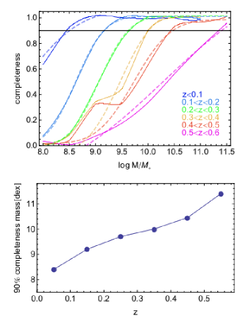
Figure 3: Mass completeness as a function of redshift: the ratio of the high $S/N$ sample and the photo-$z$ sample for galaxies separated in different redshift bins are shown. In the bottom panel the derived completeness from data are shown as dashed lines, while the best fit using Eq. 1 are plotted as solid lines (except for the most massive bin where there was not convergence due to the poor sampling above 90% completeness). The numerical values are reported in Tab. 1. See text for details.

Table 1: 90% completeness mass as a function of the photometric redshift for the high $S/N$ sample.

photo-$z$ bin	90% compl. $\mbox{Log}\ M_{*}/M_{\odot}$
$\leq 0.1$	8.5
$0.1<z\leq 0.2$	9.2
$0.2<z\leq 0.3$	9.6
$0.3<z\leq 0.4$	10.0
$0.4<z\leq 0.5$	10.5
$0.5<z\leq 0.6$	11.4

3 Surface Photometry

In this section we present the measurement of structural parameters for the galaxy sample described above, using 2DPHOT (La Barbera et al. 2008). We evaluate parameter uncertainties and determine the reliability of the fitting procedure using mock galaxy images, with same characteristics as the KiDS images (see Sect. 3.3.2). We finally compare the results obtained with KiDS for galaxies in common with an external catalog from SDSS data (i.e. La Barbera et al. 2010b, Kelvin et al. 2012).

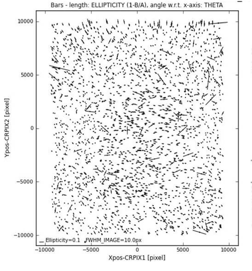
Figure 4: PSF anisotropy within the coadd KIDS_129.0_-0.5 in $r$-band. The elongation is aligned in a specific direction on the borders but random in the middle of the image.

3.1 Structural Parameters

Surface photometry of the high–$S/N$ sample has been performed using 2DPHOT (La Barbera et al. 2008), an automated software environment that allows 2D fitting of the light distribution of galaxies on astronomical images.

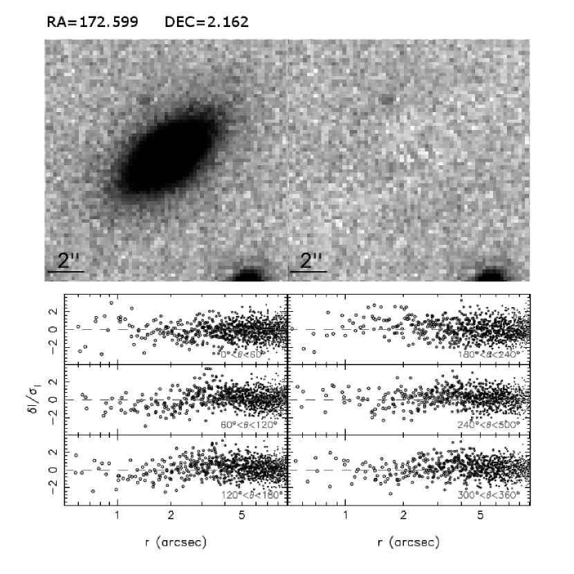
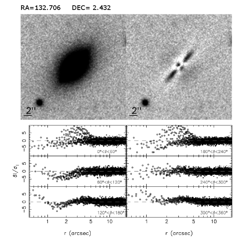
Figure 5: 2DPHOT fitting in $r$-band for two example galaxies with $\chi\prime^{2}<1.3$ (left) and $\chi\prime^{2}>1.3$ (right). In each panel we show the galaxy image (left) and model subtracted image (residual, right). In the six bottom panels, residuals of the galaxy flux per pixel, after the model subtraction, are shown as a function of the distance to the galaxy center, in different bins of the polar angle. See also the text for details.

In particular, 2DPHOT has been optimized to perform a Point Spread Function (PSF) convolved Sérsic modelling of galaxies down to subarcsec scales (La Barbera et al. 2010b). Typical FWHM of KiDS observations are $1.0^{\prime\prime}\pm 0.1^{\prime\prime}$ in $u$-band, $0.9^{\prime\prime}\pm 0.1^{\prime\prime}$ in $g$-band, $0.7^{\prime\prime}\pm 0.1^{\prime\prime}$ in $r$-band, and $0.8^{\prime\prime}\pm 0.2^{\prime\prime}$ in $i$-band (see de Jong et al. 2015, 2017). As usual in large field detectors, the PSF is somehow a strong function of the position across the field-of-view: in Fig. 4 we show a typical PSF pattern in VST/OmegaCAM, images where the solid lines show the amplitude of the elongation and orientation (anisotropy) of the PSF. Especially in the image borders, the orientation of PSFs is strongly aligned, while in the center the PSF tend to be more randomly oriented (isotropic), with smaller elongations. The PSF strongly affects the measurement of the surface brightness profile of galaxies by anisotropically redistributing the light from the inner brighter regions to the outer haloes (see e.g. de Jong 2008), hence altering the inferred galaxy structural parameters (e.g. effective radius, axis ratio, slope of the light profile, etc.). For each source, 2DPHOT automatically selects nearby sure stars and produces average modelled 2D PSF from two or three of them (depending on the distance of the closest stars). The PSF is modelled with two Moffat profiles (see La Barbera et al. 2008). The best-fit parameters are found by $\chi^{2}$ minimization where the function to match with the 2D distribution of the surface brightness values is the convolved function given by

$$\centering M(BG,\{p_{k}\})=BG+B(\{p_{k}\})~{}\rm{o}~{}S\@add@centering$$ (2)

where B is the galaxy brightness distribution, which is described by a set of parameters $\{p_{k}\}$; S is the PSF model; BG is the value of the local background; and the symbol o denotes convolution. The modelled PSF is convolved with a 2D Sérsic profiles with the form

$$\centering B(r,R_{m},n)=I_{0}+\frac{2.5b_{n}}{ln(10)}[(R/R_{m})^{1/n}-1]\@add@centering$$ (3)

For the Sérsic models, the parameters $\{p_{k}\}$ are the effective major semiaxis $R_{m}$, the central surface brightness $I_{0}$, the Sérsic index n, the axial ratio $b/a$, the position angle PA, the coordinates of the photometric center, and the local value of the background. In Fig. 5 two illustrative examples of two-dimensional fit results for galaxies in $r$-band are given. More in details, $R_{\rm e}$ is computed as the circularized radius of the ellipse that encloses half of the total galaxy light, i.e., $\mbox{$R_{\rm e}$}=(b/a)^{1/2}R_{m}$. The total (apparent) magnitude, $m_{T}$, is, by the definition,

$$\centering m_{T}=-2.5\mbox{Log}\ (2\pi)-5\mbox{Log}\ (R_{e})+<\mu>_{e}.\@add@centering$$ (4)

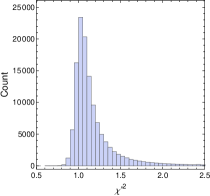
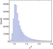
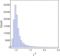
Figure 6: $\chi\prime^{2}$ distribution of galaxies in g, r, and i bands, from left to right.

3.2 Selection of best–fitted data

In order to select the galaxies with most reliable parameters, we defined a further $\chi\prime^{2}$, including in the calculation only the pixels in the central regions. This procedure is different from the standard $\chi^{2}$ definition where the sum of square residuals over all the galaxy stamp image is minimized. The new quantity will provide a better metric to select the galaxies with best fitted parameters as it relies only on pixels with higher $S/N$, while it is not used in the best fitting procedure itself.

To compute the $\chi\prime^{2}$ for each galaxy, all pixels 1$\sigma$ above the local sky value background value are selected and the 2D model intensity value of each pixel is computed from the two dimensional seeing convolved Sérsic model as in Eq. 2. For the selected pixels, the $\chi\prime^{2}$ is computed as the rms of residuals between the galaxy image and the model. The distribution of the $\chi^{\prime 2}$ for the whole high $S/N$ sample in the $g$, $r$, and $i$ bands are given in Fig. 6. As shown in the right panel of Fig. 5 we have galaxies with larger $\chi\prime^{2}$ (e.g. $\chi\prime^{2}>1.3$), which corresponds to lower quality models. This is clearly shown in Fig. 7, which displays more examples of galaxy images and residual maps in the r-band. Here, galaxies with $\chi\prime^{2}<1.3$ are shown on the left two columns and examples of $\chi\prime^{2}>1.3$ galaxies and residuals are on the right two columns. In the first group the Sérsic fit performs very good with almost null residuals, while in the second group substructures like spiral arms, rings, double central peaks from ongoing mergers, etc. show up in the residuals. We substantiate our argument using Fig. 8 where we plot the $n$-index vs. $\chi\prime^{2}$, which shows that for lower Sérsic index ($n<2.5$) there is an excess of large $\chi\prime^{2}$, i.e. worse fit, due the fact that at these low-$n$ late-type systems are predominant (Ravindranath et al. 2002, Trujillo et al. 2007, La Barbera et al. 2002) and tend to have significant substructures. Indeed, the fraction of high $\chi\prime^{2}$ is larger in bluer bands, which is probably affected by star forming regions generally populating substructures of regular discs in late-type systems.

This is a relevant result which show that the good KiDS image quality, combined with an accurate surface photometry analysis, can allow us to correlate the structural properties of the galaxies, as the Sérsic index, with the residuals in the subtracted images, e.g. the typical late-type features. This could provide further parameters for galaxy classification, which we plan to investigate further in future analyses.

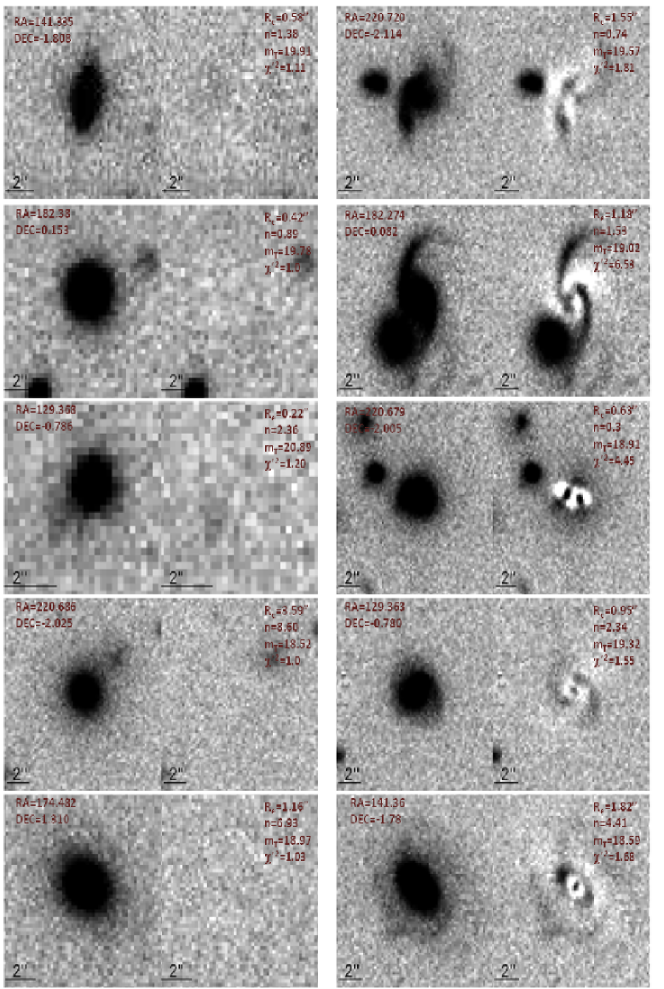
Figure 7: More examples of the 2D fit results for galaxies in r band. The left panels show the results for galaxies with good fits ($\chi\prime^{2}<1.3$) and the right panels those with bad fits ($\chi\prime^{2}>1.3$). In each panel the source and the model subtracted residual maps are shown.

The use of a single Sérsic profile is not the more general choice we could make, as it is well known that galaxies generally host more than one photometric component (see e.g. Kormendy et al. 2009). This is not only true for late-type systems, showing a bulge+disc structure, but also for some large ellipticals, now systematically found to have extended (exponential) haloes (e.g. Iodice et al. 2016). Looking at the $\chi\prime^{2}$ distribution in Fig. 6, the fraction of galaxies with $\chi\prime^{2}>1.3$ is not negligible, and amounts to $\sim 40\%$ in $r$-band.

However, the adoption of multi-component models has two main disadvantages: the degeneracies among parameters and the higher computing time due to the higher dimensionality of the parameter space. In particular, the amount and the quality of the information (e.g. the number of pixels across which typically high$-z$ galaxies are distributed on CCDs of the order of few tens) makes very hard to obtain reliable modelling of multi-component features in galaxies, especially when the ratio between the two components is unbalanced toward one (see e.g. the case in the right panel of Fig. 5, where the inner disc represents a minor component of the dominant bulge).

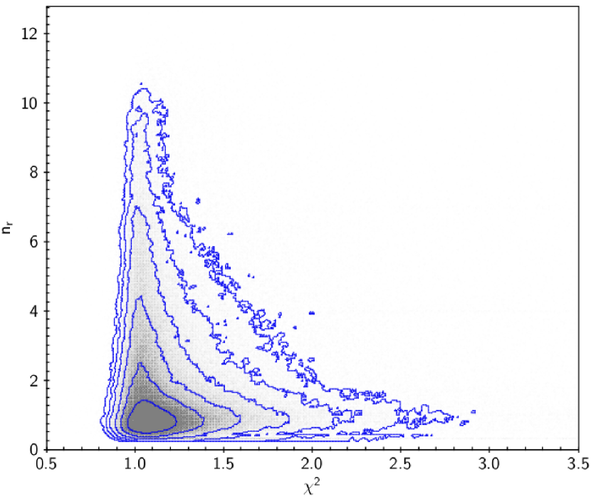
Figure 8: The plot shows the Sérsic index vs. $\chi\prime^{2}$ in $r-$band. We note that at lower $n$ ($\mathrel{\hbox to0.0pt{\lower 3.5pt\hbox{\hskip 0.5pt$\sim$}\hss}\raise 0.5pt\hbox{$<$}}2.5$) there is an excess of large $\chi\prime^{2}$ ($>1.3$), due to the presence of substructures in the residuals, demonstrating that these $n$ values are a good proxy of later morphological types. Log-spaced isodensity contours show that the tails of high-$\chi\prime^{2}$ become dominant in the $\chi\prime^{2}$ distribution of the best-fit at the smaller Sérsic index index (i.e. $\chi\prime^{2}\mathrel{\hbox to0.0pt{\lower 3.5pt\hbox{\hskip 0.5pt$\sim$}\hss}\raise 0.5pt\hbox{$<$}}2$).

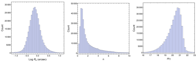
Figure 9: Distribution of structural parameters in r-band: for Log  $R_{\rm e}$, $n$, $m_{T}$, from left to right panel.

For our analysis we have adopted image stamps centered on each galaxy of $\sim$ 100 arcsec by side, i.e. 500 pixels given the resolution of telescope of 0.2 arcsec/pix. This stamp size has been chosen as best compromise between computational speed and area covered. We have excluded from our analysis galaxies with $\mbox{$R_{\rm e}$}>50^{\prime\prime}$, as these might be (i) galaxies for which the 2D light distribution is poorly sampled, resulting into overly large $R_{\rm e}$ values or (ii) galaxies with a second extended component, that is modelled as a single component with large $n$, resulting into large $R_{\rm e}$. We conclude this section by showing the distribution of the best-fit structural parameters obtained in $r$-band to give a perspective of the parameter space covered by the sample. In Fig. 9 this is given for the effective (half-light) radius, $R_{\rm e}$, the Sérsic index, $n$, and the total magnitude, $m_{T}$. The median effective radius of the sample is 5.4 arcsec, while the median of the Sérsic index is 1.3 and the median of the total mag is 20.4 in $r$-band. The distribution of the $R_{e}$ is quite symmetric and show that we can reach galaxy sizes of the order of the tenths of the arcsec for the smallest systems, while the largest galaxies measured can be as large as 10 arcsec and more. The Sérsic index distribution shows a large tail toward the larger n-index, i.e. at $n>2$. This shows that the spheroidal-like systems are not the dominant class of galaxies in our sample. The total magnitude distribution also shows the effect of the sample completeness as the median almost corresponds to the completeness magnitude (see §2.1).

3.3 Uncertainties on structural parameters

We have estimated the statistical errors on the estimated structural parameters using two approaches: 1) internal: by comparing estimates obtained by or best fit in contiguous bands; 2) simulations: by applying our procedure on mock galaxies mimicking KiDS observations and checking how the estimated parameters compare to the know input ones of the simulated galaxies.

3.3.1 Internal check

We first estimate the uncertainties on structural parameters by comparing the differences in Log  $R_{\rm e}$, $\langle\mu_{e}\rangle$, and $\mbox{Log}\ n$ between contiguous wavebands, in our case we have adopted $r$ and $i$ bands. The basic assumption is that these two bands are close enough that the variation of the galaxy properties from one band to other is dominated by the measurement errors (La Barbera et al. 2010b). Therefore, this approach provides an upper limit to the uncertainty on structural parameters.

For the uncertainty calculation we follow the method explained in La Barbera et al. (2010b). We bin the differences in the Log  $R_{\rm e}$, $\langle\mu_{e}\rangle$, and $\mbox{Log}\ n$ between $r$ and $i$ bands with respect to the Logarithm of the mean effective radius Log  $R_{\rm e}$ and $S/N$ per unit area of the galaxy image, $\mbox{$S/N$}/{R_{e}}^{2}$. In this case the $S/N$ is defined as the mean value of the inverse of MAGERR_AUTO, between the two bands. Bins are made such that the number of galaxies in each bin is same. Measurement errors on Log  $R_{\rm e}$, $\langle\mu_{e}\rangle$, and $\mbox{Log}\ n$ are computed from the mean absolute deviation of the corresponding differences in that bin. The results are shown in Fig 10.

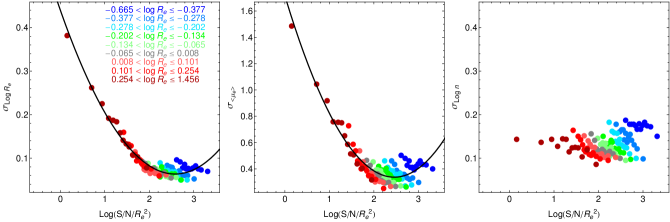
Figure 10: Uncertainties in the parameters Log  $R_{\rm e}$, $\langle\mu_{e}\rangle$, and $\mbox{Log}\ n$ as a function of the Logarithm of the $S/N$ per unit area. Different colours show different bins of Log  $R_{\rm e}$, where $R_{\rm e}$ is in arcsec. For a given colour the points are the uncertainties in different bins of Logarithm of $S/N/\mbox{$R_{\rm e}$}^{2}$. The black curve is the best fitting functional form used to model the dependence of the uncertainties on S/N. This fit is not performed for $\mbox{Log}\ n$ as it does not shows any correlation with S/N$/\mbox{$R_{\rm e}$}^{2}$.

The errors on the parameters show a dependency on the S/N per unit area: as the value of S/N per area decreases ($\mbox{Log}\ (S/N/\mbox{$R_{\rm e}$}^{2})<2$), the errors tends to increase. This is due to the combined effect of the S/N and the number of pixels where the signal is distributed. At low $S/N/{\mbox{$R_{\rm e}$}}^{2}$, there are sources with large $R_{\rm e}$ and small S/N, whereas high $S/N/{R_{e}}^{2}$ are systems that might have large S/N, but due to the small number of pixels induces the uncertainty on parameters. Most of the galaxies have $R_{\rm e}$ in the range $-0.5<\mbox{Log}\ \mbox{$R_{\rm e}$}<0.2$, where the errors on the parameters are less than 0.1 dex for $R_{\rm e}$ and less than 0.4 dex for $\langle\mu_{e}\rangle$, but the errors on $n$ are more randomly distributed and do not show particular trends. However, also in this case, they stay remarkably contained below 0.2 dex.

3.3.2 Simulated galaxies

A further approach to assess the reliability of the parameters obtained from the fitting procedure and estimate their intrinsic statistical errors, is based on mock galaxy images generated on top of a gaussian background noise, given by the background rms measured for the KiDS images. The artificial galaxies have physical parameters, i.e., magnitude, Sérsic index, effective radius, and axis ratio, which are assigned based on a grid of values. For each parameter, the grid of values was chosen based on the range of values for the observed galaxies. In particular we have uniformly sampled the parameters in the following intervals: $0.2\leq\mbox{$R_{\rm e}$}\leq 20$ arcsec, $0.6\leq n\leq 10$, $0.5\leq b/a\leq 1$, and $16\leq m_{T}\leq 24$ mag. About the choice of using a uniform distribution in total magnitude, instead of using a realistic luminosity function, we stress here that we are not interested in producing realistic images, but rather realistic individual systems which we want to analyse to assess the robustness of our procedures. This causes a lack of faint systems in our simulated images with respect to real images as seen in Fig. 11. As this does not impact the local background of the brighter systems, representative our complete sample, the overall results of the analysis are not affected. We have simulated about 1800 galaxies on image chunks of 3000 pixels by side in order to reproduce the same galaxy density observed in KiDS images. We have generated such mock observations in different bands and in different seeing conditions. In Fig. 11 we show an example of simulated $r$-band image, compared with a real one.

We have then applied 2DPHOT to the mock images with the same setup used for the real images (see Sect. 3). The relative differences between the measured quantities and the input ones adopted to generate the simulated galaxies are shown in Fig. 12 as a function of the $S/N$.

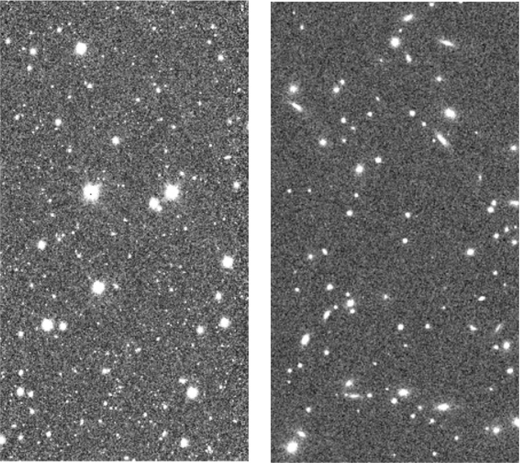
Figure 11: A real KiDS image (left) vs. a mock image with simulated galaxies (right). Seeing FWHM are 0.69 and 0.66 for real and mock images respectively.

The figure shows that the input and output values are well in agreement with each another, except in the low-$S/N$ regime (i.e., $S/N\mathrel{\hbox to0.0pt{\lower 3.5pt\hbox{\hskip 0.5pt$\sim$}\hss}\raise 0.5pt\hbox{$<$}}50$), where we start observing a systematic deviation of the measured values from the input ones. This is an a posteriori confirmation that our choice of $\mbox{$S/N$}>50$ for robust structural parameter studies was correct.

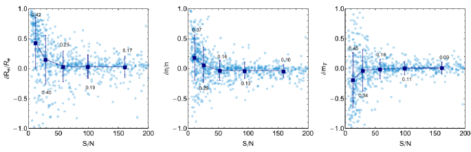
Figure 12: Figure shows differences between the input and output parameters for $R_{\rm e}$  n, and $m_{T}$, with respect to $S/N$. We define the quantity $\delta p_{k}=(p_{k}^{\rm in}-p_{k}^{\rm out})$, with $p_{k}=\mbox{$R_{\rm e}$}\,~{}n,~{}m_{T}$. We plot $\delta\mbox{$R_{\rm e}$}/\mbox{$R_{\rm e}$}^{in}$, $\delta n/n^{in}$ and $\delta m_{T}$ in terms of $S/N$. Datapoints for single galaxies are plotted as blue points. Mean values are plotted as filled squares and error bars show the standard deviation in bins of $S/N$. The numbers given are the standard deviations in each bin.

In the same Figure we show the relative differences of the same observables against the input values (bottom row): in this case there is no trend in the derived quantities and statistical errors stay always below 10%. We have found that these good accuracies are independent of the band and of the seeing, as long as we restrict to galaxies with $\mbox{$S/N$}>50$ in any given bands.

3.4 Check for systematics on the estimated parameters

In this section we proceed with a series of validation tests to check the presence of biases in the parameter estimates. To do that we have selected literature samples having an overlap with our KiDS galaxy sample. However, before going on with tests on external catalogs we will start with a basic check on the effect of the background evaluation on the parameter estimates.

3.4.1 Effect of sky background

We have discussed in Sect. 3.1 that the background is a free parameter in our fitting procedure (see e.g. Eq. 2). However, it is well known that the simultaneous fit of the background and the photometric laws can be degenerate and produce some systematics.

In order to estimate the effect of background fitting on the estimate of structural parameters, we have repeated the fitting of galaxy image by keeping the background as a fixed parameter. We measured the background value far from the galaxy (local background value calculated from the galaxy stamp images, which is 1.5 times the S-Extractor $ISOAREA$ parameter, see La Barbera et al. 2008 for more details) and entered as the initial guess in the fitting procedure. Here, we fix this value of background for the modelling.

We randomly selected $\sim$ 3000 galaxies from our high–S/N galaxy sample and again extracted the structural parameters. We compare the two sets of structural parameters we have obtained with the standard procedure and the one with fixed background. The differences in structural parameters are shown in Fig. 13.

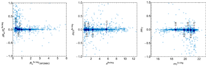
Figure 13: Differences in the $r$-band parameters $R_{\rm e}$  n, and magnitude when background is kept constant with respect to the value when background is subjected to change. We define the quantity $\delta p_{k}=(p_{k}^{\rm fix}-p_{k}^{\rm var})$, with $p_{k}=\mbox{$R_{\rm e}$}\,~{}n,~{}m_{T}$. We plot $\delta\mbox{$R_{\rm e}$}/\mbox{$R_{\rm e}$}^{fix}$, $\delta n/n^{fix}$ and $\delta m_{T}$ as a function of $\mbox{$R_{\rm e}$}^{fix}$, $n^{fix}$ and $m_{T}^{fix}$, respectively. Mean values are plotted as filled squares and are given along with the single datapoints. Error bars show the standard deviation in bins of parameter plotted on x axis. The numbers given are the standard deviation in each bin.

Squares and error bars represent mean and standard deviation of the scattered plot. For most of the selected galaxies the differences between measured and input parameters are negligible. The background fit does not introduce systematics and the error associated to the background measurement is of the order of 10-20% in $R_{\rm e}$  less than 10% in $n$, and less then 20% in the total magnitude, which are in line with the estimates in Sect. 3.3.

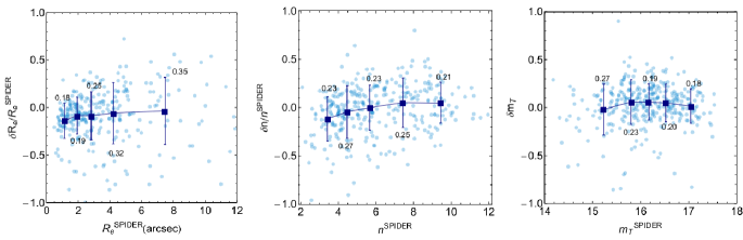
Figure 14: Comparison of KiDS structural parameters with the ones derived within the SPIDER survey. The SPIDER dataset consists of spheroids with redshifts in the range $0.05<z<0.095$, selected from SDSS; the structural parameters are derived using 2DPHOT. We define the quantity $\delta p_{k}=(p_{k}^{\rm SPIDER}-p_{k}^{\rm KiDS})$, with $p_{k}=\mbox{$R_{\rm e}$},~{}n,~{}m_{T}$. We plot $\delta\mbox{$R_{\rm e}$}/\mbox{$R_{\rm e}$}^{SPIDER}$, $\delta n/n^{SPIDER}$ and $\delta m_{T}$ in terms of $R_{\rm e}$, n and $m_{T}$, respectively. Data are shown as points. Mean values and standard deviations are plotted as filled squares and error bars. The numbers are the standard deviations in each bin.

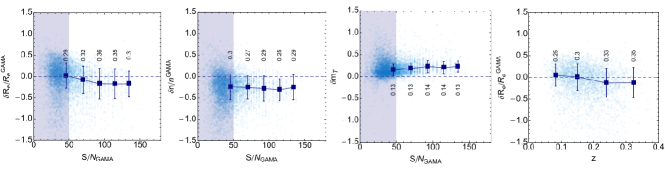
Figure 15: Comparison of KiDS structural parameters with the ones derived by GAMA using SDSS images (Kelvin et al. 2012). The structural parameters are derived using GALFIT (Peng et al. 2002). We define the quantity $\delta p_{k}=(p_{k}^{\rm GAMA}-p_{k}^{\rm KiDS})$, with $p_{k}=\mbox{$R_{\rm e}$},~{}n,~{}m_{T}$. In the first three panels we plot $\delta\mbox{$R_{\rm e}$}/\mbox{$R_{\rm e}$}^{GAMA}$, $\delta n/n^{GAMA}$ and $\delta m_{T}$ as a function of $S/N$. In the fourth panel to the right, we also plot the $\delta\mbox{$R_{\rm e}$}/\mbox{$R_{\rm e}$}^{GAMA}$ vs. redshift, which shows that there is no significant systematics between the GALFIT parameters and the ones obtained with 2DPHOT as a function of the redshift. Median values and median deviations divided by 0.675 (as equivalent to the standard deviation) are plotted as filled squares and error bars. The numbers are the standard deviations in each bin.

3.4.2 Comparison of KiDS and SDSS structural parameters

We want now to compare our results with some external catalogs to check the presence of biases. The accuracy of our structural parameter estimates is compared with two samples which overlaps with KiDS sky area.

First, the SPIDER galaxies (La Barbera et al. 2010b), which includes 39,993 spheroids with SDSS optical imaging and UKIDSS Near Infra Red (NIR) imaging, with redshifts in the range $0.05\mathrel{\hbox to0.0pt{\lower 3.5pt\hbox{\hskip 0.5pt$\sim$}\hss}\raise 0.5pt\hbox{$<$}}z\mathrel{\hbox to0.0pt{\lower 3.5pt\hbox{\hskip 0.5pt$\sim$}\hss}\raise 0.5pt\hbox{$<$}}0.1$.

This sample has structural parameters derived with the same software (2DPHOT) used in this paper for KiDS, but applied on SDSS images, which have a poorer image quality. This would give us the effect of depth (KiDS is two magnitudes deeper than SDSS) and image quality (both pixel scale and seeing are about twice smaller in KiDS) on the parameter estimates being the analysis tool substantially the same for the two datasets. By matching the KiDS data with SPIDER we found 344 galaxies in common for which we can have a direct comparison of the derived parameters. This allows us to measure the relative differences among the structural parameters. The results are shown in Fig. 14, where we can see a good agreement among the parameters from the two datasets with the scatter (measured by the errorbars) in line with the statistical errors ($\sim$10% or below) discussed in Sect. 3.3.2.

Secondly, we have checked our structural parameters with the ones obtained by the GAMA collaboration (Kelvin et al. 2012) using GALFIT (Peng et al. 2002) on SDSS optical images. This subsample consists of 7857 galaxies and the results are shown in Fig. 15, where again we plot the relative differences among the structural parameters. In this test, both data and analysis methods are different, hence we can check whether the combination of the image quality and the analysis set-up can introduce some differences in the galaxy inferences.

The comparison with SDSS and KiDS data shows a clear offset between the two sets of parameters of the order of 20%. This was already found when comparing the 2DPHOT estimates with GALFIT on SDSS data (see e.g. La Barbera et al. 2010b for details), hence this has to be related to the different tools’ performances. In Fig. 15 we plot the structural parameters against the $S/N$ defined as for the KiDS case. We can see that a large part of the GAMA sample have a $S/N$$<50$, a region where the scatter among the two analysis increases and results from SDSS should be less robust. However, the offset shows-up at the higher $S/N$ which suggests that the differences are not due to the poorer SDSS quality. In general, effective radii and Sérsic indices with GALFIT are smaller with respect to those of 2DPHOT by 15% and 25% or less respectively, whereas the total magnitude from 2DPHOT is brighter by $\sim 0.2$ mag compared to the SDSS. The offset of the $R_{\rm e}$  in particular, seems consistent with zero within the (albeit large) scatter.

There might be many reasons why the two software might have brought to systematics (e.g. PSF sampling, convolution methods, background estimate etc.) and a detailed discussion of the origin of this is beyond the scope of this paper. Based on our test done with mock galaxies in Sect. 3.3.2, corroborated by the check vs. the SPIDER sample, we are confident that the 2DPHOT estimates are fairly accurate. However, we will perform a challenge of different surface photometry tools on an advanced mock galaxy catalog on the next paper (Raj et al., in preparation). We just remark here that there seems to be no trend of the offset with the redshift, as shown on the last panel of Fig. 15: since most of the focus of the paper is on the galaxy size evolution with redshift, we believe that our results should not suffer any severe systematics.

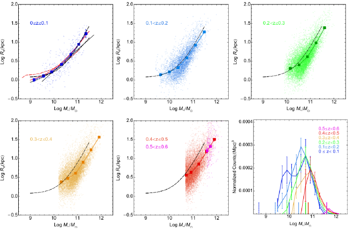
Figure 16: Size–Mass relation for spheroids (top panels and left and central bottom panels). Individual galaxy values are plotted together with mean and standard deviation of the mean (boxes and error bars). For the $0\leq z<0.1$ bin we overplot some local relations from literature (solid line: Shen et al. 2003; dot-dashed line: Hyde & Bernardi 2009; dashed black line: Mosleh et al. 2013; dashed red line: Baldry et al. 2012; solid red line: Lange et al. 2015). For all other $z$ bins we show the $z=0$ relation form Mosleh et al. (2013) to visually appreciate the deviation of the average relation from the local one. Bottom right panel: the stellar mass distributions in different $z$ bins normalized to the total covolume. The vertical coloured line at the bottom of the bottom-right panel are the rough mass completeness derived by the histogram shown in the same panel. Here we took as fiducial completeness mass the mass roughly corresponding to the peak of the distribution, except for the lowest z bin where we also keep the second peak of the mass distribution as a significant feature.

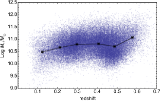
Figure 17: Mass vs. redshift plot for the spheroids sample. Overplotted to the individual galaxy values, we show the mean and standard deviation of the mean of the sample (error bars are comparable to the size of the boxes). Note that the steepening of the $z\sim 0.6$ bin is due to the mass incompleteness of this bin. In the lowest $z$ bin ($z\sim 0.1$), the sample suffers some volume incompleteness (see discussion in Sect. 2), which produces the mean mass in the bin to be biased toward less massive systems.

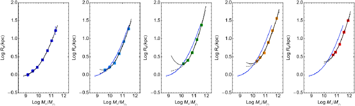
Figure 18: Parametric fit to the Size–Mass relation for spheroids. The average size mass in different bins (colour coded as in Fig. 16) is fitted with the parametric formulae as in Eqs. 5 (dotted lines) and 6 (solid lines). The $z=0$ fit has been reported in the subsequent $z$ bins in blue, to visually check the difference of the $z>0.1$ relations. These curves are used to define the $R_{\rm e}$ corresponding to different mass intercepts as shown in Fig. 19.

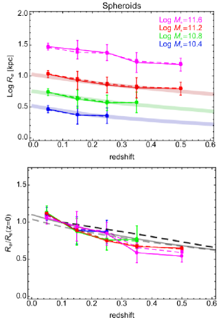
Figure 19: Size vs. $z$ plots from the average size-mass parametric fit of spheroids. Top. We plot the derived absolute intercept of the best fit relations as in Fig. 18 at mass values in the legends. Error bars account for the $1\sigma$ errors in the best fit. Dotted and solid lines show the results of fit from the M+13 relations as in Eq. 5 and HB+09 relation as in Eq. 6 respectively. We also overplot results from HST data in vdW+14, corresponding to $\mbox{Log}\ M_{*}/M_{\odot}=10.25,~{}10.75,~{}11.25$, from bottom to the top, which well compare to our measurements in similar mass bins. Bottom. We plot the size evolution with respect to the local size at different mass intercepts. The evolution of the size with redshift becomes increasingly significant at larger masses. The black dashed line is the relation as found by Trujillo et al. (2007) for $\mbox{Log}\ M_{*}/M_{\odot}>11.0$. The grey dashed line is for ETGs with $10.5<\mbox{Log}\ M_{*}/M_{\odot}<11.0$ and the grey solid line for those with $11.2<\mbox{Log}\ M_{*}/M_{\odot}<12$ from Huertas-Company et al. (2013).

4 Results

In this section we present results about the evolution across cosmic time of galaxy sizes and size–mass relations. The evolution of the size–mass correlation is strictly related to the way the galaxies have been assembled. It is known that the two main classes of galaxies, spheroids and disc-dominated, show a different dependency between size and stellar mass with disc-dominated galaxies having a weak, if any, dependence on the redshift, and spheroids showing a clear variation with the redshift (see e.g. Shen et al. 2003, van der Wel et al. 2014), which suggest a different evolution pattern for the two populations. In the following, we will refer to effective radii derived in $r$-band if not otherwise specified.

4.1 Spheroids and disc-dominated galaxy classification

We start by separating spheroids and disc-dominated galaxies using two independent criteria, based on: a) the Sérsic index values (Sect. 3) and b) the SED fitting classification using the spectrophotometric classes discussed in Sect. 2.3. We define "spheroids" those systems with steep light profiles, i.e. with $r$-band $n>2.5$ (Trujillo et al. 2007, van der Wel et al. 2014), and with photometry best-fitted by one of the 22 elliptical galaxy model templates (see Sect. 2.3; Tortora et al. 2016). Instead, "disc-dominated" galaxies are defined as systems with more extended and shallower light profiles, i.e. with $r$-band $n<2.5$, and with photometry which is best-fitted by model templates of late-type galaxies (i.e., Sbc and Scd types).

The final sample consists of $49\,972$ spheroids and $144\,859$ disc-dominated galaxies in $r$-band. We just remark that there are a number of galaxies ($13\,403$) which turned out to be neither spheroids nor disc-dominated (classified as star burst or irregular systems), which we have excluded from our analysis. Furthermore, in order to use with caution the warning of the offset found with the GAMA estimate in §3.4.2, we show that our results are insensitive to a more conservative choice of the Sérsic-index (e.g. adopting $n>3.5$) in Appendix C.

4.2 Size–Mass as a function of redshift

Once we have defined the two main galaxy classes interested by this analysis, we can proceed to investigate the size–mass relation as a function of the redshift and compare this with previous literature data and simulations.

4.2.1 Spheroids

In Fig. 16 we show the size–mass relation of spheroids in different redshift bins with overplotted the mean as boxes and the standard deviation of the mean as errorbars. In Fig. 16 only the 90% complete sample is shown, and this becomes clear in particular at $z>0.3$ where the sample starts to be severely incomplete at $\mbox{Log}\ M_{*}/M_{\odot}<10.2$. The two bins at $z>0.4$ are shown together as the contribution of galaxies in the bin $0.5<z\leq 0.6$ is minimal and limited to the very high mass end. The mean contour of the latter redshift bins are fully consistent with the ones derived for the lower z bin, $0.4<z\leq 0.5$, hence we decided to cumulate the two samples.

In the figure we have also plotted some relevant literature trends obtained at $z=0$ (i.e. Shen et al. 2003, S+03 hereafter; Hyde & Bernardi 2009, HB+09 hereafter; Mosleh et al. 2013, M+13 hereafter; Baldry et al. 2012, B+12 hereafter; Kelvin et al. 2012, K+12 hereafter; Lange et al. 2015, L+15 hereafter), after having scaled all masses to the Chabrier IMF, which is our reference choice. All the literature results used for comparison had been obtained with a single Sérsic model (as for our results) except for HB+09 which used a simple de Vaucoleurs profile. Also, we had to take into account the different size definitions as circularized radii (i.e. the ones adopted by us) were used by Shen+03, HB+09, and M+13, while B+12, K+12 and L+15 adopted major axis effective radii and needed to be corrected by the galaxy axis ratio (see §3.1). Since we did not have information on the axis ratio of all literature samples, we have adopted an average correction between the major axis and the circularized radii as a function of the mass for the low-$z$ bin obtained from our galaxy sample as discussed in Appendix B (and shown in Fig. 25), which we have applied to the datasets adopting major axis effective radii (i.e. B+12 and K+12). This corresponds to have compared our major axis estimates with the equivalent ones in B+12 and K+12, and then re-arranged all back to some circularized radii consistent with the same average ellipticity of the KiDS galaxies.

We first remark a very good agreement of our mean values (data points with error bars) with the non-parametric estimates from M+13 shown as dashed line in Fig. 16. In particular, we clearly see in our data a flattening of the relation at masses below $\mbox{Log}\ M_{*}/M_{\odot}\sim 10.0$ in the lowest $z$ bin. The $z=0$ relation from M+13 nicely matches also the average trend in our next $z$ bin ($0.1<z\leq 0.2$), where the flattening of the relation is even more evident.

Differently from M+13, S+03 use a single power-law to best fit their data, i.e. $\mbox{$R_{\rm e}$}\propto M^{\alpha}$, while HB+09 have performed a parabolic fit in the Log-Log plane to reproduce the curvature they have observed in their data too and that is also seen in our Fig. 16. Both S+03 and HB+09 show a good agreement with our data at the intermediate mass scales, while they diverge at the lower masses. In particular, S+03 does not seem to catch the flattening of the average size-mass relation, while HB+09 seems to over-predict the flattening we also observe. We expect to better quantify this tension at lower mass scales by using the larger dataset to be gathered with the third data release. We note, though, that the sample is complete at this mass bin according to Tab. 1. At higher masses ($\mbox{Log}\ M_{*}/M_{\odot}>10.8$), the main issue of the S+03 relation, is that they tend to underestimate $R_{\rm e}$ because of sky subtraction in the SDSS Photo pipeline. To conclude our comparison with previous literature, we also show the average relation obtained by Baldry et al. (2012) with GAMA galaxies, where we see also a flattening of the relation at $\mbox{Log}\ M_{*}/M_{\odot}\sim 10.0$, but the overall relation seems tilted with respect to our average relation.

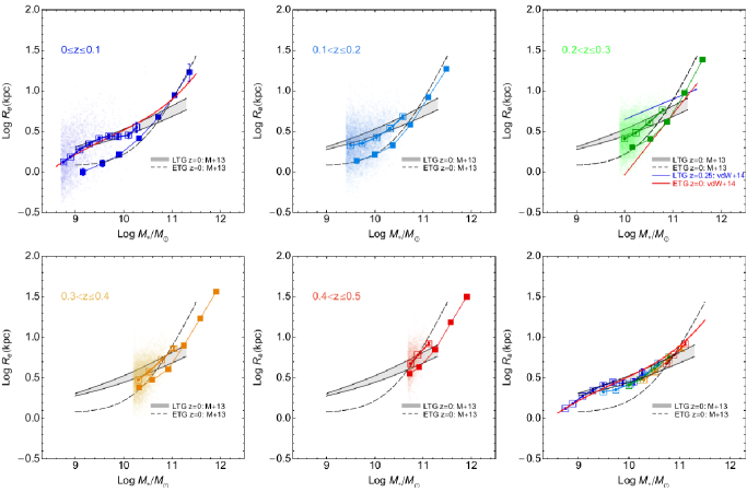
Figure 20: Size–Mass relation for disc-dominated galaxies. Symbols have the same meaning of the spheroids sample in Fig. 16, but now data are shown with open symbols in contrast to the spheroids average relation also shown as full symbols. The local relation is given by a shaded area which show the range spanned by the average relation from Mosleh et al. (2013) (i.e. their LTG, $n<2.5$, blue samples) and solid red line from (Lange et al., 2015). In the bottom right panel we summarize all results: the disc-dominated galaxies have generally larger sizes at masses, especially for $\mathrel{\hbox to0.0pt{\lower 3.5pt\hbox{\hskip 0.5pt$\sim$}\hss}\raise 0.5pt\hbox{$<$}}10^{11.0}M_{\odot}$ and show a trend with redshift (see Sect. 4.2.1) which seems weak or absent.

We use the M+13 results as a $z=0$ reference to compare the size-mass relations in the other redshift bins and visually evaluate the evolution of the size–mass relation with lookback time. Going toward higher $z$, in Fig. 16 we show that the mean correlation (boxes connected by the solid lines) starts to deviate from the $z=0$ relation after $z=0.2$ as galaxies become more and more compact with respect to their low-z counterparts. The difference is significant within the errors at stellar masses $\mbox{Log}\ M_{*}/M_{\odot}~{}\hbox to0.0pt{$>$\hss}{\lower 4.30554pt\hbox{$\sim$}}10.5$, while at lower masses there is little evolution in size, or even, an opposite trend with respect to that seen in the high mass regime, i.e. galaxy sizes becoming larger. However, this might be due to the fact that we are in a mass regime ($M\sim 10^{10}M_{\odot}$) close to the completeness limit of the sample.

On the higher mass side, the sample does not suffer any particular incompleteness, as shown by the mass distribution in the $z$-bins in the bottom-right panel of the same Fig. 16 (except possibly for the low-$z$ bin, see also below). Here, the counts have been normalized to comoving volume and corrected by the completeness function (i.e. the fraction of galaxy lost per mass unit in different $z$-bins). The error bars mainly reflects the propagation of photo-$z$ errors on the determination of the comoving volume in the different $z$-bins. The drop of the counts after the first peak at $\mbox{Log}\ M_{*}/M_{\odot}=10.5-11.0$ going towards lower masses, is typical of the spheroids mass function measured at all redshifts (see e.g. Kelvin et al. 2014) and does not reflect an intrinsic incompleteness of the sample. We conclude that the observed trend with $z$ relation, which moves the spheroids sample progressively away from the $z=0$, is genuine and has to be related to an evolution pattern in the galaxy structural parameters. All these effects go in the sense of favoring more and more massive (hence larger) galaxies at higher $z$, which goes in the opposite direction as the trend of galaxy sizes decreasing with z.

This should not be due to an evolution of the stellar mass, as the average stellar mass of our sample does not show any significant trend with the redshift. This is demonstrated in Fig. 17, where the average masses stay almost constant in the range $\mbox{Log}\ M_{*}/M_{\odot}\sim 10.7-10.8$ as a function of $z$ although a steepening is observed only at the $z\sim 0.6$ bin, which is due to the mass incompleteness of this bin (below $\mbox{Log}\ M_{*}/M_{\odot}=11.5$). A possible selection effect is also present in the lowest $z$ bin ($z\sim 0.1$), due to the volume incompleteness discussed in Sect. 2), which causes the average mass in the bin to be biased toward the less massive systems.

We conclude that the the driver of the evolution of the mass-size relation is the change of the galaxy size with $z$. Visually, this means that galaxies more massive than $\mbox{Log}\ M_{*}/M_{\odot}\sim 10.5$ have sizes (i.e. $R_{\rm e}$) that decrease with increasing redshift at any given mass. To better quantify this effect and to estimate also the amount of the size variation in the different mass intervals, we have performed a fit to the average size–mass at different redshifts and then evaluated the $R_{\rm e}$ corresponding to different mass intercepts (see also van der Wel et al. 2014, hereafter vdW+14).

To fit the size–mass we have used the two fitting formula used in M+13 and HB+09 (as showed in Fig. 16), which we report here below for clarity:

$$\mbox{$R_{\rm e}$}=\gamma(M_{*})^{\alpha}(1+M_{*}/M_{0})^{(\beta-\alpha)}~{}{\rm[from~{}M+13]},$$ (5)

where $R_{\rm e}$ is in kpc, $M_{*}$ in solar units, and $\alpha$, $\beta$, $\gamma$, $M_{0}$ are free parameters, and

$$Y=p_{0}+p_{1}X+p_{2}X^{2}~{}{\rm[from~{}HB+09]}$$ (6)

where $Y=\mbox{Log}\ \mbox{$R_{\rm e}$}{\rm/kpc}$, $X=\mbox{Log}\ M_{*}/M_{\odot}$ and $p_{0},~{}p_{1},~{}p_{3}$ are free parameters to be adjusted to best fit the data points. The best fit relations for both cases are shown in Fig. 18. The fit is generally very good for both fitting function across the data points, however Eq. 6 seems to predict a very strong up-turn of the trend at low masses, right outside the first datapoint, which we cannot confirm with our current dataset.

In Fig. 19 we show the trend of the $R_{\rm e}$, obtained from Eq. 5 and 6, for different mass values, as a function of $z$, while errorbars show errors from the best fit at every mass bin for Eq. 5 only, for clarity (being the ones of Eq. 6 very similar). The errors on the individual estimate take into account the $1\sigma$ errors in the best fit. There is an evident trend of the sizes to decrease with redshift in all mass values except $\mbox{Log}\ M_{*}/M_{\odot}=10.4$. This trend is nicely consistent with a similar analysis performed by vdW+14 on HST data for CANDELS (Koekemoer et al. 2011) and shown in the same figure, where we show their results for $\mbox{Log}\ M_{*}/M_{\odot}=10.25,~{}10.75,~{}11.25$, from bottom to the top (see also the colour code, as in the legenda). Our results are consistent CANDELS at higher-$z$ (>0.3) for the lowest mass value for which our sample is complete out to $z\sim 0.5$ ($\mbox{Log}\ M_{*}/M_{\odot}=10.4$).

If we use the standard parametrization for the size evolution vs. redshift of the form

$$\mbox{$R_{\rm e}$}=B_{z}(1+z)^{\beta_{z}}$$ (7)

we note that the steepest variation of the sizes is found in our highest mass intercept ($\mbox{Log}\ M_{*}/M_{\odot}=11.6$), for which we measure a slope of $\beta_{z}=-2.0\pm 0.3$ as in Tab. 2, where we report the best fit to the data point obtained from Eq. 5 (but the use of Eq. 6 would not have changed the final results). This is different from the ones of the lower mass bins which have an average slope of -1.5, which is consistent with the one reported by vdW+14 (i.e. -1.48). This corresponds to a reduction of the size with respect to the value at $z=0.1$ of galaxies with mass $\mbox{Log}\ M_{*}/M_{\odot}=11.6$ that reaches about 50% at z > 0.5 and that is larger than the 40% of the galaxies of the close mass bin ($\mbox{Log}\ M_{*}/M_{\odot}=11.2$), as shown in the bottom panel of Fig. 19. We used the $z=0.1$ value as normalization value, consistently with previous literature (Trujillo et al. 2007, Huertas-Company et al. 2013) also shown in the figure as comparison.

The evolution of the galaxy size over cosmic time becomes increasingly significant at larger masses. We could not track back these discrepancies in the $\mbox{$R_{\rm e}$}(z)/\mbox{$R_{\rm e}$}(z=0)$ in the original samples from the two analyses mentioned above as the galaxy selection are somehow different from ours (e.g. Trujillo et al. 2007 use systems with $n>2.5$, Huertas-Company et al. 2013 distinguish group and field galaxies) and also the local values adopted by them are different.

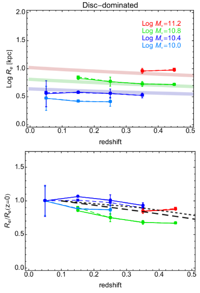
Figure 21: Size vs. $z$ plots from the average size-mass parametric fit of disc-dominated galaxies, as done for spheroids in Fig. 19. Top. We plot the derived absolute intercept of the best fit relations at mass values as in the legend. Dotted and solid lines show the results of fit from the M+13 relations as in Eq. 5 and HB+09 relation as in Eq. 6 respectively. Error bars account for the $1\sigma$ errors in the best fit. We also overplot three relations from HST data in vdW+14 in transparent colours, corresponding to $\mbox{Log}\ M_{*}/M_{\odot}=10.25,~{}10.75,~{}11.25$, from bottom to the top, which nicely overlap to our measurements in similar mass bins. Bottom. We plot the size evolution with respect to the $R_{\rm e}$ at $z=0$ at different mass intercepts. The trend of the size with redshift of disc-dominated seems constant within the errors at all mass bins. The black dashed and dotted lines represent the same relations for spheroids and disc-dominated, respectively (from Trujillo et al. 2007).

Table 2: $\mbox{$R_{\rm e}$}=B_{z}(1+z)^{\beta_{z}}$ fit to the size-redshift relation as derived from the average size-mass fit at different redshifts (Figs. 19 and 21) and from direct fit to the size-redshift relation in different mass bins (Fig. 22).

	Indirect from size-mass				Direct Fit
	spheroids		disc-dominated galaxies		spheroids		disc-dominated galaxies
$\mbox{Log}\ M_{*}$	$\mbox{Log}\ B_{z}$	$\beta_{z}$	$\mbox{Log}\ B_{z}$	$\beta_{z}$	$\mbox{Log}\ B_{z}$	$\beta_{z}$	$\mbox{Log}\ B_{z}$	$\beta_{z}$
10.0	–	–	$0.48\pm 0.02$	$-0.8\pm 0.4$	–	–	$0.44\pm 0.04$	$-0.3\pm 0.5$
10.4	$0.48\pm 0.04$	$-1.4\pm 0.6$	$0.57\pm 0.02$	$-0.3\pm 0.3$	$0.35\pm 0.04$	$0.4\pm 0.3$	$0.60\pm 0.01$	$-0.7\pm 0.1$
10.8	$0.75\pm 0.04$	$-1.6\pm 0.5$	$0.88\pm 0.02$	$-1.1\pm 0.2$	$0.67\pm 0.06$	$-0.6\pm 0.4$	$0.92\pm 0.11$	$-1.4\pm 0.9$
11.2	$1.03\pm 0.03$	$-1.5\pm 0.3$	$0.91\pm 0.04$	$0.4\pm 0.2$	$1.11\pm 0.03$	$-2.0\pm 0.2$	$0.87\pm 0.03$	$0.4\pm 0.2$
11.6	$1.53\pm 0.02$	$-2.0\pm 0.3$	–	–	$1.41\pm 0.02$	$-1.5\pm 0.2$	–	–

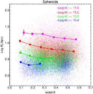
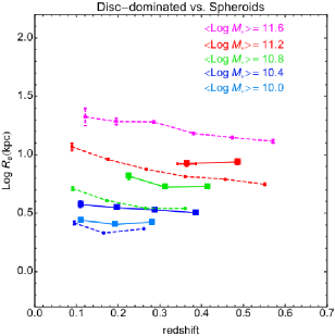
Figure 22: Size evolution with respect to z for spheroids (left) and disc-dominated galaxies (right) based on $r$ band data. In the left panel we show the spheroids average relation as full squares connected by solid lines against individual galaxy values colour coded according to their average mass in the mass bins. In the right panel disc-dominated values are given as squares connected by solid lines and spheroids are also reported as dotted lines as comparison. In each case mean for redshift are given and standard deviation of mean in size is given as the error bars as filled squares.

4.2.2 disc-dominated

The mass size relation of disc-dominated systems is shown in Fig. 20 as open symbols and compared with the ones of spheroids from Fig. 16. In all panels we show again the local relation, by M+13, but here represented as a shaded area which reproduces the larger spanning of their inferences, depending on the different selections made (LTG, $n<2.5$, blue samples, etc.). Our $z\sim 0$ results (top left) are again very well consistent with literature, and we can see a change in the overall slope at $\mbox{Log}\ M_{*}/M_{\odot}<9$ which is not reported in previous data. In all other redshift bins, we see that the size–mass data tend to tilt with respect to the local relation, around a fixed mass scale ($\mbox{Log}\ M_{*}/M_{\odot}\sim 10.5$).

In our sample, disc-dominated galaxies have always larger sizes than spheroids at masses $\mathrel{\hbox to0.0pt{\lower 3.5pt\hbox{\hskip 0.5pt$\sim$}\hss}\raise 0.5pt\hbox{$<$}}10^{11.0}M_{\odot}$, consistently with what is found in previous literature (e.g. vdW+14), while for higher masses we do not have a significant sample of disc-dominated galaxies (see also the $B_{z}$ values in Tab. 2 which are larger for the discs with respect to the passive galaxies at $\mbox{Log}\ M_{*}/M_{\odot}>10.8$) and we cannot exclude that spheroids might have larger sizes at that mass range, e.g., vdW+14. We expect to investigate more this issue with the next KiDS data release.

We finally see that disc-dominated galaxies do not show a clear trend with redshift as clearly seen for spheroids. In fact, in Fig. 20 the average relations at higher $z$ do not deviate significantly from the one at $z=0$ (shaded region) as observed in the case of spheroids.

As done for spheroids in Sect. 4.2.1, we have quantified the dependence on the redshift by fitting the $\mbox{$R_{\rm e}$}-M_{*}$ relations at the different redshifts and determining the intercept at different mass values. In this case we have used only the double power law formula (Eq. 5), since the data do not show any signature of the inversion of their trend at low masses. The results are shown in Fig. 21, for the highest mass bins for which the sample is complete at $z<0.5$. disc-dominated sizes show a flat trend with redshits (see also the best fit slopes in Tab. 2), much flatter that the spheroids. This is consistent with the results from vdW+14, also shown as thick shaded lines, using the same intercept approach.

In the same Fig. 21 (bottom panel) we have also estimated the trend with redshift of the size normalized to the local value and our results seem to have a trend which is spread in normalization but consistent with the ones obtained by, e.g., Trujillo et al. (2007). The new evidence from the KiDS sample is that galaxies in the lower mass bins have a trend which is similar to the one of the most massive bins (if we exclude the very massive one, which is incomplete at lower redshift), as also quantified in Tab. 2. Overall the disc-dominated systems show shallower trends than spheroids in all mass bins.

4.3 Spheroids and disc-dominated size evolution parametric fit

In this section we offer a complementary analysis of the size evolution by directly deriving the $\mbox{$R_{\rm e}$}-z$ relation in different mass bins. Being this inference independent of any fitting formula, it provides a more unbiased estimate of the actual dependence of the size from the redshift, once the the mass incompleteness in each redshift bin has been taken into account.

The results for the spheroids and disc-dominated galaxies are compared in Fig. 22, where we show the average $\mbox{$R_{\rm e}$}-z$ dependence in different mass bins, following the mass grouping and colour code adopted in the previous section. For the spheroids, we also show the individual values with the same colour code to better evaluate the spread of the relation. For disc-dominated galaxies we have omitted individual values because, being their relative normalization in the different mass bins smaller than the spheroids case (see average values, in the right panel, closer to each other wrt spheroids) and the scatter almost the same of the one of spheroids, it was too crowded to appreciate any difference among the different mass bins. We have performed also for these average estimates the $\mbox{$R_{\rm e}$}=B_{z}(1+z)^{\beta_{z}}$ fit, with best-fitting parameters being reported in Tab. 2.

Both the average values and the parametric fit show the same features discussed for the size-redshift obtained for the “indirect” relations in the previous Section. Namely, the spheroids show steeper decreasing trends with $z$ for mass bins $\mbox{Log}\ M_{*}~{}\hbox to0.0pt{$>$\hss}{\lower 4.30554pt\hbox{$\sim$}}10.5$ while they almost flatten out at lower masses. disc-dominated galaxies show shallower slopes (see Tab. 2) than spheroids and, at masses $\mbox{Log}\ M_{*}\mathrel{\hbox to0.0pt{\lower 3.5pt\hbox{\hskip 0.5pt$\sim$}\hss}\raise 0.5pt\hbox{$<$}}11.0$, they show larger sizes than the spheroids (see the comparison between spheroids and disc-dominated galaxies in Fig. 22, right panel). We will interpret these different variations of the size with $z$ in the next paragraph.

Looking at the average slopes in the Tab. 2, for the indirect fit we have a good agreement with vdW+14 (they have found a slope of -1.48 for their ETGs, we have an average of $-1.6\pm 0.3$), while our disc-dominated systems show possibly a shallower evolution as they find -0.75, while we have an average slope of $-0.5\pm 0.6$, but we are dominated here by the value of the high mass which is quite uncertain being based on two points. If we exclude that value, we obtain an average slope of $-0.7\pm 0.4$, hence consistent with the results from vdW+14. Overall these average quantities have a large scatter due primarily to the wide range of stellar masses covered. However, as shown in §4.2.1 and §4.2.2, the consistency with vdW+14 is generally very good in the mass bins. Similar average slopes are found for the direct fit in the same Table.

5 Discussion and Conclusions

The main result of this paper is that the two main classes of galaxies, spheroids and discs, show different relations between size and stellar mass and size and redshift, which are well consistent with previous literature (Shen et al. 2003, Baldry et al. 2012, van der Wel et al. 2014) but based on a sample which is much larger in the higher redshift bins. Our sample, complete in mass down to $\mbox{Log}\ M_{*}\mathrel{\hbox to0.0pt{\lower 3.5pt\hbox{\hskip 0.5pt$\sim$}\hss}\raise 0.5pt\hbox{$<$}}9.0$ at $z<0.2$ and down to $\mbox{Log}\ M_{*}~{}\hbox to0.0pt{$>$\hss}{\lower 4.30554pt\hbox{$\sim$}}10.0$ at higher$-z$, has allowed us to highlight some features that were not clearly assessed in previous datasets (at lower $z$, e.g. HB+09, S+03, M+13). First, a curvature in the $\mbox{$R_{\rm e}$}-M_{*}$, seems present at almost all $z$-bins for both spheroids and disc-dominated galaxies, but becomes less clear at $z>0.4$, mainly because of the mass incompleteness. The size–mass relation of disc-dominated galaxies also presents a knee in the relation at the very low masses ($\mbox{Log}\ M_{*}\mathrel{\hbox to0.0pt{\lower 3.5pt\hbox{\hskip 0.5pt$\sim$}\hss}\raise 0.5pt\hbox{$<$}}9.5$) at $z<0.1$, which was not reported in previous studies.

The results found for our spheroids and disc-dominated samples are consistent with the expectation of the galaxy growth from recent hydrodynamical simulations (Furlong et al. 2015) from the EAGLE set-up (Schaye et al. 2015), as demonstrated in Fig. 23. Overall, the predictions from simulations match our trends at all mass scales within $1\sigma$, although the match of the spheroids is slightly more discrepant with respect to the excellent agreement found for disc-dominated galaxies, especially for the higher mass values. However, the consistency of sizes predicted for spheroids in the EAGLE simulations and our estimates indirectly demonstrates the importance of feedback mechanisms to prevent the simulated systems to collapse too much. This is a well known effect of hydrodynamical simulations (e.g. Scannapieco & Athanassoula 2012) as a consequence of the so-called angular momentum catastrophe (Katz & Gunn 1991; Navarro & White 1994) consisting in a too large angular momentum transfer into the galaxy haloes which cannot retain the collapse of the cold gas into stars toward the galaxy center. The effect is todays balanced by the inclusion of feedback mechanisms in the centers, which balance the gas collapse (e.g. Governato et al. 2004; Sales et al. 2010; Hopkins et al. 2014; etc.), but whose recipes are still under refinement. In case an insufficient energy injection is accounted for in simulations, the predicted sizes result to be more compact for a given mass bin, as shown in the same Figure by the the predictions of the $\mbox{$R_{\rm e}$}-z$ for $\sim 10^{11}M_{\odot}$ spheroids from Oser et al. (2012) (note that they do not provide explicitly disc-dominated predictions) with a modified version of the parallel TreeSPH code GADGET-2 (Springel 2005) and no AGN feedback. The predicted sizes, in this case, turn out to be more than $1\sigma$ smaller the one derived in our analysis at all redshift.

The remarkable result that emerges from this comparison is that the observed sizes are naturally explained in the context of the galaxy assembly described in the cosmological simulations. In particular, the size growth is interpreted in Furlong et al. (2015) as the consequence of the accreted mass fraction since $z=2$. The more stellar mass is accreted from sources other than the main progenitor at a given time the more the final size of a galaxy is found to increase. This does not take into account the type of mergers that contribute to the size growth, but clearly establish that size growth and accreted mass fraction are inherently related (see their Fig. 5).

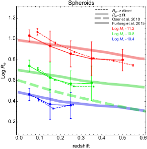
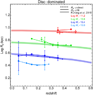
Figure 23: Comparison with hydrodynamical simulations. Left panel: spheroids size–redshift relation is compared with the EAGLE simulations from Furlong et al. (2015) and with a modified version of GADGET-2 from Oser et al. (2012). The data points show the results obtained in Sects. 4.2.1 (solid lines) and 4.2.2 (dashed lines) in different mass bins as in the legends. Right panel: disc-dominated size–redshift relation with symbols as in the left panel but with the results from the average-size mass from Sect. 4.2.2 (solid lines).

To conclude, in this paper we have demonstrated the large potential of the KiDS dataset for the structural parameter analysis of galaxies at least up to $z=0.6$. We have analyzed a sample of $\sim 380,000$ galaxies with signal-to-noise ratio large enough ($\mbox{$S/N$}_{r}>50$) to derive accurate structural parameters. Based on mock galaxy images and performing an external comparison, we have demonstrated that our estimates are robust. We have used in particular the size and stellar masses to investigate the evolution of the size-mass relation up to $z\sim 0.6$ and compared the results with hydrodynamical simulations for galaxy assembly. The main results of our analysis can be summarized as follows:

• The size–mass–redshift relation show a very good agreement with the size–mass and the size–redshift correlations obtained either in local analyses (e.g. Shen et al. 2003, Baldry et al. 2012, Mosleh et al. 2013) or at higher-$z$ (e.g. Trujillo et al. 2007, van der Wel et al. 2014). The size–mass relation of spheroids shows a clear evolution of the average quantities with redshift which we have interpreted as a consequence of the size decreases with increasing redshift at masses larger than $\mbox{Log}\ M_{*}/M_{\odot}\sim 10.5$, while the evolution of the sizes for the disc-dominated galaxies is very weak, which produces no appreciable evolution of their size–mass relations.

• We have derived the $R_{\rm e}$ vs. $z$ evolution using two approaches: 1) by fitting the size–mass relation at different redshift bins and then estimating the $\mbox{$R_{\rm e}$}-z$ evolution along different mass intercepts (see Sect. 4.2.1 and Sect. 4.2.2) and 2) by direct fitting the measured $R_{\rm e}$ vs. $z$ in different mass bins. The results of the two methods consistently show a substantial evolution of sizes with redshift, with spheroids having a steeper decrease of their sizes with increasing redshifts with respect to disc-dominated galaxies. The normalization and slope of the the $R_{\rm e}$ vs. $z$, parameterized using the standard $\mbox{$R_{\rm e}$}/kpc\propto(1+z)^{\beta_{z}}$ relation (see Tab. 2), are consistent with a recent analysis using accurate HST size measurements with single Sérsic profiles (van der Wel et al. 2014).

• We have compared the data with suites of recent hydrodynamical simulations of galaxy assembly with a full treatment of galaxy feedback (including supernovae and AGN feedback, Furlong et al. 2015), showing that also in this case our results are well matched by simulations and alway consistent with $1\sigma$ scatter of our observationally inferred $\mbox{$R_{\rm e}$}-z$ relations in different mass bins for both the spheroids and disc-dominated systems. We have also checked that simulations with no AGN feedback (e.g. from Oser et al. 2012) show a large discrepancy, showing that an insufficient feedback recipe produces a tension with data, due to the too compact sizes in simulated galaxies.

The large sample expected from KiDS and the image quality will allow us to obtain unprecedented details in the evolution of the galaxy size and mass over the cosmic time, which can be compared with expectations from simulations. We expect to expand considerably the analysis presented in this paper with the next KiDS data releases, both in terms of size and depth of the sample, as we will gather statistics toward higher redshift to confirm our trends.

Appendix A Effect of the errors on the $\boldsymbol{$\mbox{$R_{\rm e}$}-z$}$ relations

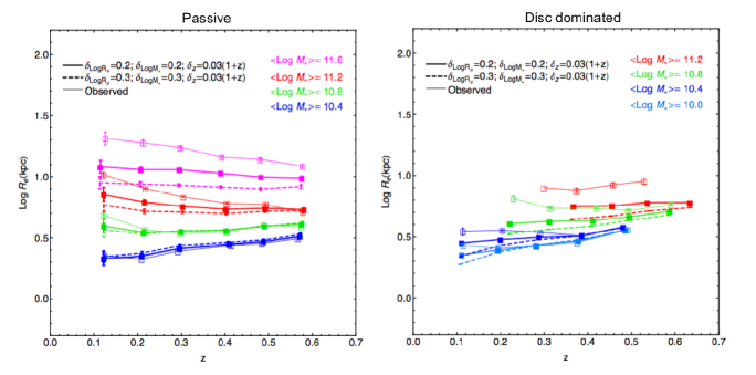
Figure 24: Effect of the errors on the $R_{\rm e}$-$z$ correlation as derived in Fig. 22. Left: average trend for the spheroid sample obtained by resampling the original sample parameters by adding a shift from a Gaussian distribution using average errors (solid line) and maximum errors (dashed lines) as in the legends. The observed trend is also shown as comparison (tiny solid line). Right: the same as in the left panel for the disc dominated galaxies.

We want to check the effect of the uncertainties on the different quantities entering into the size-redshift trends discussed in Sects. 4.2.1 and 4.2.2. The trend found can indeed be affected by the intrinsic scatter of the mass, effective radius estimate and photometric redshift. In principle, the covariance among the individual errors might spuriously generate a correlation from the observed quantities. On the other way around, the observed trend can be even shallower than the intrinsic one for the scatter due to the different quantities that move objects from one bin to another, hence diluting the real trends. In order to check for the presence of these effects, and evaluate in which direction the correlations that we have derived in Sects. 4.2.1 and 4.2.2 and reported in Tab. 2 can be biased by the intrinsic scatter of the individual parameters, we have performed a series of bootstrap experiments to obtain random resamplings of our datasets. We have perturbed galaxy mass, $R_{\rm e}$ and $z_{\rm phot}$ by randomly adding a offset extracted from a Gaussian distribution having zero mean and a constant standard deviation equal to the average error of the different quantities (namely $\sigma_{\mbox{Log}\ M_{*}}$, $\sigma_{\mbox{$R_{\rm e}$}}$, $\sigma_{\mbox{$z_{\rm phot}$}}$ for the mass, size and $z_{\rm phot}$ respectively), hence resampling the same observed relations, but adding the effect of random errors on the individual parameters.

In Sect. 2.3 we have mentioned that average errors on masses are of the order of 0.2 dex (maximum errors reaching 0.3 dex), while the relative errors on $R_{\rm e}$ are of the order of 15 per cent (20 per cent maximum, see e.g. Figs. 12, 13, and 14), while the scatter for the $z_{\rm phot}$ has been reported to be of the order of $0.03(1+z_{\rm spec})$ (see Sect. 2.2). We have re-extracted the catalog values 100 times and obtained, at every extraction, a correlation like Fig. 22, which we have finally averaged to obtain the average trend in each mass bin.

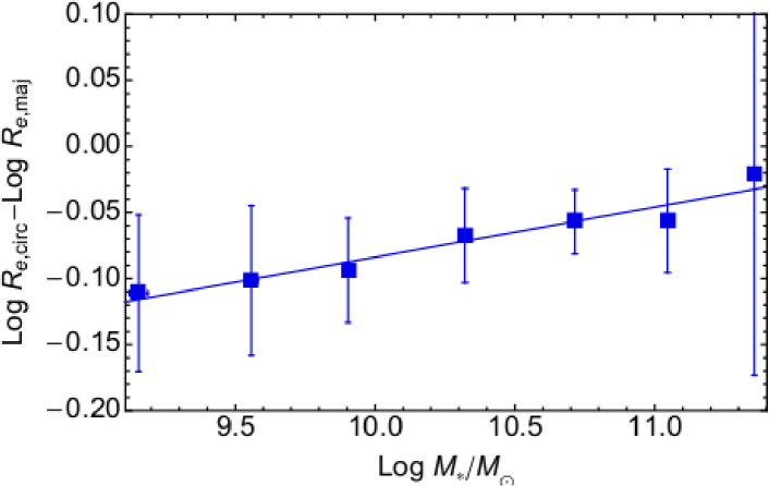
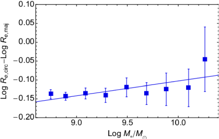
Figure 25: Differences between the (log) circularized and major axis effective radii obtained with 2DPHOT for KiDS spheroids (top) and disc dominated (bottom) in $r$-band as a function of the stellar mass in the lowest redshift bin as in Fig. 16. Mean differences and standard deviations are shown as data points with error bars, together with a linear fit to the data. This shows the statistical correction one should apply to the size-mass relation in the case of major axis size estimates (as for B+12 and K+12).

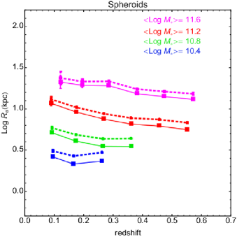
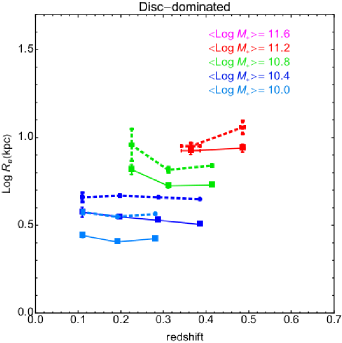
Figure 26: Size-redshift correlation for the spheroids (left) and disc dominated galaxies (right) using the circularized (solid line) or the major axis effective radii (dashed line).

We have also checked that the quantities that are affecting more the trend is the mass as the scattered quantities move galaxies from the central mass bins to the contiguous (small and larger mass) ones, hence making all relations to converge toward the ones of the intermediate bins, as shown from the case of maximum errors.

In Fig. 24 we show the “bootstrap” results for spheroids and disc-dominated galaxies obtained both for the average errors (solid lines) and for the maximum errors (dashed lines). We can clearly see that for the spheroids, the larger the errors assumed the flatter is the final trend obtained. This demonstrate that the effect of the uncertainties on the quantities is statistically to reduce the steepness of the observed trends (tiny lines in Fig. 24) rather then to introduce a spurious slope. The same effect is also seen for the disc-dominated galaxies although, for the lower mass bin, we see that errors produce a steepening of the correlation in the lower redshift bins.

Overall, this test demonstrates that the trends discussed in Tab. 2 are real and possibly shallower than the ones that we had measured if we could reduce the uncertainties on the observed quantities. The only exception is for low-mass disc-dominated systems (i.e. $\mbox{Log}\ M_{*}/M_{\odot}\mathrel{\hbox to0.0pt{\lower 3.5pt\hbox{\hskip 0.5pt$\sim$}\hss}\raise 0.5pt\hbox{$<$}}10.2$), that at lower redshift ($z<0.2$) might have a steeper trend with respect to the almost flat trend observed in Fig. 22.

As discussed above, the major source of uncertainties in the derived trends is the one on the mass, which we plan to reduce in the future by adding NearInfraRed (NIR) bands in our SED estimates.

Appendix B Effect of the size definition: circularized vs. major axis effective radius

In this section we want to statistical assess the effect of the size definition on the size mass relations discussed in §4. We have seen that different analyses have made different choices on the effective radius to use for their relations, i.e. by using the simple major axis radius ($R_{m}$, which does not take into account the observed flattening of the galaxy) or the circularized one, defined as $\mbox{$R_{\rm e}$}=(b/a)^{1/2}R_{m}$ (as done in §3.1). Since the axis ratio changes with the luminosity and mass of galaxies, the ratio between the $R_{\rm e}$ and $R_{m}$, which is exactly $f=\sqrt{b/a}$, also changes with these parameters and hence one should measure a tilt of the size-mass relation depending on whether this is based on the use of $R_{\rm e}$ or $R_{m}$. We can quantify how the ratio of the two quantities $f=\sqrt{b/a}$ changes with stellar mass for the KiDS spheroids and disc dominated galaxies by looking at the difference of the logarithm of these two radii in Fig. 25.

In the plot we see that for spheroids $\mbox{$R_{\rm e}$}/R_{m}$ is almost equal to one for the more massive galaxies (which are dominated by early-type rounder systems) and then decreases for lower masses consistently with the known anti-correlation between the flattening and the mass, i.e. the axis ratio tends to increase for lower mass systems. This is more marked for disc dominated systems which are intrinsically flatter at almost all masses. If on one hand, we can use the correlation shown in Fig. 25 to convert the correlations found in §4 for the circularized radii into the same correlations for the major axis sizes, on the other hand we can use the same correlation to rescale the literature results based on major axis sizes to the circularized size they should have if they statistically have the same flattening variation with mass as the KiDS sample. We note that, in practice, the operation of correcting the circularized radii of the KiDS data to match the major axis definition of other analysis (e.g. B+12 and K+12) would bring to the same conclusion if the major axis data would be converted into the circularized ones using the inverse ratio $1/f$, but with a different normalization, which is the approach we used for Fig. 16, when comparing different results from literature.

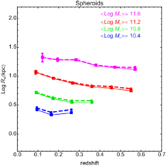
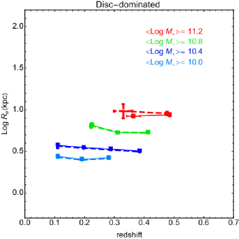
Figure 27: Size–redshift correlation for the spheroids (left) and disc dominated galaxies (right) using $n=2.5$ (solid line, see also Fig. 22) or $n=3.5$ (dashed line).

In order to better quantify the effect of the size definition on our results, we compare the Size vs. $z$ relations of the spheroids and disc-dominated systems in Fig. 26, obtained both for the $R_{\rm e}$and $R_{m}$. The major effect is seen in the normalization of the relations, being the $R_{m}$ generally larger than the $R_{\rm e}$ and it is more evident for disc-dominated systems which are intrinsically more flattened. Also, there is a tendency to show a larger difference toward higher-z, being generally all systems less round going back in time in their evolution. Overall, the $R_{m}$ vs. redshift does not seem to drive to different conclusions of the one discussed for the $R_{\rm e}$, with spheroids showing a gain a significant growth toward low-z and the disc-dominated systems almost no evolutions at all all mass scales.

Appendix C Effect of the Sérsic index systematics

In §3.4.2 we have found a systematic offset of the $n$-index estimated with 2DPHOT with respect to the ones by GALFIT in the sample common to the SDSS analysed in K+12. We have discussed that it is not possible at the moment to assess which of the two set of inferences is unbiased. Despite our test on mock galaxies in §3.3.2 shows no bias in the 2DPHOT estimates, we want to quantify which would be the effect of of a biased the spheroids/discs splitting of our sample on the final size evolution, if our Sérsic index are systematic overestimate of ground truth, assuming these latter given by the ones from GALFIT on GAMA galaxies. If this is the case, then our criterion of $n>2.5$ to select spheroids should have possibly including a large fraction of actual discs. We recall here that the galaxy classification we have adopted is based on both the Sérsic index cut and SED classes as discussed in §2.3, and the former only partially plays a role.

To proceed with this test we decided to compare the results on the size-redshift relation obtained with $n=2.5$ as discriminant for spheroids/discs with the same relation obtained for $n=3.5$, which is a more conservative value in case the 2DPHOT estimates correspond to intrinsically smaller $n$-indexes. This is shown in Fig. 27, where we can see that the change of the correlations for the spheroid and disc-dominated galaxies are almost unchanged. This shows that the combination of the $n$-index and the SED class basically prevents significant misclassifications which might be expected in the case only $n$-index would be used.

Appendix D Effect of wavelength on the $R_{\rm e}$

Galaxies have color gradients, which means that, on average, their optical $R_{\rm e}$ can change as a function of the band in which they are observed. E.g. spheroids have negative gradients (they are redder in their center and bluer in their outskirts) which implies that they are larger in bluer bands (see e.g., Sparks & Jorgensen 1993; Hyde & Bernardi 2009; La Barbera & de Carvalho 2009; La Barbera et al. 2010a; Roche et al. 2010; Tortora et al. 2010; Tortora et al. 2018c; Vulcani et al. 2014; Beifiori et al. 2014).

Going to higher redshifts, the blue part of galaxy SEDs are redshifted into redder bands, hence the $r$-band which we have used as reference band for our analysis, covers different rest frame wavelengths in different galaxies, depending on each galaxy redshift. If the colour gradients persist at these epochs, this implies that the observed frame $r$-band of a high-$z$ galaxy, which corresponds to a $g$-band rest frame, is intrinsically larger than the $r$-band of a lower-$z$, which is closer to the $r$-band rest frame itself (see Vulcani et al. 2014). E.g., the mean wavelengths of OmegaCAM filters are $\lambda_{g,r,i}=\{4770,6231,7625\}$ Å, i.e. a galaxy at $z=0$ observed in $g$-band at $\lambda_{g}=4770$Å is redshifted to $\lambda_{r}=6287$Å for $z=0.32$, and to the lower limit of the $r$-band wavelength range $\lambda_{r,min}\sim 5200$Å for $z\sim 0.1$ (see Fig. 28).

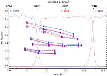
Figure 28: Size–redshift relation for the spheroids (solid lines) in the mass bins $\mbox{Log}\ M_{*}/M_{\odot}=$10.4, 10.8, 11.2 and disc dominated galaxies in the mass bins $\mbox{Log}\ M_{*}/M_{\odot}=$10.0, 10.4, 10.8 (dashed lines) in $g$ (blue), $r$ (red) and $i$ (purple) bands.

The top axis reports the wavelength of the $g$-band central $\lambda_{g}=4770$Å redshifted according to the corresponding $z$ on the bottom axis. The filter response in arbitrary units are shown with the wavelength consistent with the top axis. See text for more details.

This implies that if we use $r$-band as a reference for galaxies at lower (e.g. $z\mathrel{\hbox to0.0pt{\lower 3.5pt\hbox{\hskip 0.5pt$\sim$}\hss}\raise 0.5pt\hbox{$<$}}0.15$) and higher redshift (e.g. $z~{}\hbox to0.0pt{$>$\hss}{\lower 4.30554pt\hbox{$\sim$}}0.15$), in case the ones at higher-$z$ have negative colour gradients, these might look larger than the ones at lower-$z$ because their emission in $r$-band is dominated by the rest-frame $g$-band. The opposite will happen for galaxies at higher-$z$ with positive gradient.

To quantify this effect we could proceed in two ways. First, we can check whether there is an observed difference between the average $R_{\rm e}$ estimated in bins of redshift and mass in the different bands. Second, we could compute the rest frame $R_{\rm e}$ at some reference wavelength by linearly interpolating the $R_{\rm e}$ values obtained in different bands and estimate the evolution with redshift of this latter. We will show that the second approach is not convenient to apply at this stage of the project since we are lacking of completeness and sample size, to have robust inferences. We limit here to demonstrate that the adoption of the deeper $r$-band is not expected to affect the main results of our paper.

Looking at the $\mbox{$R_{\rm e}$}-z$ in the other bands, it is important to check the mass dependence because color gradients have been observed to change with mass (La Barbera & de Carvalho 2009; La Barbera et al. 2010a; Tortora et al. 2010; Tortora et al. 2018c). In order to do that we needed to use a mass complete sample of galaxies for which we have measurements of the $R_{\rm e}$ in the $gri$ bands simultaneously (we have excluded the $u$-band since this would have reduced the sample too much, see below) and selected also in this case the ones with highest $S/N$ $(>50)$ and best $\chi^{2}~{}(<1.3)$. Since the depth and completeness mass in the $g$- and $i$-band are lower than the $r$-band because of the survey strategy, the final sample of galaxies available for this test is almost one third of the one found for $r$-band (see §4.1), i.e. $\sim 70$k galaxies.

In Fig. 28 (left) we show the average $\mbox{$R_{\rm e}$}-z$ of the selected sample of galaxies in $gri$-bands for the spheroids (solid lines) and disc-dominated (dashed lines). In particular, we show the relations obtained for different mass bins (bottom lines with smaller $R_{\rm e}$ to the top), which are $\mbox{Log}\ M_{*}/M_{\odot}=$10.4, 10.8, 11.2 for spheroids and $\mbox{Log}\ M_{*}/M_{\odot}=$10.0, 10.4, 10.8 for disc-dominated galaxies. In the same figure we show on the top axis the wavelength of the $g$-band central $\lambda_{g}=4770$Å redshifted according to the corresponding $z$ on the bottom axis. We also overplot the filter response in arbitrary units with the wavelength distributed according to the top axis. This allows us to visualize how the $g$-band rest frame is shifted into other bands at any redshift, and compare this with the $R_{\rm e}$ inferences in the different bands. We can see that the adoption of the $r$-band as a reference filter for our analysis is motivated by the fact that this covers the largest part of the redshift window of our sample (i.e. $z=0.1$ to $0.5$). If one would fairly compare the galaxy sizes in the same rest frame wavelength range, than the $g$-band estimates would work approximately until $z\sim 0.15$ and the $r$-band between $z\sim 0.15$ and $z\sim 0.45$, while $i$-band should be used at $z~{}\hbox to0.0pt{$>$\hss}{\lower 4.30554pt\hbox{$\sim$}}0.45$.

Overall, we see that the disc-dominated galaxies show almost no differences in the $R_{\rm e}$ estimates in all bands and for the lower mass bin, they look almost undistinguishable. This suggests that discs have almost no colour gradients or possibly mild negative one. This latter is more evident for the larger mass bin at low-z, which goes along the direction of previous finding in local samples (e.g., Tortora et al. 2010). Spheroids show negative gradients at almost all mass (and increasing with it) and redshift, except possibly for the $g-r$ of the most massive systems at low-$z$, where the $g$- and $r$-band estimates almost coincide. On the other hand the $r$- and $i$-band average estimates are almost identical at all masses and redshift except for the latter case. The spheroids negative gradients are also larger for more massive systems.

The discussion on the trends of the colour gradients is beyond the scopes of this paper, and there will be forthcoming analysis dedicated to that, here we are interested on the effect of these gradients on the main conclusions of our paper. As anticipated, the presence of negative gradients would imply that, while the measurement of the $r$-band at $0.15\mathrel{\hbox to0.0pt{\lower 3.5pt\hbox{\hskip 0.5pt$\sim$}\hss}\raise 0.5pt\hbox{$<$}}z\mathrel{\hbox to0.0pt{\lower 3.5pt\hbox{\hskip 0.5pt$\sim$}\hss}\raise 0.5pt\hbox{$<$}}0.45$ are a good representation of the rest frame $g$-band, at lower $z$ it is the $g$-band $R_{\rm e}$ the one to use. But these latter are systematically larger than the ones from $r$-band and hence the slope that we would measure should be steeper that the one obtained using the $r$-band at all redshift. Note that even if the $i$-band would represent the ideal band to cover the $g$-band rest frame at $z>0.45$, being $r$ and $i$-band estimates almost identical, we do not expect that the use of $r$-band has caused any effect.

In this perspective the only big change we could expect by using proper rest frame sizes would be a steepening of the correlation with $z$ toward the lower redshift. Since the current sample of galaxies analysed in the three $gri$ bands is limited in number, mass and redshift (see Fig. 28), we reserve this analysis to next datasets from the subsequent data releases. E.g., we expect to collect up to 500k galaxies with $gri$ sizes in a larger photo-z range (using the updated estimates from Bilicki et al. 2017) with the upcoming KiDS data release 4 based on 900 deg² of the survey.

References

- Ahn et al. (2012) Ahn C. P., et al., 2012, ApJS, 203, 21
- Arnouts et al. (1999) Arnouts S., Cristiani S., Moscardini L., Matarrese S., Lucchin F., Fontana A., Giallongo E., 1999, MNRAS, 310, 540
- Arnouts et al. (2001) Arnouts S., et al., 2001, A&A, 379, 740
- Baldry et al. (2012) Baldry I. K., et al., 2012, MNRAS, 421, 621
- Beifiori et al. (2014) Beifiori A., et al., 2014, preprint (arXiv:1405.1431)
- Bernardi et al. (2003) Bernardi M., et al., 2003, AJ, 125, 1882
- Bertin & Arnouts (1996) Bertin E., Arnouts S., 1996, A&AS, 117, 393
- Bezanson et al. (2009) Bezanson R., van Dokkum P. G., Tal T., Marchesini D., Kriek M., Franx M., Coppi P., 2009, ApJ, 697, 1290
- Bilicki et al. (2017) Bilicki M., et al., 2017, ArXiv:1709.04205
- Bower et al. (1992) Bower R. G., Lucey J. R., Ellis R. S., 1992, MNRAS, 254, 601
- Brescia et al. (2013) Brescia M., Cavuoti S., D’Abrusco R., Longo G., Mercurio A., 2013, ApJ, 772, 140
- Brescia et al. (2014) Brescia M., Cavuoti S., Longo G., De Stefano V., 2014, A&A, 568, A126
- Bruzual & Charlot (2003) Bruzual G., Charlot S., 2003, MNRAS, 344, 1000
- Capaccioli & Schipani (2011) Capaccioli M., Schipani P., 2011, The Messenger, 146, 2
- Capaccioli et al. (1992) Capaccioli M., Caon N., D’Onofrio M., 1992, MNRAS, 259, 323
- Capak et al. (2004) Capak P., et al., 2004, AJ, 127, 180
- Cappellari et al. (2012) Cappellari M., et al., 2012, Nature, 484, 485
- Cardone et al. (2011) Cardone V. F., Del Popolo A., Tortora C., Napolitano N. R., 2011, MNRAS, 416, 1822
- Cassata et al. (2010) Cassata P., et al., 2010, ApJ, 714, L79
- Cavuoti et al. (2015a) Cavuoti S., Brescia M., De Stefano V., Longo G., 2015a, Experimental Astronomy, 39, 45
- Cavuoti et al. (2015b) Cavuoti S., et al., 2015b, MNRAS, 452, 3100
- Cavuoti et al. (2017) Cavuoti S., et al., 2017, MNRAS, 466, 2039
- Chabrier (2001) Chabrier G., 2001, ApJ, 554, 1274
- Coleman et al. (1980) Coleman G. D., Wu C.-C., Weedman D. W., 1980, ApJS, 43, 393
- Colless et al. (2001) Colless M., et al., 2001, MNRAS, 328, 1039
- Conroy & van Dokkum (2012) Conroy C., van Dokkum P. G., 2012, ApJ, 760, 71
- Courteau et al. (2007) Courteau S., Dutton A. A., van den Bosch F. C., MacArthur L. A., Dekel A., McIntosh D. H., Dale D. A., 2007, ApJ, 671, 203
- D’Onofrio et al. (1997) D’Onofrio M., Capaccioli M., Zaggia S. R., Caon N., 1997, MNRAS, 289, 847
- Daddi et al. (2005) Daddi E., et al., 2005, ApJ, 626, 680
- Damjanov et al. (2015) Damjanov I., Geller M. J., Zahid H. J., Hwang H. S., 2015, ApJ, 806, 158
- Davis et al. (2003) Davis M., et al., 2003, in Guhathakurta P., ed., Proc. SPIEVol. 4834, Discoveries and Research Prospects from 6- to 10-Meter-Class Telescopes II. pp 161–172 (arXiv:astro-ph/0209419), doi:10.1117/12.457897
- Dressler et al. (1987) Dressler A., Lynden-Bell D., Burstein D., Davies R. L., Faber S. M., Terlevich R., Wegner G., 1987, ApJ, 313, 42
- Driver et al. (2011) Driver S. P., et al., 2011, MNRAS, 413, 971
- Dutton et al. (2007) Dutton A. A., van den Bosch F. C., Dekel A., Courteau S., 2007, ApJ, 654, 27
- Faber & Jackson (1976) Faber S. M., Jackson R. E., 1976, ApJ, 204, 668
- Fan et al. (2008) Fan L., Lapi A., De Zotti G., Danese L., 2008, ApJ, 689, L101
- Ferrarese & Merritt (2000) Ferrarese L., Merritt D., 2000, ApJ, 539, L9
- Franx et al. (2008) Franx M., van Dokkum P. G., Förster Schreiber N. M., Wuyts S., Labbé I., Toft S., 2008, ApJ, 688, 770
- Furlong et al. (2015) Furlong M., et al., 2015, MNRAS, 450, 4486
- Gebhardt et al. (2000) Gebhardt K., et al., 2000, ApJ, 539, L13
- Governato et al. (2004) Governato F., et al., 2004, ApJ, 607, 688
- Guo & White (2008) Guo Q., White S. D. M., 2008, MNRAS, 384, 2
- Guzman et al. (1992) Guzman R., Lucey J. R., Carter D., Terlevich R. J., 1992, MNRAS, 257, 187
- Hildebrandt et al. (2017) Hildebrandt H., et al., 2017, MNRAS, 465, 1454
- Hilz et al. (2013) Hilz M., Naab T., Ostriker J. P., 2013, MNRAS, 429, 2924
- Hopkins et al. (2009) Hopkins P. F., Lauer T. R., Cox T. J., Hernquist L., Kormendy J., 2009, ApJS, 181, 486
- Hopkins et al. (2014) Hopkins P. F., Kereš D., Oñorbe J., Faucher-Giguère C.-A., Quataert E., Murray N., Bullock J. S., 2014, MNRAS, 445, 581
- Huertas-Company et al. (2013) Huertas-Company M., et al., 2013, MNRAS, 428, 1715
- Hyde & Bernardi (2009) Hyde J. B., Bernardi M., 2009, MNRAS, 394, 1978
- Ilbert et al. (2006) Ilbert O., et al., 2006, A&A, 457, 841
- Iodice et al. (2016) Iodice E., et al., 2016, ApJ, 820, 42
- Kashikawa et al. (2004) Kashikawa N., et al., 2004, PASJ, 56, 1011
- Katz & Gunn (1991) Katz N., Gunn J. E., 1991, ApJ, 377, 365
- Kauffmann (1996) Kauffmann G., 1996, MNRAS, 281, 487
- Kauffmann et al. (2003) Kauffmann G., et al., 2003, MNRAS, 341, 54
- Kelvin et al. (2012) Kelvin L. S., et al., 2012, MNRAS, 421, 1007
- Kelvin et al. (2014) Kelvin L. S., et al., 2014, MNRAS, 444, 1647
- Kinney et al. (1996) Kinney A. L., Calzetti D., Bohlin R. C., McQuade K., Storchi-Bergmann T., Schmitt H. R., 1996, ApJ, 467, 38
- Koekemoer et al. (2011) Koekemoer A. M., et al., 2011, ApJS, 197, 36
- Komatsu et al. (2011) Komatsu E., et al., 2011, ApJS, 192, 18
- Kormendy (1977) Kormendy J., 1977, ApJ, 218, 333
- Kormendy et al. (2009) Kormendy J., Fisher D. B., Cornell M. E., Bender R., 2009, ApJS, 182, 216
- Kuijken et al. (2015) Kuijken K., et al., 2015, MNRAS, 454, 3500
- La Barbera & de Carvalho (2009) La Barbera F., de Carvalho R. R., 2009, ApJ, 699, L76
- La Barbera et al. (2002) La Barbera F., Busarello G., Merluzzi P., Massarotti M., Capaccioli M., 2002, ApJ, 571, 790
- La Barbera et al. (2008) La Barbera F., de Carvalho R. R., Kohl-Moreira J. L., Gal R. R., Soares-Santos M., Capaccioli M., Santos R., Sant’anna N., 2008, PASP, 120, 681
- La Barbera et al. (2010a) La Barbera F., De Carvalho R. R., De La Rosa I. G., Gal R. R., Swindle R., Lopes P. A. A., 2010a, AJ, 140, 1528
- La Barbera et al. (2010b) La Barbera F., de Carvalho R. R., de La Rosa I. G., Lopes P. A. A., Kohl-Moreira J. L., Capelato H. V., 2010b, MNRAS, 408, 1313
- La Barbera et al. (2011) La Barbera F., Ferreras I., de Carvalho R. R., Lopes P. A. A., Pasquali A., de la Rosa I. G., De Lucia G., 2011, ApJ, 740, L41
- La Barbera et al. (2013) La Barbera F., Ferreras I., Vazdekis A., de la Rosa I. G., de Carvalho R. R., Trevisan M., Falcón-Barroso J., Ricciardelli E., 2013, MNRAS, 433, 3017
- Lange et al. (2015) Lange R., et al., 2015, MNRAS, 447, 2603
- Lelli et al. (2016) Lelli F., McGaugh S. S., Schombert J. M., 2016, ApJ, 816, L14
- Magorrian et al. (1998) Magorrian J., et al., 1998, AJ, 115, 2285
- McCracken et al. (2003) McCracken H. J., et al., 2003, A&A, 410, 17
- Mo et al. (1998) Mo H. J., Mao S., White S. D. M., 1998, MNRAS, 295, 319
- Mosleh et al. (2013) Mosleh M., Williams R. J., Franx M., 2013, ApJ, 777, 117
- Moster et al. (2010) Moster B. P., Somerville R. S., Maulbetsch C., van den Bosch F. C., Macciò A. V., Naab T., Oser L., 2010, ApJ, 710, 903
- Muzzin et al. (2009) Muzzin A., van Dokkum P., Franx M., Marchesini D., Kriek M., Labbé I., 2009, ApJ, 706, L188
- Naab et al. (2009) Naab T., Johansson P. H., Ostriker J. P., 2009, ApJ, 699, L178
- Napolitano et al. (2016) Napolitano N. R., et al., 2016, The Universe of Digital Sky Surveys, 42, 129
- Navarro & White (1994) Navarro J. F., White S. D. M., 1994, MNRAS, 267, 401
- Oser et al. (2012) Oser L., Naab T., Ostriker J. P., Johansson P. H., 2012, ApJ, 744, 63
- Peng et al. (2002) Peng C. Y., Ho L. C., Impey C. D., Rix H.-W., 2002, AJ, 124, 266
- Petrillo et al. (2017) Petrillo C. E., et al., 2017, MNRAS, 472, 1129
- Radovich et al. (2017) Radovich M., et al., 2017, A&A, 598, A107
- Ravindranath et al. (2002) Ravindranath S., et al., 2002, in American Astronomical Society Meeting Abstracts. p. 1099
- Roche et al. (2010) Roche N., Bernardi M., Hyde J., 2010, MNRAS, 407, 1231
- Rykoff et al. (2015) Rykoff E. S., Rozo E., Keisler R., 2015, preprint (arXiv:1509.00870)
- Saglia et al. (2010) Saglia R. P., et al., 2010, A&A, 524, A6
- Sales et al. (2010) Sales L. V., Navarro J. F., Schaye J., Dalla Vecchia C., Springel V., Booth C. M., 2010, MNRAS, 409, 1541
- Scannapieco & Athanassoula (2012) Scannapieco C., Athanassoula E., 2012, MNRAS, 425, L10
- Schaye et al. (2015) Schaye J., et al., 2015, MNRAS, 446, 521
- Schlafly & Finkbeiner (2011) Schlafly E. F., Finkbeiner D. P., 2011, ApJ, 737, 103
- Shen et al. (2003) Shen S., Mo H. J., White S. D. M., Blanton M. R., Kauffmann G., Voges W., Brinkmann J., Csabai I., 2003, MNRAS, 343, 978
- Sparks & Jorgensen (1993) Sparks W. B., Jorgensen I., 1993, AJ, 105, 1753
- Spiniello et al. (2018) Spiniello C., et al., 2018, preprint (arXiv:1805.12436)
- Springel (2005) Springel V., 2005, MNRAS, 364, 1105
- Strateva et al. (2001) Strateva I., et al., 2001, AJ, 122, 1861
- Szomoru et al. (2010) Szomoru D., et al., 2010, ApJ, 714, L244
- Tortora et al. (2009) Tortora C., Napolitano N. R., Romanowsky A. J., Capaccioli M., Covone G., 2009, MNRAS, 396, 1132
- Tortora et al. (2010) Tortora C., Napolitano N. R., Cardone V. F., Capaccioli M., Jetzer P., Molinaro R., 2010, MNRAS, 407, 144
- Tortora et al. (2012) Tortora C., La Barbera F., Napolitano N. R., de Carvalho R. R., Romanowsky A. J., 2012, MNRAS, 425, 577
- Tortora et al. (2013) Tortora C., Romanowsky A. J., Napolitano N. R., 2013, ApJ, 765, 8
- Tortora et al. (2014a) Tortora C., Romanowsky A. J., Cardone V. F., Napolitano N. R., Jetzer P., 2014a, MNRAS, 438, L46
- Tortora et al. (2014b) Tortora C., La Barbera F., Napolitano N. R., Romanowsky A. J., Ferreras I., de Carvalho R. R., 2014b, MNRAS, 445, 115
- Tortora et al. (2014c) Tortora C., Napolitano N. R., Saglia R. P., Romanowsky A. J., Covone G., Capaccioli M., 2014c, MNRAS, 445, 162
- Tortora et al. (2016) Tortora C., et al., 2016, MNRAS, 457, 2845
- Tortora et al. (2018a) Tortora C., et al., 2018a, preprint (arXiv:1806.01307)
- Tortora et al. (2018b) Tortora C., Napolitano N. R., Roy N., Radovich M., Getman F., Koopmans L. V. E., Verdoes Kleijn G. A., Kuijken K. H., 2018b, MNRAS, 473, 969
- Tortora et al. (2018c) Tortora C., Napolitano N. R., Roy N., Radovich M., Getman F., Koopmans L. V. E., Verdoes Kleijn G. A., Kuijken K. H., 2018c, MNRAS, 473, 969
- Tremaine et al. (2002) Tremaine S., et al., 2002, ApJ, 574, 740
- Treu et al. (2010) Treu T., Auger M. W., Koopmans L. V. E., Gavazzi R., Marshall P. J., Bolton A. S., 2010, ApJ, 709, 1195
- Trujillo et al. (2006) Trujillo I., et al., 2006, ApJ, 650, 18
- Trujillo et al. (2007) Trujillo I., Conselice C. J., Bundy K., Cooper M. C., Eisenhardt P., Ellis R. S., 2007, MNRAS, 382, 109
- Trujillo et al. (2011) Trujillo I., Ferreras I., de La Rosa I. G., 2011, MNRAS, 415, 3903
- Trujillo et al. (2012) Trujillo I., Carrasco E. R., Ferré-Mateu A., 2012, ApJ, 751, 45
- Tully & Fisher (1977) Tully R. B., Fisher J. R., 1977, A&A, 54, 661
- Vulcani et al. (2014) Vulcani B., et al., 2014, MNRAS, 441, 1340
- Yasuda et al. (2001) Yasuda N., et al., 2001, AJ, 122, 1104
- York et al. (2000) York D. G., et al., 2000, AJ, 120, 1579
- de Jong (2008) de Jong R. S., 2008, MNRAS, 388, 1521
- de Jong et al. (2015) de Jong J. T. A., et al., 2015, A&A, 582, A62
- de Jong et al. (2017) de Jong J. T. A., et al., 2017, A&A, 604, A134
- de Zeeuw (2001) de Zeeuw T., 2001, in Kaper L., Heuvel E. P. J. V. D., Woudt P. A., eds, Black Holes in Binaries and Galactic Nuclei. p. 78 (arXiv:astro-ph/0009249), doi:10.1007/10720995_12
- de la Rosa et al. (2016) de la Rosa I. G., La Barbera F., Ferreras I., Sánchez Almeida J., Dalla Vecchia C., Martínez-Valpuesta I., Stringer M., 2016, MNRAS, 457, 1916
- van Dokkum et al. (2008) van Dokkum P. G., et al., 2008, ApJ, 677, L5
- van Dokkum et al. (2010) van Dokkum P. G., et al., 2010, ApJ, 709, 1018
- van der Wel et al. (2009) van der Wel A., Bell E. F., van den Bosch F. C., Gallazzi A., Rix H.-W., 2009, ApJ, 698, 1232
- van der Wel et al. (2014) van der Wel A., et al., 2014, ApJ, 788, 28