22institutetext: Universidad de La Laguna, Departamento de Astrofísica, 38206 La Laguna, Tenerife, Spain
33institutetext: Texas Advanced Computing Center, The University of Texas at Austin, Austin, TX 78759, USA
44institutetext: Steward Observatory, University of Arizona, 933 N. Cherry Ave., Tucson, AZ, 85721, USA
55institutetext: Department of Physics, Western Michigan University, Kalamazoo, MI 49008, USA
66institutetext: Theoretical Astrophysics, Department of Physics and Astronomy, Uppsala University, Box 516, SE-751 20 Uppsala, Sweden
77institutetext: Department of Astronomy, The Ohio State University, Columbus, OH 43210, USA
A collection of model stellar spectra for spectral types B to early-M
Abstract
Context. Models of stellar spectra are necessary for interpreting light from individual stars, planets, integrated stellar populations, nebulae, and the interstellar medium.
Aims. We provide a comprehensive and homogeneous collection of synthetic spectra for a wide range of atmospheric parameters and chemical compositions.
Methods. We compile atomic and molecular data from the literature. We adopt the largest and most recent set of ATLAS9 model atmospheres, and use the radiative code ASST.
Results. The resulting collection of spectra is made publicly available at medium and high-resolution (, 100,000 and 300,000) spectral grids, which include variations in effective temperature between 3500 K and 30,000 K, surface gravity (), and metallicity ([Fe/H]), spanning the wavelength interval 120-6500 nm. A second set of denser grids with additional dimensions, [/Fe] and micro-turbulence, are also provided (covering 200-2500 nm). We compare models with observations for a few representative cases.
Key Words.:
Radiative transfer – Techniques: spectroscopic – Atlases – Stars: atmospheres, fundamental parameters1 Introduction
The success of the theory of model atmospheres and radiation transfer brought us, in the 1970s, collections of synthetic spectra that resembled quite closely the spectra of real stars (see, e.g., Gustafsson et al. 1975, Kurucz 1979). Progress since has been significant regarding the quantity and quality of the necessary atomic and molecular data (see, e.g., Hummer et al. 1993; Seaton et al. 1994; Goorvitch 1994; Barklem & O’Mara 1998; Barklem et al. 1998, 2000; Badnell et al. 2005).
In the last decades, remarkable progress has been made relaxing the most limiting approximations adopted in the construction of classical model atmospheres. Departures from local thermodynamical equilibrium (LTE) are now being routinely considered in models for hot stars (e.g., Hubeny & Lanz 1995; Puls et al. 1996; Hillier 2012), and their effects on level populations in cooler stars has been carefully assessed for a wide range of ions (see, e.g., Korn 2008, Asplund et al. 2009). Hydrodynamics are also included in some cases, but the fact that such models are necessarily three-dimensional and time-dependent has limited their production and distribution (Trampedach et al. 2013; Tremblay et al. 2013). The first library with synthetic spectra for nearly 100 three-dimensional model atmospheres is now available (Ludwig et al. 2018), but many practical applications require much finer grids, which have, at least at the present time, to be computed with hydrostatic models.
To meet our own needs, and those of the community in a large number of ongoing and upcoming spectroscopic surveys (see, e.g., Hutchinson et al. 2016, Recio-Blanco et al. 2016, or Starkenburg et al. 2017), we have decided to take a snapshot of the data and codes currently available to us to produce a collection of model stellar spectra. The majority of the ingredients required to compute stellar spectra, including atomic and molecular data, physical approximations, algorithms, and computer codes, are constantly being improved, and many of the adopted inputs and tools are already outdated. We nevertheless consider that the calculations presented here represent an improvement over other collections available, and will be useful for multiple applications. Examples of other model libraries publicly available are those by Palacios et al. (2010; based on the Gustafsson et al. (2008) MARCS models, see also van Eck et al. 2017), Husser et al. (2013; based on the Phoenix code of Hauschildt et al. 1997), Coelho (2014), or Bohlin et al. (2017). Our library includes higher temperatures than those available in the MARCS or PHOENIX collections, and more recent and accurate continuum opacities than those based on Kurucz’s SYNTHE code.
Section 2.1 provides a brief description of the adopted model atmospheres. Sections 2.2 and 2.3 describe the calculation of opacities and Section 2.4 describes the spectral synthesis calculations. The span and limitations of the grids of stellar spectra are discussed in Section 3. Section 4 illustrates a limited comparison with observations, while we provide a brief summary in Section 5.
2 Model ingredients and computations
2.1 Model atmospheres
We have adopted the most recent collection of ATLAS9 model atmospheres published by Mészáros et al. (2012). These models were computed with the public and well-known code by Kurucz (1979, and subsequent updates), which uses opacity distribution functions to handle line absorption. This collection111Available on the web from www.iac.es/proyecto/ATLAS-APOGEE/. includes more than a million model atmospheres originally computed for the Apache Point Observatory Galactic Evolution Experiment (APOGEE; Majewski et al. 2017). A similar collection of MARCS models (Gustafsson et al. 2008) is available, including lower effective temperatures, but we have decided to employ Kurucz’s models since they are more consistent with the opacities and equation of state we adopt in our spectral synthesis calculations.
ATLAS9 models are plane-parallel and in LTE. Non-LTE models, for example, the BSTAR2006222Available on http:nova.astro.umd.eduTlusty2002BS06-Vispec.html ? for optical spectra; and http:nova.astro.umd.eduTlusty2002BS06-UVspec.html for ultraviolet spectra. grid by Lanz & Hubeny (2007), would be more appropriate for the warmer stars in the grid, but we made a compromise in this regard in order to retain the homogeneity of the model collection. The adopted ATLAS9 models take the solar reference abundances from Asplund et al. (2005), and include a fix in the H2O line list that introduces significant differences with earlier models computed with the same code for stars with effective temperatures K (Mészáros et al. 2012). The models consider variations in carbon and -element abundances. In some of the grids of synthetic spectra presented here we consider consistent abundance variations in the -elements, in addition to those in the overall metallicity. The mixing-length parameter is set to 1.25 times the pressure scale length in all models, and no overshooting is considered.
2.2 Continuum opacity and equation of state
The spectral synthesis calculations require opacities and an equation of state that connects temperature and density to gas pressure, and provides the number of free electrons. In our radiative transfer code ASST (see Section 2.4), these calculations are based on the same routines used in Synspec (Hubeny & Lanz 2000, 2017), accounting for the first 99 atoms in the periodic table and 338 molecules (Tsuji 1964, 1973, 1976), with partition functions from Irwin (1981 and updates).
Bound-free opacity from CH, OH, H, H-, H I, and the first two ionization stages of He, C, N, O, Na, Mg, Al, Si, and Ca is included, with data from the Opacity project for carbon and heavier elements (Opacity Project Team 1995, 1996, and TOPbase). Absorption associated with the photoionization of neutral and singly-ionized species is calculated using cross-sections from the Iron Project (Bautista 1997; Nahar 1995). All the metal photoionization cross-sections have been smoothed according to the expected uncertainties, as described by Bautista et al. (1998). Allende Prieto et al. (2003a) provided these data for the opacity project ions, and Allende Prieto et al. (2003b) made some fundamental checks on the performance of the data, and iron in particular, comparing with the solar spectrum.
Free-free opacity from H-, H, and He- is included. Free-free absorption due to metals is considered using a hydrogenic cross-section with the Gaunt factor set to one, while exact factors are used for H and He II.
2.3 Line opacity
Line absorption is considered in detail, accounting for transitions of metals included in the lists provided by Kurucz on his website333http://kurucz.harvard.edu., in many cases derived from semi-empirical calculations, but upgraded using higher-quality data from the literature. In addition to the original upgrades made by Kurucz, we replaced the van der Waals damping constants for metal lines by those computed by Barklem, Piskunov & O’Mara (2000a), and Barklem & Aspelund-Johansson (2005), when available. Molecular lines for the most relevant diatomic molecules are from the extensive compilations provided by Kurucz, including H2, CH, C2, CN, CO, NH, OH, MgH, SiH, and SiO. Our compilation reflects the status of Kurucz’s public database around 2007. We are aware that for some of these molecules there are updates worthy of inclusion, and some have already been included in Kurucz’s website at the time of writing. TiO transitions from Schwenke (1998) are included only for the coolest models ( K).
Level dissolution near the H series limits is included using the treatment described by Hubeny et al. (1994). Rayleigh (H; Lee & Kim 2004) and electron (Thomson) scattering are considered properly, as true scattering, in the radiative transfer. The damping of H lines by collisions with charged particles (Stark broadening) follows the treatment by Stehlé (1994) and Stehlé & Hutcheon (1999) for the Balmer series, or Vidal et al. (1970, 1973) for the Lyman, Paschen & Brackett series, while self-broadening for H lines is computed with the tables and codes by Barklem, Piskunov & O’Mara (2000b) for the lower transitions of the Balmer series, or Ali & Griem (1955) for other H lines.
2.4 Radiative transfer
All the radiative transfer calculations were performed with ASST (Koesterke 2009; Koesterke et al. 2008) assuming LTE. The code is not public, but is available upon request to one of the authors (LK). Originally developed to perform three-dimensional (3D) radiative transfer, the code has a powerful one-dimensional (1D) branch that can interpolate on a grid of pre-computed opacities as a function of density () and temperature (), to substantially speed up the calculations. While the calculations included in the coarse grid (see Section 3) were done in ’ONE-MOD’ mode, computing the opacities exactly for each model at every atmospheric depth, the calculations for the finer grids were performed taking advantage of cubic interpolation of the opacity as a function of and , sampling with four points per decade (0.25 dex), and with 55 points per decade (0.018 dex or 250 K at 6000 K).
The temperatures, mass column densities, and electron densities of the Kurucz models were respected, avoiding the optional iterative procedure that recomputes the electron density inside ASST. For the coarse model grids (see Section 3), a constant depth-independent micro-turbulence velocity of 1.5 km s-1 was adopted. In the finer grids, micro-turbulence was varied in constant steps of about 0.3 dex.
For every model the Feautrier algorithm (Feautrier 1963) was adopted in the first solution of the radiative transfer equation, which provides, using short-characteristics, the mean intensity at every depth to be used in the calculation of the scattering term. The emergent fluxes are later computed from the intensities, obtained using long characteristics, for three inclined angles plus the normal direction chosen for Gauss-Radau quadrature.
The spectral range spans between 118 and 7000 nm, although the grids retained a slightly smaller one after smoothing and truncation. The frequency steps were chosen independently for each model to ensure that they were never larger than one third of the smallest of the microturbulence velocity and the thermal Doppler width at the outermost (and coolest) layer.
| library | [Fe/H] | [/Fe] | ||||
| (K) | (cm s-2) | (cm s-1) | ||||
| nsc1 | 3500:6000 (500) | 0.0:5.0 (1.0) | : (0.5) | 0.5 at [Fe/H], | 0.176 | 432 |
| 0.0 at [Fe/H], | ||||||
| linear in between | ||||||
| nsc2 | 5750:8000 (500) | 1.0:5.0 (1.0) | : (0.5) | —”— | 0.176 | 360 |
| nsc3 | 7000:12000 (1000) | 2.0:5.0 (1.0) | : (0.5) | —”— | 0.176 | 288 |
| nsc4 | 10000:20000 (2000) | 3.0:5.0 (1.0) | : (0.5) | —”— | 0.176 | 216 |
| nsc5 | 20000:30000 (5000) | 4.0:5.0 (1.0) | : (0.5) | —”— | 0.176 | 72 |
| ns1 | 3500:6000 (250) | 0.0:5.0 (0.5) | : (0.25) | : (0.25) | : (0.301) | 136,125 |
| ns2 | 5750:8000 (250) | 1.0:5.0 (0.5) | : (0.25) | : (0.25) | : (0.301) | 101,250 |
| ns3 | 7000:12000 (250) | 2.0:5.0 (0.5) | : (0.25) | : (0.25) | : (0.301) | 86,625 |
| ns4 | 10000:20000 (500) | 3.0:5.0 (0.5) | : (0.5) | : (0.5) | : (0.301) | 61,875 |
| ns5 | 20000:30000 (1000) | 4.0:5.0 (0.5) | : (0.5) | : (0.5) | : (0.301) | 37,125 |
3 Spectral grids
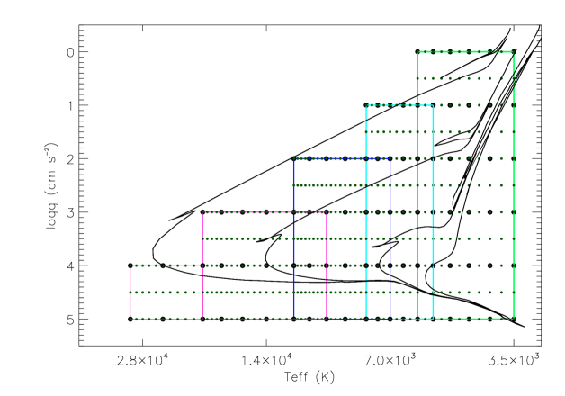
As the effective temperature of the models increases, radiation pressure makes them unstable at low gravity. Accordingly, the smallest value in the range is progressively reduced in the construction of model atmospheres (see Fig. 2 in Mészáros et al. 2012), a feature that our library inherits.
Following the same strategy as in the APOGEE spectral libraries (Zamora et al. 2013; see also Allende Prieto 2009), we split our spectral model collection into five libraries-files according to effective temperature, one for the range 3500–6000 K (), a second for the range 5750–8000 K (), a third for 7000–12,000 K (), a fourth for 10,000–20,000 K (), and a fifth for 20,000–30,000 K ().
A set of coarse libraries with a resolution of is available, and identical files corresponding to and are available as well.444 The libraries are available from the CDS and at ftp://carlos:allende@ftp.ll.iac.es/collection. These only consider three atmospheric parameters (, , and [Fe/H]), and have steps in the parameters that increase with effective temperature: 500 K for the first and the second libraries ( K), 1000 K for the third, 2000 K for the fourth, and 5000 K for the fifth and warmer. All span the metallicity range [Fe/H]. These libraries cover the spectral range between 120 and 6500 nm, sampling the spectra with equidistant steps in ; for the grids the step size is , equivalent to km s-1.
These coarse libraries are useful for some applications, but others will need finer resolution in the parameters. A second set of libraries retains the subdivisions by , and they span the same range in , and [Fe/H], but have much finer steps in the parameters, and include additional dimensions, namely microturbulence (parameterized on a logarithmic scale ) and the [/Fe] abundance ratio. Needless to say, the size of these later libraries-files is much larger than the coarse ones, between a few and tens of gigabytes. Figure 1 illustrates the ranges in the plane - of the libraries. The parameter ranges and step sizes are given in Table 1. These finer libraries are provided only at , with a spectral range between 200 and 2500 nm, and the same equidistant steps in as the smaller libraries. All the libraries give the Eddington flux (first-moment of the radiation field) () at the stellar surface in units of erg cm-2 s-1 Å-1.
| This work | NGSL | |||||
|---|---|---|---|---|---|---|
| star | [Fe/H] | [Fe/H] | ||||
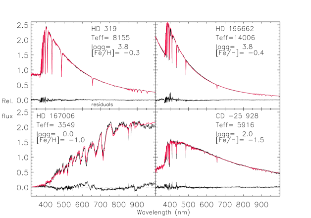
| HD 167006 | 3549 | 0.0 | -1.0 | 3536 | 0.4 | -0.3 |
| CD -25 928 | 5916 | 2.0 | -1.5 | 6426 | 3.0 | -1.2 |
| HD 319 | 8155 | 3.8 | -0.3 | 8195 | 3.9 | -0.4 |
| HD 196662 | 14006 | 3.8 | -0.4 | 14204 | 3.7 | -0.6 |
4 Comparison with observations
A library of model spectra without an assessment of how well it matches reality is useless. We therefore provide in this section several examples of how well the library performs in comparison with a selection of observations. We have chosen to compare the models with data from the second version of the Next Generation Spectral Library (Gregg et al. 2006; Lindler & Heap 2008; Heap & Lindler 2016), which contains low-resolution flux-calibrated observations from the STIS instrument onboard the Hubble Space Telescope.
We selected four representative stars from the library, spanning a reasonable range in , and fitted their STIS spectra with our libraries (the five-parameter version) and the FERRE code (Allende Prieto et al. 2006), which finds by optimization (interpolating in the libraries) the set of parameters that leads to the minimum of the statistics. The library spectra were smoothed to a resolving power of 510 (Bohlin 2007, Allende Prieto & del Burgo 2016). The results are shown in Table 2 and illustrated in Fig. 2. With the exception of CD 928, the agreement between the two sets of effective temperatures is excellent, as one would expect since both analyses fit the same spectral energy distributions. The disagreement for CD 928 is likely related to a difference in surface gravity, which in our analysis is obtained as well from the STIS spectrum, while those provided with the NGSL are tied to the trigonometric parallaxes from Hipparcos. The metallicities show fair agreement.
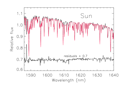
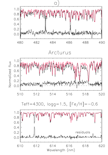
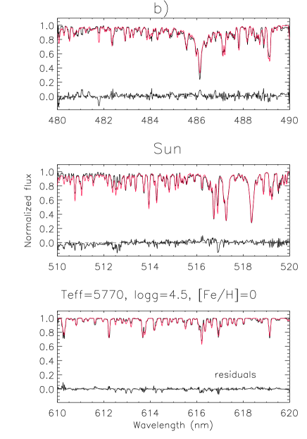
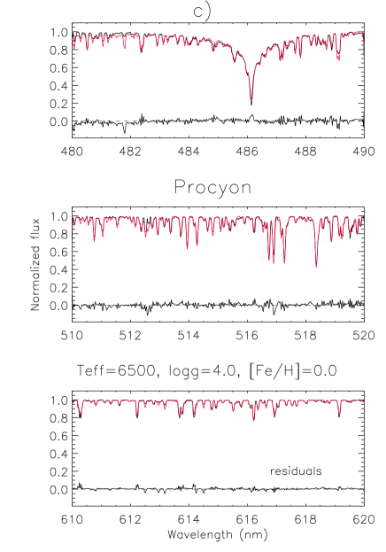
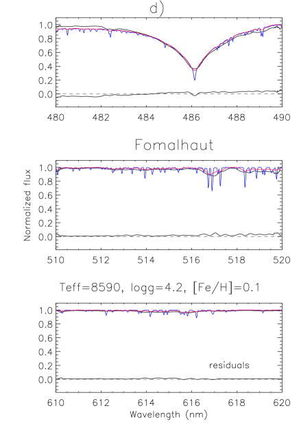
Figure 3 illustrates the comparison between the library and the high resolution spectra of four stars with well-known parameters at high resolving power (). We have chosen three important regions widely used in the literature: the vicinity of H, the region around the Mg I triplet, and the band near the Ca I 616.2 nm transition. The parameters for Arcturus were adopted from Ramírez & Allende Prieto (2011; data from Hinkle et al. 2000), those for Procyon from Allende Prieto et al. (2002; data from Griffin & Griffin 1979), and those for Fomalhaut from Mamajek (2002) and Gáspár et al. (2016; data from Allende Prieto et al. 2004). The solar spectrum is from Kurucz (2005). The main features present in the spectra are captured by the models.
A section of the APOGEE spectrum of solar light reflected off Vesta, smoothed to , is compared to a spectrum interpolated for the solar parameters in Fig. 4. The agreement between data and models in this region is nearly as good as that found in the optical, although the presence of a few missing transitions in the models and residuals caused by imperfectly subtracted OH sky lines are obvious. We note that the H line at 1611 nm is significantly stronger in the model, that is, the situation is the opposite to the case of H, shown in Fig. 3b. Both the observed and model spectra retain their original slope; they have not been continuum normalized but simply divided by their mean values in the selected region. Further comparisons of these models with observations can be found, for example, in Aguado et al. (2017, 2018), Allende Prieto (2016), Allende Prieto & del Burgo (2016), La Barbera et al. (2017), Röck et al. (2017), or Yoakim et al. (2017).
5 Summary and conclusions
The data that enter the construction of model atmospheres and the calculation of synthetic stellar spectra are in constant upgrade, and so are the modeling tools. In this paper we describe a set of calculations that represent our own efforts to improve existing models over more than a decade, and which therefore are, in some ways, already outdated. Nonetheless, these models provide significant advantages over a number of other existing libraries, most notably an extended wavelength coverage and the inclusion of warmer models, and constitute a collection that can be used for practical analysis of stellar spectra or building stellar population models.
The model collection is provided as a set of five separate libraries, each spanning a regular grid in the parameter space. We publish models in which only three parameters are considered (, , and [Fe/H]), with a constant micro-turbulence of 1.5 km s-1, and an abundance ratio [/Fe] that depends on [Fe/H]. We also present additional model libraries in which five parameters are changed ([/Fe] and micro-turbulence, in addition to the previous three). All the libraries are in a format ready to use with the FERRE code555Available from github.com/callendeprieto/ferre. This format is straightforward and has been described in the FERRE documentation.
A comparison with several spectra from the NGSL shows that the models capture the main spectral features and the parameters inferred from the observations are in good agreement with those previously derived by the makers of the NGSL. An in-depth analysis of this library with these models, as well as of the MILES library (Sánchez-Blazquez et al. 2006; Cenarro et al. 2007), will be the subject of future work. The library provides also a reasonable description of stellar spectra at high resolution, as checked against spectra of stars as cool as the K giant Arcturus, or as warm as the A-type star Fomalhaut, and will be systematically used in the analysis of observations from instruments such as SONG (Grundahl et al. 2017) or ESPRESSO (Pepe et al. 2014).
Acknowledgements.
CAP’s research is partially funded by the Spanish MINECO under grant AYA2014-56359-P. PSB acknowledges financial support from the Swedish Research Council and the project grant “The New Milky Way” from the Knut and Alice Wallenberg Foundation. MB acknowledges support from the US National Science Foundation Astronomy and Astrophysics Program (AST- 1313265). SNN acknowledges the support of DOE grant DE-FG52-09NA29580 and NSF grant AST-1312441. We are indebted to the referee of the paper for multiple useful suggestions that improved the quality of the presentation, and to the A&A language editor, Ruth Chester, for an excellent job.References
- Aguado et al. (2018) Aguado, D. S., Allende Prieto, C., González Hernández, J. I., & Rebolo, R. 2018, ApJ, 854, L34
- Aguado et al. (2017) Aguado, D. S., Allende Prieto, C., González Hernández, J. I., Rebolo, R., & Caffau, E. 2017, A&A, 604, A9
- (3) Ali, A. W., & Griem, H. R., 1966, Phys. Rev., 144, 366
- Allende Prieto (2009) Allende Prieto, C. 2009, Astrophysics and Space Science Proceedings, 7, 199
- Allende Prieto et al. (2002) Allende Prieto, C., Asplund, M., García López, R. J., & Lambert, D. L. 2002, ApJ, 567, 544
- Allende Prieto et al. (2004) Allende Prieto, C., Barklem, P. S., Lambert, D. L., & Cunha, K. 2004, A&A, 420, 183
- Allende Prieto et al. (2006) Allende Prieto, C., Beers, T. C., Wilhelm, R., et al. 2006, ApJ, 636, 804
- Allende Prieto & del Burgo (2016) Allende Prieto, C., & del Burgo, C. 2016, MNRAS, 455, 3864
- Allende Prieto et al. (2003) Allende Prieto, C., Hubeny, I., & Lambert, D. L. 2003b, ApJ, 591, 1192
- Allende Prieto et al. (2003) Allende Prieto, C., Lambert, D. L., Hubeny, I., & Lanz, T. 2003a, ApJS, 147, 363
- Allende Prieto (2016) Allende Prieto, C. 2016, A&A, 595, A129
- Allende Prieto & del Burgo (2016) Allende Prieto, C., & del Burgo, C. 2016, MNRAS, 455, 3864
- Asplund (2005) Asplund, M. 2005, ARA&A, 43, 481
- Asplund et al. (2005) Asplund, M., Grevesse, N., & Sauval, A. J. 2005, Cosmic Abundances as Records of Stellar Evolution and Nucleosynthesis, 336, 25
- Badnell et al. (2005) Badnell, N. R., Bautista, M. A., Butler, K., et al. 2005, MNRAS, 360, 458
- La Barbera et al. (2017) La Barbera, F., Vazdekis, A., Ferreras, I., et al. 2017, MNRAS, 464, 3597
- Barklem & Aspelund-Johansson (2005) Barklem, P. S., & Aspelund-Johansson, J. 2005, A&A, 435, 373
- Barklem et al. (1998) Barklem, P. S., O’Mara, B. J., & Ross, J. E. 1998, MNRAS, 296, 1057
- Barklem et al. (2000a) Barklem, P. S., Piskunov, N., & O’Mara, B. J. 2000a, A&AS, 142, 467
- Barklem et al. (2000b) Barklem, P. S., Piskunov, N., & O’Mara, B. J. 2000b, A&A, 363, 1091
- Barklem & O’Mara (1998) Barklem, P. S., & O’Mara, B. J. 1998, MNRAS, 300, 863
- Bautista (1997) Bautista, M. A. 1997, A&AS, 122, 167
- Bautista et al. (1998) Bautista, M. A., Romano, P., & Pradhan, A. K. 1998, ApJS, 118, 259
- Bohlin (2007) Bohlin, R. C. 2007, The Future of Photometric, Spectrophotometric and Polarimetric Standardization, 364, 315
- Bohlin et al. (2017) Bohlin, R. C., Mészáros, S., Fleming, S. W., et al. 2017, AJ, 153, 234
- Cenarro et al. (2007) Cenarro, A. J., Peletier, R. F., Sánchez-Blázquez, P., et al. 2007, MNRAS, 374, 664
- Coelho (2014) Coelho, P. R. T. 2014, MNRAS, 440, 1027
- Feautrier (1963) Feautrier, P. 1963, J. Quant. Spec. Radiat. Transf., 3, 103
- Gáspár et al. (2016) Gáspár, A., Rieke, G. H., & Ballering, N. 2016, ApJ, 826, 171
- Girardi et al. (2004) Girardi L., Grebel E. K., Odenkirchen M., Chiosi C., 2004, A&A, 422, 205
- Girardi et al. (2002) Girardi L., Bertelli G., Bressan A., Chiosi C., Groenewegen M. A. T., Marigo P., Salasnich B., Weiss A., 2002, A&A, 391, 195
- Gregg et al. (2006) Gregg, M. D., Silva, D., Rayner, J., et al. 2006, The 2005 HST Calibration Workshop: Hubble After the Transition to Two-Gyro Mode, 209
- Griffin & Griffin (1979) Griffin, R. F., & Griffin, R. 1979, PASP,
- Grundahl et al. (2017) Grundahl, F., Fredslund Andersen, M., Christensen-Dalsgaard, J., et al. 2017, ApJ, 836, 142
- Gustafsson et al. (1975) Gustafsson, B., Bell, R. A., Eriksson, K., & Nordlund, A. 1975, A&A, 42, 407
- Gustafsson et al. (2008) Gustafsson, B., Edvardsson, B., Eriksson, K., et al. 2008, A&A, 486, 951
- Hauschildt et al. (1997) Hauschildt, P. H., Baron, E., & Allard, F. 1997, ApJ, 483, 390
- Heap & Lindler (2016) Heap, S. R., & Lindler, D. 2016, The Science of Calibration, 503, 211
- Hillier (2012) Hillier, D. J. 2012, From Interacting Binaries to Exoplanets: Essential Modeling Tools, 282, 229
- Hinkle et al. (2000) Hinkle, K., Wallace, L., Valenti, J., & Harmer, D. 2000, Visible and Near Infrared Atlas of the Arcturus Spectrum 3727-9300 A ed. Kenneth Hinkle, Lloyd Wallace, Jeff Valenti, and Dianne Harmer. (San Francisco: ASP) ISBN: 1-58381-037-4, 2000.,
- Hubeny et al. (1994) Hubeny, I., Hummer, D. G., & Lanz, T. 1994, A&A, 282, 151
- (42) Hubeny, I., & Lanz, T., SYNSPEC – A User’s Guide, version 43, available from http://nova.astro.umd.edu/Tlusty2002/pdf/syn43guide.pdf
- Hubeny & Lanz (1995) Hubeny, I., & Lanz, T. 1995, ApJ, 439, 875
- Hubeny & Lanz (2017) Hubeny, I., & Lanz, T. 2017, arXiv:1706.01859
- Hummer et al. (1993) Hummer, D. G., Berrington, K. A., Eissner, W., et al. 1993, A&A, 279, 298
- Husser et al. (2013) Husser, T.-O., Wende-von Berg, S., Dreizler, S., et al. 2013, A&A, 553, A6
- Hutchinson et al. (2016) Hutchinson, T. A., Bolton, A. S., Dawson, K. S., et al. 2016, AJ, 152, 205
- Irwin (1981) Irwin, A. W. 1981, ApJS, 45, 621
- Koesterke (2009) Koesterke, L. 2009, American Institute of Physics Conference Series, 1171, 73
- Koesterke et al. (2008) Koesterke, L., Allende Prieto, C., & Lambert, D. L. 2008, ApJ, 680, 764-773
- Korn (2008) Korn, A. J. 2008, Physica Scripta Volume T, 133, 014009
- Kurucz (1979) Kurucz, R. L. 1979, ApJS, 40, 1
- Kurucz (2005) Kurucz, R. L. 2005, Memorie della Societa Astronomica Italiana Supplementi, 8, 189
- Lee & Kim (2004) Lee, H.-W., & Kim, H. I. 2004, MNRAS, 347, 802
- Lanz & Hubeny (2007) Lanz, T., & Hubeny, I. 2007, ApJS, 169, 83
- (56) Lindler D. J., Heap S. R., 2008, STIS Next Generation Spectral Library (v1), documentation available at http://archive.stsci.edu/pub/hlsp/stisngsl/aaareadme.pdf
- (57) Ludwig, H.-G., Koesterke, L., Allende Prieto, C., Bertrán de Lis, S., Freytag, B., & Caffau, E. 2018, A&A submitted
- Majewski et al. (2017) Majewski, S. R., Schiavon, R. P., Frinchaboy, P. M., et al. 2017, AJ, 154, 94
- Mamajek (2012) Mamajek, E. E. 2012, ApJ, 754, L20
- Mészáros et al. (2012) Mészáros, S., Allende Prieto, C., Edvardsson, B., et al. 2012, AJ, 144, 120
- Nahar (1995) Nahar, S. N. 1995, A&A, 293, 967
- (62) The Opacity Project Team .The Opacity Project, Vol 1, 1995, Vol. 2, 1996, Institute of Physics Publishing
- Palacios et al. (2010) Palacios, A., Gebran, M., Josselin, E., et al. 2010, A&A, 516, A13
- Pepe et al. (2014) Pepe, F., Molaro, P., Cristiani, S., et al. 2014, Astronomische Nachrichten, 335, 8
- Puls et al. (1996) Puls, J., Kudritzki, R.-P., Herrero, A., et al. 1996, A&A, 305, 171
- Ramírez & Allende Prieto (2011) Ramírez, I., & Allende Prieto, C. 2011, ApJ, 743, 135
- Recio-Blanco et al. (2016) Recio-Blanco, A., de Laverny, P., Allende Prieto, C., et al. 2016, A&A, 585, A93
- Röck et al. (2017) Röck, B., Vazdekis, A., La Barbera, F., et al. 2017, MNRAS, 472, 361
- Sánchez-Blázquez et al. (2006) Sánchez-Blázquez, P., Peletier, R. F., Jiménez-Vicente, J., et al. 2006, MNRAS, 371, 703
- (70) Schwenke, D. W. 1998, Faraday Discussions, 109, 321
- Seaton et al. (1994) Seaton, M. J., Yan, Y., Mihalas, D., & Pradhan, A. K. 1994, MNRAS, 266, 805
- Starkenburg et al. (2017) Starkenburg, E., Martin, N., Youakim, K., et al. 2017, MNRAS, 471, 2587
- Stehle (1994) Stehle, C. 1994, A&AS, 104, 509
- Stehlé & Hutcheon (1999) Stehlé, C., & Hutcheon, R. 1999, A&AS, 140, 93
- (75) Cunto, W., Mendoza, C., Ochsenbein, F., Zeippen, C.J., 1993, A&A, 275, L5. (TOPbase at http://cdsweb.u-strasbg.fr/topbase/topbase.html)
- Trampedach et al. (2013) Trampedach, R., Asplund, M., Collet, R., Nordlund, Å., & Stein, R. F. 2013, ApJ, 769, 18
- Tremblay et al. (2013) Tremblay, P.-E., Ludwig, H.-G., Freytag, B., Steffen, M., & Caffau, E. 2013, A&A, 557, A7
- Tsuji (1964) Tsuji, T. 1964, Annals of the Tokyo Astronomical Observatory, 9, 1
- Tsuji (1973) Tsuji, T. 1973, A&A, 23, 411
- Tsuji (1976) Tsuji, T. 1976, PASJ, 28, 543
- Van Eck et al. (2017) Van Eck, S., Neyskens, P., Jorissen, A., et al. 2017, A&A, 601, A10
- Vidal et al. (1970) Vidal, C. R., Cooper, J., & Smith, E. W. 1970, J. Quant. Spec. Radiat. Transf., 10, 1011
- Vidal et al. (1973) Vidal, C. R., Cooper, J., & Smith, E. W. 1973, ApJS, 25, 37
- Youakim et al. (2017) Youakim, K., Starkenburg, E., Aguado, D. S., et al. 2017, MNRAS, 472, 2963
- Zamora et al. (2015) Zamora, O., García-Hernández, D. A., Allende Prieto, C., et al. 2015, AJ, 149, 181