Does black-hole growth depend on the cosmic environment?
Abstract
It is well known that environment affects galaxy evolution, which is broadly related to supermassive black hole (SMBH) growth. We investigate whether SMBH evolution also depends on host-galaxy local (sub-Mpc) and global ( Mpc) environment. We construct the surface-density field (local environment) and cosmic web (global environment) in the COSMOS field at . The environments in COSMOS range from the field to clusters (), covering the environments where of galaxies in the Universe reside. We measure sample-averaged SMBH accretion rate () from X-ray observations, and study its dependence on overdensity and cosmic-web environment at different redshifts while controlling for galaxy stellar mass (). Our results show that does not significantly depend on overdensity or cosmic-web environment once is controlled, indicating that environment-related physical mechanisms (e.g. tidal interaction and ram-pressure stripping) might not significantly affect SMBH growth. We find that is strongly related to host-galaxy , regardless of environment.
keywords:
galaxies: evolution – large-scale structure of Universe – galaxies: active – galaxies: nuclei – quasars: supermassive black holes – X-rays: galaxies1 Introduction
The environments of galaxies play a crucial role in their evolution (e.g. De Lucia et al., 2006; Conselice, 2014; Somerville & Davé, 2015). In the local universe, denser regions are preferentially populated by early-type quiescent galaxies, while less-dense regions are more likely to host late-type star-forming galaxies (e.g. Dressler, 1980; Balogh et al., 2004; Kauffmann et al., 2004). This environmental dependence of star-forming/quiescent types exists at , although it is less clear at higher redshifts (e.g. Cooper et al., 2006; Elbaz et al., 2007; Peng et al., 2010; Scoville et al., 2013; Darvish et al., 2016).
Several possible environment-related mechanisms could affect galaxy evolution. Cold gas, the fuel of star formation, could flow into galaxies through cosmic filaments (e.g. Kereš et al., 2005; Dekel et al., 2009); frequent tidal interactions in denser regions could effectively deplete cold gas (e.g. Farouki & Shapiro 1981; Moore et al. 1998); the strong ram pressure in clusters can strip cold gas from galaxies and suppress subsequent star formation (e.g. Gunn & Gott 1972; Ebeling et al. 2014; Poggianti et al. 2016); and mergers, which can fundamentally change galaxy properties, happen more frequently in high-density regions (e.g. Hopkins et al., 2006; Lin et al., 2010). These physical processes might also affect active galactic nucleus (AGN) activity, as the growth of supermassive black holes (SMBHs) also relies on the supply of cold gas (e.g. Alexander & Hickox, 2012; Vito et al., 2014; Poggianti et al., 2017).
Optical observations of low-redshift () quasars disagree on whether they tend to reside in high-density or low-density regions compared to normal galaxies (e.g. Serber et al. 2006; Strand et al. 2008; Lietzen et al. 2009). This disagreement might be caused if these works did not carefully control for host-galaxy properties. Karhunen et al. (2014) found quasars do not show a significant dependence on environment compared to normal galaxies with matched redshift and host-galaxy luminosities. At high redshift (), optical observations are limited to rare luminous quasars, and deep spectroscopic observations are often needed to measure their environment. Therefore, these studies are often limited to small sample sizes and statistically significant conclusions cannot be obtained (e.g. Bañados et al., 2013; Overzier, 2016; Balmaverde et al., 2017).
Optical selection is often biased to luminous broad-line (BL) quasars, especially at high redshift. These BL quasars are rare and not well representative of the whole AGN population. X-ray emission can trace AGN activity down to a modest level and is widely used to investigate SMBH growth over the majority of cosmic history (e.g. Brandt & Alexander, 2015; Xue, 2017). Studies of AGN activity vs. environment found that, at low redshift (), the X-ray AGN fraction in rare rich clusters is generally lower than that in the field (e.g. Martini et al. 2009; Ehlert et al. 2014; but also see, e.g. Haggard et al. 2010). At higher redshifts, relevant studies are often constrained to rare protoclusters with limited AGN/galaxy sample sizes. Their results suggest that AGN activity tends to be enhanced in these protoclusters (e.g. Lehmer et al. 2009; Digby-North et al. 2010; Lehmer et al. 2013; Martini et al. 2013; Umehata et al. 2015; Alexander et al. 2016; but also see Macuga et al. 2018).
However, this apparent environmental dependence might only be a secondary effect, and SMBH growth might be more fundamentally related to host-galaxy properties which are themselves related to environment. For example, X-ray AGN activity is strongly related to host-galaxy stellar mass () rather than color (e.g. Xue et al. 2010) or star-formation rate (SFR; e.g. Yang et al. 2017), and thus must be carefully controlled when assessing AGN dependence on other host-galaxy properties. On the other hand, massive galaxies tend to reside in high-density regions (e.g. Coil et al., 2006, 2017). Therefore, to avoid such -related biases, a large sample of AGNs and galaxies is needed to investigate the accretion-environment relation while controlling for host-galaxy .
In this paper, we study the dependence of sample-averaged SMBH accretion rate () on galaxy overdensity and cosmic-web environment while controlling for . The sample-averaged SMBH accretion is employed to approximate long-term average SMBH accretion for a galaxy sample (e.g. Chen et al., 2013; Hickox et al., 2014; Yang et al., 2017, 2018), because AGNs plausibly have strong variability on timescales of yr (e.g. Martini & Schneider, 2003; Novak et al., 2011; Sartori et al., 2018). Here, we define the overdensity as the galaxy surface number density relative to the median value at a given redshift and cosmic-web environment as a galaxy’s association to the field, a filament, or a cluster. The overdensity and cosmic-web environment are assessed on physical scales of sub-Mpc and Mpc, respectively. Hereafter, we refer to overdensity and cosmic-web environment as “local” and “global” environments, respectively.
Our aim is to probe a wide redshift range of with large samples of X-ray AGNs () and galaxies (). In particular, this range covers , the peak of cosmic AGN and star-formation activity, when various physical processes such as galaxy mergers and AGN feedback likely play an important role in shaping SMBH and galaxy coevolution (e.g. Conselice, 2014; Madau & Dickinson, 2014; Brandt & Alexander, 2015; King & Pounds, 2015).
Our analyses are based on the Cosmic Evolution Survey (COSMOS; e.g. Scoville et al., 2007; McCracken et al., 2012). COSMOS has been intensively covered by spectroscopic and multiwavelength imaging observations (e.g. Lilly et al., 2009; Laigle et al., 2016). Over 20,000 sources have secure spectroscopic redshifts (spec-) while other sources have reliable photometric redshifts (photo-) derived from high-quality UV-to-IR data (up to 32 bands; e.g. Laigle et al. 2016). The UV-to-IR data also make it possible to assess host-galaxy properties such as and star-forming/quiescent type (e.g. Ilbert et al. 2013; Davidzon et al. 2017). Deep Chandra X-ray observations ( 160 ks exposure), which can be used to measure SMBH growth, are also available from the COSMOS-Legacy survey (Civano et al., 2016). The excellent X-ray positions from Chandra () enables reliable matching between X-ray and optical sources (Marchesi et al., 2016a).
Thanks to its relatively large area ( deg2) and deep panchromatic coverage, COSMOS is one of the major fields for environment studies. State-of-the-art techniques have been applied to COSMOS to derive reliable measurements of the surface-density field up to (e.g. Scoville et al., 2013; Darvish et al., 2015). The statistical properties of the resulting density field such as mean densities and density ranges agree with the predictions from cosmological simulations (e.g. Scoville et al., 2013). Based on the density field, Darvish et al. (2017) utilized a new technique to construct a measurement of the cosmic web (Aragón-Calvo et al., 2007). This method allows the mapping of sources to clusters, filaments, and the field.
This paper is structured as follows. In §2, we describe our data analyses. In §3, we present our results. We discuss our results in §4 and summarize our study in §5.
Throughout this paper, we assume a cosmology with km s-1 Mpc-1, , and , and a Chabrier initial mass function (Chabrier, 2003). Quoted uncertainties are at the (68%) confidence level, unless otherwise stated. We express , , and (halo mass) in units of and in units of yr-1. indicates AGN X-ray luminosity at rest-frame 2–10 keV and is in units of erg s-1. All lengths/distances are in physical (proper) scale, unless otherwise stated.
2 Data Analyses
2.1 Galaxy Sample Selection
Our data are based on the COSMOS2015 survey (Laigle et al., 2016). We only utilize sources within both the COSMOS and UltraVISTA regions, and remove objects in masked regions (e.g. bad pixels in detectors). These sources cover an area of deg2 (see Fig. 1 and Tab. 7 in Laigle et al. 2016). The UltraVISTA region has deep NIR imaging data that are essential in estimating photo- and (§2.2). We restrict our study to the sources brighter than (the limiting magnitude of the COSMOS2015 catalog) to avoid large uncertainties of photo- for faint sources. The basic properties of our sample are listed in Tab. 1. Our analyses (§3) are performed for the three redshift bins (, 1.2–2, and 2–3) listed in Tab. 1. These redshift bins cover comoving volumes of Mpc3, Mpc3, and Mpc3, respectively. Tab. 2 shows a portion of our source catalogs, and the full version is available as supplementary material.
We obtain spec- for sources in our sample (see Tab. 1; Marchesi et al. 2016a; Delvecchio et al. 2017; Salvato et al. in prep.).111In the late stages of this work, a new spec- data set, the DEIMOS 10k catalog, was released (Hasinger et al., 2018). This catalog could increase our spec- sample by , unlikely to affect our qualitative results. For sources without spec-, we adopt the photo- measurements from the COSMOS2015 catalog. These measurements are derived from high-quality UV-to-NIR photometric data including 18 broad bands, 12 medium bands, and 2 narrow bands (see Tab. 1 in Laigle et al. 2016). The medium bands can effectively improve the photo- quality, enabling reliable environment studies in COSMOS (e.g. Darvish et al. 2015; Darvish et al. 2017). When compared to different spec- catalogs, the photo- have and outlier () fraction (see Tab. 5 in Laigle et al. 2016), where is defined as ) (e.g. Yang et al. 2014). When compared with the recently released DEIMOS 10k spec- catalog (Hasinger et al., 2018), the COSMOS2015 photo- have and , further demonstrating the high photo- quality of the COSMOS2015 catalog. We consider all galaxies (including X-ray detected and undetected) when deriving (see §2.4).
| Redshift | / | FracQ | (keV) | ||||||||
|---|---|---|---|---|---|---|---|---|---|---|---|
| (1) | (2) | (3) | (4) | (5) | (6) | (7) | (8) | (9) | (10) | (11) | (12) |
| 0.3–1.2 | 94,152/18,099 | 0.011 | 2% | 9.3 | 13% | 180 | (,0.18) | 38,840/ 48,960/ 6,352 | 889 | (0.9,12.5) | (42.6,43.3) |
| 1.2–2.0 | 48,981/1,322 | 0.020 | 3% | 9.8 | 7% | 80 | (,0.13) | 20,365/ 28,616/ – | 701 | (1.3,17.7) | (43.3,43.9) |
| 2.0–3.0 | 22,828/412 | 0.059 | 10% | 9.9 | 2% | 50 | (,0.13) | 14,265/ 8,563/ – | 429 | (1.7,23.6) | (43.7,44.2) |
Note. — (1) Redshift bins. (2) Numbers of galaxies and spec- sources in our sample (). (3) Photo- uncertainty (compared to spec-). (4) Photo- outlier fraction. (5) Median stellar mass. (6) Fraction of quiescent galaxies. (7) Number of -slices. (8) The overdensity (25%,75%) percentile range. (9) Number sources in the field/filament/cluster environments. We do not assign cluster environment at due to its generally weak signals (see §2.3.2). (10) Number of X-ray detected sources. (11) Rest-frame X-ray energy sampled at median redshift. (12) The (25%,75%) percentile range of for X-ray detected sources.
| RA | DEC | Typegal | Web | |||||||
|---|---|---|---|---|---|---|---|---|---|---|
| (1) | (2) | (3) | (4) | (5) | (6) | (7) | (8) | (9) | (10) | (11) |
| 149.411496 | 2.712315 | 22.8 | 0.706 | 0.655 | 0.774 | 9.18 | 1 | 2 | ||
| 149.411504 | 2.765237 | 23.5 | 0.975 | 0.951 | 0.990 | 8.06 | 1 | 2 | ||
| 149.411576 | 2.336084 | 21.0 | 1.783 | 1.729 | 1.818 | 11.22 | 1 | 1 | ||
| 149.411578 | 2.306681 | 21.3 | 1.359 | 1.241 | 1.433 | 10.71 | 0 | 1 | ||
| 149.411581 | 2.411649 | 21.5 | 0.389 | 0.381 | 0.398 | 9.28 | 1 | 1 | ||
| 149.411603 | 2.243533 | 21.9 | 1.502 | 1.469 | 1.543 | 10.32 | 1 | 1 | ||
| 149.411643 | 2.290855 | 23.6 | 1.185 | 1.171 | 1.198 | 9.07 | 1 | 1 | ||
| 149.411643 | 2.592744 | 23.6 | 0.880 | 0.825 | 0.942 | 9.24 | 1 | 1 | ||
| 149.411659 | 2.319370 | 23.6 | 1.022 | 0.812 | 1.148 | 9.23 | 1 | 2 | ||
| 149.411661 | 2.410365 | 22.5 | 1.063 | 1.063 | 1.063 | 9.11 | 1 | 1 |
Note. — Only a portion of this table is shown here, and the full version is available as supplementary materials. The table is sorted in ascending order of RA. (1) & (2) Source J2000 coordinates. (3) AB magnitude from the COSMOS2015 catalog (Laigle et al., 2016). (4), (5), & (6) Redshift and redshift 1 lower and upper limits (§2.1). For spec- sources, the lower and upper limits are set the same as the redshift value. (7) Stellar mass (§2.2). (8) Galaxy type (0: quiescent; 1: star-forming; §2.2). (9) Overdensity (§2.3.1). (10) Cosmic-web environment (0: cluster; 1: filament; 2: field; §2.3.2). We do not assign cluster environment at due to its generally weak signals. (11) X-ray luminosity (rest-frame 2–10 keV; §2.4.1). For X-ray undetected sources, the values are set to “”.
2.2 Stellar Mass
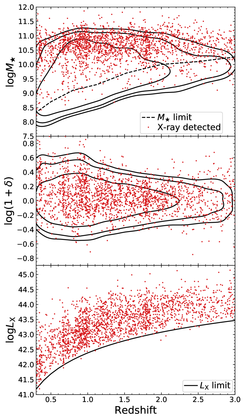
To estimate , we perform spectral energy distribution (SED) fitting with cigale (Noll et al., 2009; Serra et al., 2011) at or (§2.1). The input photometry is from the COSMOS2015 catalog (§2.1). We do not adopt the measurements from the COSMOS2015 catalog directly, mainly because the our redshifts are not exactly the same as those in the COSMOS2015 catalog (§2.1). We employ nebular and dust emission in cigale (Noll et al., 2009; Draine & Li, 2007). We apply the extinction law from Calzetti et al. (2000) with ranging from . Following Yang et al. (2018), we use a model of the star formation history (SFH) with ranging from 8 to 10.5. We allow stellar metallicity values of , where is the mass fraction of metals. Our measurements have a systematic of 0.002 dex and a scatter of 0.11 dex compared to those in the COSMOS2015 catalog. For the 239 BL AGNs (identified by Marchesi et al. 2016a), we also adopt an additional BL AGN component following the settings in Tab. 1 of Ciesla et al. (2015). The resulting values are typically dex different from those obtained with only galaxy templates (see § 2.1.3 of Yang et al. 2018). Fig. 1 displays vs. redshift for our sample. We also show the completeness limit corresponding to from Laigle et al. (2016) in Fig. 1. The completeness limit is estimated based on an empirical method which does not assume a specific galaxy template. The limiting at , 2, and 3 are 9.3, 10.0, and 10.3, respectively. In §3, we perform analyses for above these limits in three redshift bins of , 1.2–2, and 2–3, respectively.
We classify a source as a quiescent galaxy if its rest-frame colors satisfy and , otherwise we classify it as a star-forming galaxy (Williams et al., 2009; Ilbert et al., 2010).222Here, the NUV specifically refers to the GALEX band centered at 2300 Å. Here, the rest-frame colors are obtained from our SED fitting. This color-based selection helps to avoid misclassifying dust-reddened star-forming galaxies as quiescent galaxies (e.g. Ilbert et al., 2010, 2013). The fractions of quiescent galaxies in different redshift ranges are listed in Tab. 1. This classification is used to estimate X-ray emission from X-ray binaries (XRBs; see §2.4.3). Our color-color scheme is not appropriate for galaxies hosting BL AGNs due to the strong AGN UV-to-NIR emission. Following Yang et al. (2017), we set the hosts of BL AGNs as star-forming galaxies. Setting them as either star-forming or quiescent galaxies has negligible effects to our results, as BL AGNs are only a small population compared to the entire galaxy sample ().
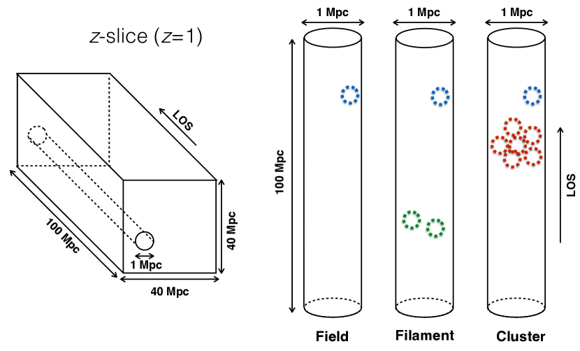
2.3 Environment
We build the surface-density field and cosmic-web estimates in this section. The technical details are presented in Darvish et al. (2015); Darvish et al. (2017), and we briefly describe the procedures in §2.3.1 and §2.3.2. In Appendix A, we explain our environment measurements in a straightforward way, especially for readers who are not familiar with environmental studies. As demonstrated in §4.1, the physical environment-SFR relation clearly exists in our sample, supporting the robustness of our environment measurements.
Some studies suggest that there might be different environmental effects for “central” vs. “satellite” galaxies in a dark-matter halo (e.g. Li et al. 2006; Hickox et al. 2009). We do not label our sources as central or satellite galaxies, because most galaxies () at low redshift () are observed to be isolated or reside in small groups (galaxy members ) and their central/satellite classification is challenging due to factors like photo- uncertainties and survey sensitivity (e.g. Knobel et al. 2009, 2012). At higher redshift, the fraction of isolated or small-group galaxies is even higher as the large-scale structure is still in development (e.g. Springel et al. 2005; Overzier 2016). Considering that our sources cover a wide redshift range of , a detailed unbiased central/satellite classification is beyond the scope of this work.
2.3.1 Density Field (Local Environment)
We adopt the “weighted adaptive kernel smoothing” method to construct the surface-density field that probes sub-Mpc physical scales. As demonstrated by intensive simulations, the performance of this method is excellent (see §5 and §6 of Darvish et al. 2015). The density field is calculated for all sources, including normal galaxies and X-ray detected sources.
We first calculate as a function of redshift. is derived within at each redshift. is at low redshift () and rises to toward high redshift (). This level of photo- accuracy is sufficient for reliable cosmic-environment characterization (e.g. Scoville et al. 2013; Darvish et al. 2015). We then define a series of redshift slices (-slices) with widths of . This width is suggested by Malavasi et al. (2016). The -slices are designed in a way that of each -slice is overlapping with its next -slice. Such dense design is to appropriately consider the photo- distribution of galaxies close to the boundaries of each -slice (see §3.1 of Darvish et al. 2015). The numbers of -slices in different redshift ranges are listed in Tab. 1. For each -slice, we calculate the weight for each source, defined as the percentage of the redshift probability distribution function within this -slice. We assign a weight of 100% to sources with available spectroscopic redshifts. To reduce computational time, at each redshift, we only include sources with weight at least 10%. To derive the surface-density field for each -slice, we utilize a 2D Gaussian kernel whose width adaptively decreases in denser regions, ranging from Mpc (1% percentile) to Mpc (99% percentile). The algorithm requires an input “global smoothing width”. We adopt the value of 0.5 Mpc which is the typical virial radius of X-ray clusters in COSMOS (; e.g. Finoguenov et al. 2007; George et al. 2011).333Darvish et al. (2015) tested global smoothing widths from 0.1 to 2.0 Mpc and did not find a significant change in the resulting density field. Following Darvish et al. (2017), we filter out sources near ( Mpc) the edge of the field and/or large masked regions in the COSMOS2015 survey (Laigle et al., 2016), because density measurements for these sources are unreliable. The procedures above yield measurements of surface number density (, in units of Mpc-2) for each source.
We quantify the local environment for each source via the dimensionless overdensity parameter, defined as
| (1) |
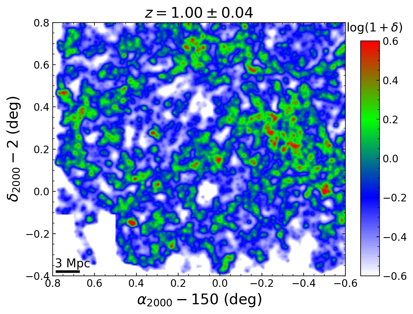
where is the median at each redshift. To minimize the effects of cosmic variance, is calculated within at redshift . Figs. 2 and 3 show the overdensity maps for two -slices centered at and 2.0, respectively. The above overdensity measurements are based on sources with (see §2.1).
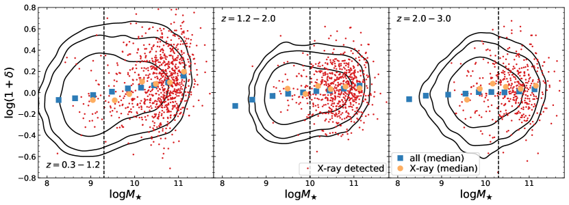
Figs. 1 and 4 show overdensity as a function of redshift and , respectively (see Tab.1 for typical overdensity ranges of our sample). There are positive trends between overdensity and at , consistent with previous work (e.g. Darvish et al., 2017).
In our overdensity estimation above, we have appropriately weighted sources according to their photo- uncertainties (see §2.3). However, this weighting technique does not account for catastrophic photo- outliers. The outlier fractions are , when compared with different spec- catalogs (see §2.1 and Tab. 1). The photo- outliers increase the noise level in the derivation of density field. Darvish et al. (2015) assessed the effects of outliers via simulations (see their §5.1). They concluded that an outlier fraction of 10% has little effect on the derived density field. Therefore, our results should not be qualitatively affected by the photo- outliers.
The typical stellar mass of our sample is relatively small (; see Tab. 1). We have also tested using only a subsample of galaxies when estimating the density field. Our results (§3) do not change qualitatively. The total stellar mass included in this subsample is of that included in the entire sample. However, the subsample consists of only of our sources, inevitably leading to stronger Poisson noise in the density-field estimation.
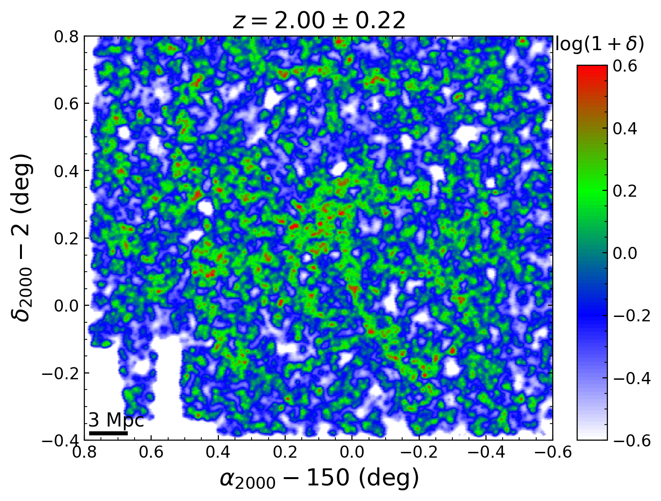
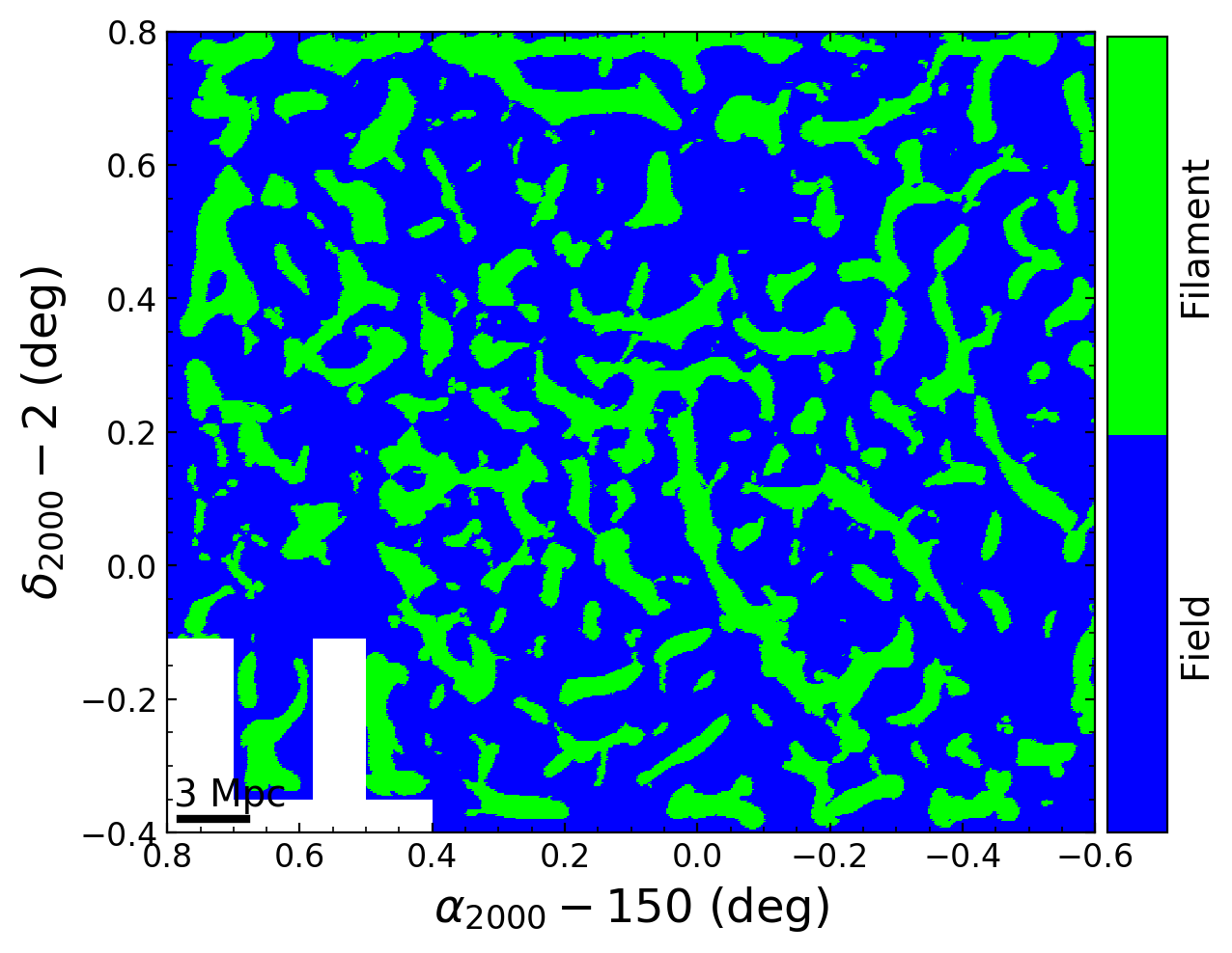
2.3.2 Cosmic Web (Global Environment)
Based on the density field derived in §2.3.1, we extract a cosmic-web estimate with the multi-scale morphology filter (MMF) algorithm (e.g. Aragón-Calvo et al., 2007; Darvish et al., 2014; Darvish et al., 2017). The basic idea is to measure the geometry of the density field around each point in the -slice. If the geometry is similar to that of a typical cluster/filament, then the point’s environment is classified as cluster/filament; otherwise it is classified as the field.
Specifically, we first derive the Hessian matrix (second-order partial derivatives) of the density field for each point in a -slice (see §3.4.1 of Darvish et al. 2017 for details). We then calculate two eigenvalues for each Hessian matrix. The eigenvalues describe the density-field geometry around the point. Based on the signs, ratios, and normalizations of the two eigenvalues, a cluster signal () and a filament signal () are obtained for the point. Here, the signals are two numbers within , where larger values indicate higher chances of lying in a cluster/filament. To account for the multi-scale nature of clusters and filaments, the above procedures are repeated but each time the density field is smoothed with a Gaussian kernel of different physical scales (0.25, 0.50, 0.75, 1.00, 1.50, 2.00 Mpc). The final cluster/filament signal for each point is assigned as the largest value among those obtained with different smoothing scales.
After obtaining the signal maps for each -slice, we need to apply appropriate signal thresholds to identify clusters and filaments. A higher signal threshold generally increases reliability but decreases completeness in structure selection. We adopt the redshift-dependent thresholds from §3.4.2 of Darvish et al. (2017), which are designed to balance between reliability and completeness. These thresholds are (cluster) and (filament). Following Darvish et al. (2017), we assign a cluster environment to a point if it has and . If a point is not assigned as a cluster environment but has , we assign it as a filament environment. If an object is not assigned as cluster or filament environment, we assign it as the field environment.
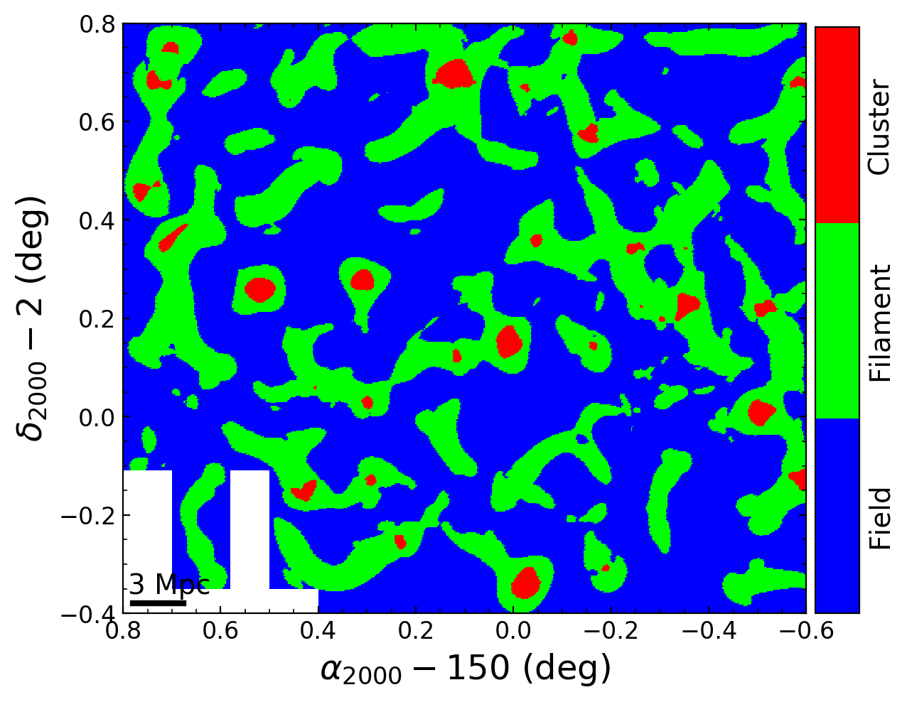
The above criterion has been successfully applied to sources (e.g. Darvish et al., 2017). Fig. 2 shows the cosmic-web map for the -slice centered at . The clusters are roughly round with typical physical sizes of Mpc. The filaments are elongated, with a typical length of Mpc. However, we find, at , the clusters are often dominated by noise. This is understandable as clusters are still forming at high redshifts and they exist in the form of protoclusters (e.g. Kravtsov & Borgani, 2012; Overzier, 2016). The protoclusters have weaker signals and are generally beyond our detection sensitivity. Therefore, we do not assign cluster environments for redshift ranges of and . Specifically, if an object at has , we assign it as a filament environment; otherwise, we assign it as a field environment. Fig. 3 displays the cosmic-web map for the -slice centered at . The numbers of sources associated with different cosmic-web environments are summarized in Tab. 1.
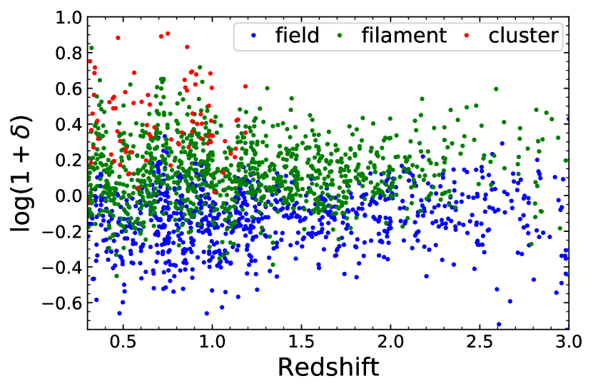
Fig. 5 shows the overdensity as a function of redshift for different cosmic-web environments. Although the overdensity generally rises from the field to clusters, there are substantial overlapping areas in the overdensity-redshift parameter space. This overlap is understandable as the overdensity and cosmic-web measurements describe cosmic environment on different scales (sub-Mpc vs. Mpc). The overlap highlights the importance of our MMF algorithm in the construction of the cosmic web, and a simple overdensity-based algorithm would not be feasible for cosmic-web association. Readers might worry that the overlap might smear out potentially weak trends between and environment. However, this is not an issue in our analyses, because we assess dependence on both overdensity and cosmic-web environment individually and reach consistent results (see §3).
George et al. (2011) have associated galaxies with X-ray selected clusters at using a probabilistic method. We match their cluster-member candidates (member probability above 70%) to our sample with a matching radius. As expected, the 1,851 matched galaxies generally have high overdensity values of (25%–75% percentile) compared to our overall sample (see Tab. 1). For these 1,851 galaxies, 44% and 50% are assigned as cluster and filament, respectively, in our catalog. The 44% filament objects tend to lie in the boundary between clusters and filaments in our -slices, where the cluster/filament classification is sensitive to the methodology. The other 6% of galaxies are assigned as the field environment in our catalog. This disagreement is likely caused by the differences in adopted redshift measurements, as these galaxies’ redshift values in the two catalogs differ by . In comparison, the other 94% of galaxies (George et al. 2011 cluster candidates assigned as cluster/filament galaxies) have redshift differences of only . Our adopted photo- values should have improved quality compared to those adopted in George et al. (2011), who used photo- from an earlier COSMOS catalog (Ilbert et al., 2009). Note that it is natural that most of our cluster galaxies are not identified by George et al. (2011), because their X-ray selected clusters are not complete.
2.4 Black Hole Accretion Rate
We derive for samples of sources broadly following the procedures in §2.3 of Yang et al. (2017). Briefly, we first calculate the total sample-averaged () considering both X-ray detected sources (§2.4.1) and undetected sources (§2.4.2). The undetected sources are considered with an X-ray stacking technique. The stacking procedure is necessary to avoid biases due to the limited X-ray survey sensitivity, as faint AGNs become undetected toward high redshift. We obtain the AGN by subtracting the component contributed by XRBs (§2.4.3). Finally, we convert AGN to in units of yr-1.
2.4.1 X-ray Detected Sources
We select all X-ray detected sources using the COSMOS-Legacy X-ray survey (Civano et al., 2016). The COSMOS-Legacy survey, conducted by Chandra, is the deepest X-ray survey available for COSMOS, and can sample most of cosmic accretion power. For instance, at , the peak of cosmic AGN activity, it covers ranging from times below the knee luminosity of the X-ray luminosity function to times above the knee luminosity, corresponding to of the total (integrated from the X-ray luminosity function).
There are 2,020 X-ray sources matched to the optical/NIR COSMOS2015 catalog based on a likelihood-ratio technique by Marchesi et al. (2016a, see Tab. 1). Most () of these X-ray sources should be AGNs considering their relatively high X-ray luminosity (; e.g. Xue et al. 2016; Luo et al. 2017). Besides the BL AGNs, there are X-ray sources with spec- measurements (see §2.1). We use these non-BL X-ray sources to assess the photo- quality for the X-ray sources with only photo- measurements, because Yang et al. (2018) estimated most () of the photo- sources should be non-BL AGNs. The photo- have and (see 2.1), comparable to the AGN photo- quality in the literature (e.g. Luo et al., 2010; Hsu et al., 2014; Yang et al., 2014).
A source might be detected in multiple X-ray bands. In this case, we choose, in order of priority, hard-band (2–7 keV), full-band (0.5–7 keV), and soft-band (0.5–2 keV) fluxes, for the calculation below. This order of detection bands is to minimize the effects of X-ray obscuration. The fractions of X-ray sources with fluxes from the hard, full, and soft bands are 63%, 34%, and 3%, respectively.
The X-ray fluxes in the COSMOS-Legacy catalog are only corrected for Galactic absorption. Marchesi et al. (2016a) have estimated intrinsic absorption column densities () based on hardness ratios. We do not apply these absorption corrections, because the majority () of sources have poorly constrained values (consistent with zero at a 90% confidence level) mainly due to limited numbers of counts. Instead, we evaluate the level of absorption corrections for COSMOS-like sources using the ultradeep 7 Ms catalog of the Chandra Deep Field-South (CDF-S; Luo et al. 2017). Such sources have 44 times more counts in CDF-S than COSMOS and absorption corrections have been estimated individually (e.g. Yang et al. 2016; Liu et al. 2017; Luo et al. 2017). These COSMOS-like sources are selected via applying the COSMOS flux limits (Civano et al., 2016) to CDF-S. We find that these COSMOS-like sources have a median absorption correction factor (intrinsic flux divided by observed flux) of . The corresponding uncertainty caused by absorption correction is generally smaller than the statistical uncertainties of (§2.4.3), and thus absorption should not bias our conclusions. The relatively low level of absorption corrections is mainly due to our choice of bands. Another reason is that we can sample ultra-hard ( keV, rest-frame) penetrating X-rays for most sources (see Tab. 1).
We convert the X-ray fluxes to assuming a power-law model with a photon index of , which is the typical intrinsic slope of distant AGNs (e.g. Marchesi et al. 2016b; Yang et al. 2016; Liu et al. 2017). Our conclusions do not change if we adopt a slightly different value (e.g. ). The resulting values as a function of redshift are displayed in Fig. 1 (also see Tab. 1 for typical ranges). Fig. 1 also shows the estimated limit, assuming a 0.5–10 keV flux threshold of erg cm-2 s-1 (Civano et al., 2016).
2.4.2 X-ray Undetected Sources
We perform X-ray stacking to calculate for X-ray undetected sources in our samples. We use the full-band X-ray data. The full band is the most sensitive in the sense that it detects the largest number of X-ray sources (Civano et al., 2016), while the hard band is the least sensitive. Also, compared to the soft band, the full band is less affected by X-ray obscuration. Tab. 1 shows the rest-frame energy ranges corresponding to the full band. Using the soft band or hard band for stacking does not change our conclusions qualitatively.
Based on the full-band X-ray image and exposure map, we broadly follow the procedures in §2 of Vito et al. (2016). First, we mask the X-ray image for both detected extended and point-like sources. Since the extended-source catalog for the COSMOS-Legacy survey is not available, we use the X-ray cluster catalog from XMM-Newton observations of COSMOS (Finoguenov et al., 2007). For point-like sources, we use the catalog from Civano et al. (2016). Since the X-ray clusters are masked, we cannot perform stacking analyses for some of the densest environments, and this could potentially bias our results for dependence on environment. However, most of the in our sample is contributed by the X-ray detected sources (see §3.1.1). Indeed, our qualitative results do not change even if we only consider contributed from X-ray detected sources. Therefore, we argue that the masking of X-ray clusters, and other technical details of the stacking, should not be critical to our analyses (see §3).
For each detected source (including extended and point-like sources), we mask its surrounding area with a radius of . We adopt for extended sources, where , in the range of , is the estimated cluster radius provided by Finoguenov et al. (2007). We adopt for point-like sources, as Vito et al. (2016) show such a radius is large enough to include nearly all X-ray flux even for the brightest sources (thousands of counts) at the largest off-axis angles. We do not adopt a masking radius that depends on off-axis angle, because one source is often observed by multiple pointings and has different off-axis angles in different pointings. The masked regions (including those for extended and point-like sources) cover a total of 20% of the survey area. We fill each masked region with the background randomly sampled from the corresponding background region, defined as the annulus with inner and outer radii of and , respectively. This is performed with the “dmfilth” command in the Chandra data-analysis package ciao. In the analyses below, we treat the masked regions as background.
We then derive net count rates for X-ray undetected galaxies (§2.1) utilizing the masked X-ray image and exposure map. We only calculate the net count rates for each source that is not within or close to the masked regions, i.e., its distance () to every masked source should satisfy , where is the radius used to perform X-ray photometry. About of sources are discarded in this step, and we account for X-ray emission from these sources in §2.4.3.
For each object, we obtain its total X-ray counts enclosed within a radius of and the average exposure time for this area. The value is chosen because the signal-to-noise ratio (S/N) of stacking becomes substantially lower for larger values. We calculate the total count rate by dividing the total counts by the average exposure time in the circle. The total count rate includes not only the X-ray emission from the source but also the background. Therefore, we need to subtract the background properly. We choose the background region as an annulus with inner and outer radii of and , respectively, and calculate the background count rate. We obtain the net count rates by subtracting the background count rates from the total count rates.
Since we are performing aperture photometry with a limited aperture size (), there is a fraction of X-ray emission falling outside of our photometric aperture. To estimate this effect, we re-calculate net counts but with a very large photometric radius of . We find that the final stacked count rates for are systematically higher than those for by a factor of . Thus, corresponds to a radius for encircled-energy fraction (EEF) on average. The 70% EEF is reasonable considering that the typical 50% EEF radius is for the detected sources (see Fig. 2 of Civano et al. 2016). We correct the net count rate () for each source by multiplying by 1.4 to obtain the final net count rate.
Following Yang et al. (2017), we obtain the average count rate for samples of sources and convert it to full-band X-ray flux with a constant factor ( erg cm-2 counts-1). The factor is calculated with pimms assuming (§2.4.1). We derive the average X-ray luminosity () from the average flux and the average redshift of the stacked sample. Our conclusions do not change if we adopt for X-ray undetected sources (resulting in a change of at ), as expected from the fact that total X-ray emission is dominated by X-ray detected sources in general.
2.4.3 Calculation of
We calculate for samples of sources following the recipe in §2.3 of Yang et al. (2017). We first calculate the average AGN X-ray luminosity for the sample as
| (2) |
where and are numbers of X-ray detected and undetected sources, respectively; is the luminosity from XRBs.
In the numerator of Eq. 2, the first term () is the total luminosity of X-ray detected sources (§2.4.1). The second term () accounts for the total luminosity of X-ray undetected sources. Stacked sources are only a subsample of the undetected sources as some undetected sources (within or close to the masked regions) are discarded in the stacking procedure (see §2.4.2). The formula () assumes these discarded sources have the same average luminosity as the stacked sources.
The third term ( in Eq. 2) is to subtract the XRB component from the total luminosity. For star-forming galaxies (see §2.2 for the classification), we use . The coefficients ( and ) are functions of redshift from model 269 of Fragos et al. (2013); model 269 is a theoretical XRB model which is preferred by observations of galaxies at (Lehmer et al. 2016; typical uncertainties dex). The value is from our SED fitting (§2.2). We approximate SFR by using the value from the star-forming main sequence in Eq. 6 of Aird et al. (2017). For quiescent galaxies, we neglect the SFR term and estimate their XRB emission as , since this term dominates. The sample-averaged XRB emission is dex lower than the average AGN emission. It is even dex lower than the stacked X-ray emission. Therefore, the details of subtracting the XRB component are not critical to our analyses.
Following Yang et al. (2017), we convert to as
| (3) |
This conversion assumes a constant bolometric correction factor (; Vasudevan & Fabian 2007) and a constant radiation efficiency (). We calculate the uncertainties of with a bootstrapping technique (see §2.3 of Yang et al. 2017). The bootstrapping errors are statistical uncertainties resulting from finite sampling.
A radiation efficiency of is a typical value for the overall AGN population and is supported by observations (e.g. Marconi et al. 2004; Davis & Laor 2011; Brandt & Alexander 2015). Studies have found depends on AGN luminosity (e.g. Steffen et al. 2006; Hopkins et al. 2007; Lusso et al. 2012). We do not adopt a -dependent , because it cannot be applied to our stacking procedure. Also, a -dependent requires careful subtraction of non-negligible XRB contributions for individual low-luminosity AGNs, and this task is challenging and beyond our work. Therefore, we adopt the constant for simplicity and consistency. However, we have tested applying a -dependent (Hopkins et al., 2007) for AGN-dominated X-ray sources with and our results do not change qualitatively. This is as expected, because our main conclusions only depend on the relative values of in different environments which are not significantly affected by different schemes. Admittedly, there might be systematics up to a factor of a few in our absolute values of due to the uncertainties of and . We have also marked values in the relevant figures below, allowing readers to consider either or when viewing these.
3 Results
3.1 vs. Overdensity
3.1.1 Qualitative Tests
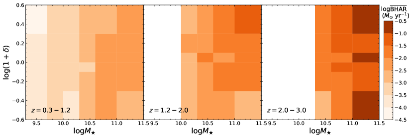
To probe the dependence on overdensity at different redshifts, we first bin sources into redshift ranges of , , and , respectively. We restrict our analyses to sources above the completeness limits, , 10, and 10.3, for redshift ranges of , , and , respectively (see Figs. 1 and 4). Applying these cuts is crucial, because incomplete samples could lead to biased values. For example, the at in the bin of would be strongly biased to , above which galaxies remain largely undetected (see Fig. 1 top). Therefore, such a value would not be representative of the entire redshift range of . Tab. 3 lists the sizes of these refined samples in different redshift ranges. Hereafter, this rule applies to all the analyses, unless otherwise stated. The fractions of our X-ray detected sources lying above the cuts are 96%, 90%, and 77% for redshift ranges of , , and , respectively (see Fig. 4). Therefore, we are still capturing most accretion power after applying the cuts. For each redshift bin, we further divide the sources into overdensity bins of , , , , , and . These bin boundaries (, , 0, 0.1, and 0.3) roughly correspond to , 30%, 50%, 70%, and 90% percentiles of the distribution of all objects.
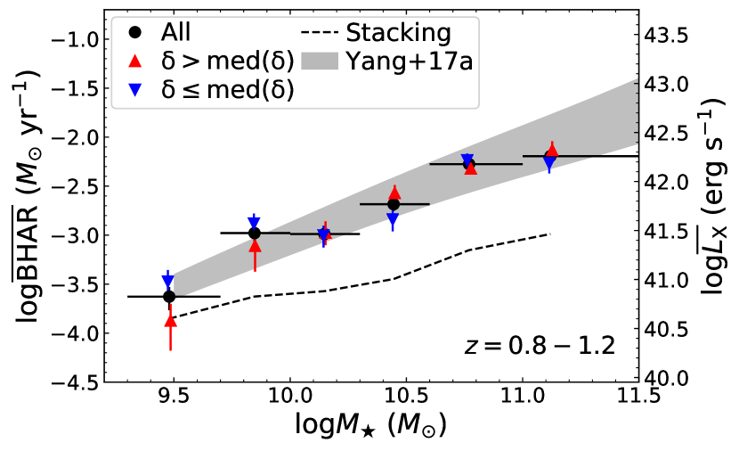
We calculate with the methods in §2.4.3 for all the bins and show the results in Fig. 6. tends to be slightly higher toward high overdensity (black points), likely due to the positive dependence between and overdensity and the intrinsic - correlation (see Fig. 4; e.g. Xue et al. 2010; Georgakakis et al. 2017; Yang et al. 2017, 2018; Aird et al. 2018). To show the dependence on , we divide each overdensity sample into high- and low- subsamples. In Fig. 6-left, the high- and low- subsamples have above and below the median of the overdensity sample, respectively; in Fig. 6-right, the high- and low- subsamples include sources with the highest 20% and the lowest 20% of the overdensity sample, respectively. In both the left and right panels, the high- subsamples have significantly higher than their corresponding low- subsamples, indicating the previously known strong - correlation. The differences between the high- and low- subsamples are generally larger in the right panels than in the corresponding left panels, as expected from the positive - correlation.
To investigate the potential -overdensity correlation for the controlled sample, we divide the sources into bins of , 9.7–10, 10–10.3, 10.3–10.6, 10.6–11, and 11–11.5 for each redshift range. The bin widths are dex and the limits at , 2.0, and 3.0 (§2.2) are chosen as the boundaries of the bins. We then split each sample into high-overdensity and low-overdensity subsamples in a similar way as in Fig. 6.
We calculate for all the samples and overdensity subsamples. The results are shown in Fig. 7 (left). The high-overdensity and low-overdensity subsamples do not appear to have significantly different , indicating that SMBH growth does not have a strong dependence on local environment at a given . Any small apparent differences between the high-overdensity and low-overdensity subsamples are likely just due to statistical fluctuations, as some blue points in Fig. 7 (left) are slightly above the corresponding red points while other blue points are below. The subsamples’ median uncertainty is 0.09 dex. Therefore, if the high-overdensity and low-overdensity subsamples had differing by dex systematically, the blue and red points would be significantly separated in Fig. 7 (left). In all redshift bins, rises toward the high regime. Yang et al. (2018) have modeled the - relations at different redshifts in detail, and our data points are consistent with their results (see Fig. 7). The contributed from stacking is generally dex lower than the total . Therefore, most X-ray emission is from the X-ray detected sources.
The two-subsample split (Fig. 7 left) guarantees that both subsamples have half the number of sources in each bin, and thus the uncertainties are relatively small (median uncertainty dex) for the subsamples. We also probe more extreme overdensity regimes by comparing of subsamples with the highest 20% of overdensities and the lowest 20% of overdensities (see Fig. 7 right). The high-overdensity and low-overdensity subsamples also have similar in general, although the uncertainties become larger (median uncertainty 0.13 dex) compared to those in Fig. 7 (left) due to reduced subsample sizes. In Fig. 7, there are 2 pairs of high-overdensity and low-overdensity points that are separated above a confidence level. These deviations are likely due to statistical fluctuations. There are a total of 26 pairs of points in Fig. 7 (i.e., 26 trials), and we expect to find such deviations (99% confidence level, calculated with a binomial distribution). Also, our detailed quantitative analyses in §3.1.2 do not find statistically significant -overdensity relation when is controlled.
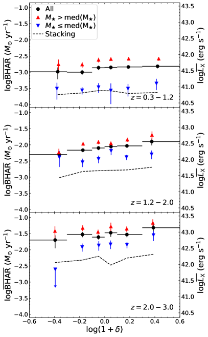
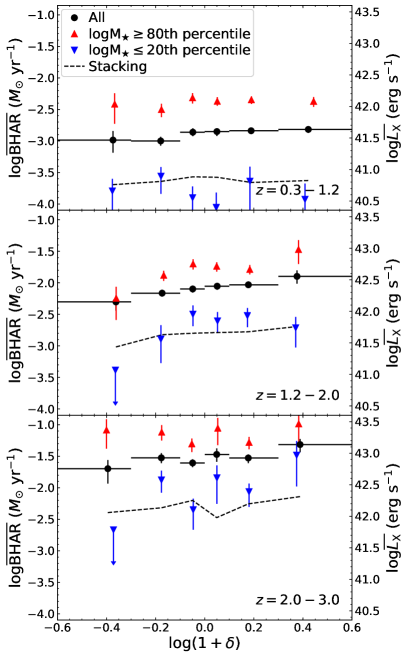
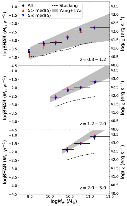
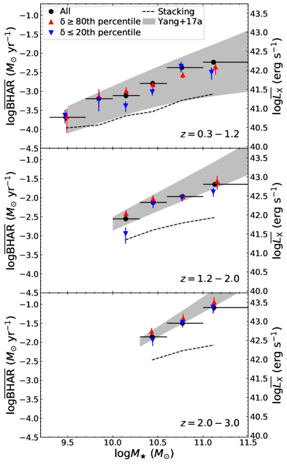
3.1.2 Partial Correlation Analyses
In §3.1.1, we qualitatively showed that the high-overdensity subsamples have similar as the corresponding low-overdensity subsamples when controlling for . This result indicates that SMBH growth, at a given , does not significantly depend on local environment. We further quantitatively verify this point via partial-correlation (PCOR) analysis (e.g. Johnson et al., 2002).
Following Yang et al. (2017), we utilize pcor.r in the r statistical package to perform PCOR analyses (Kim, 2015). We bin sources in the overdensity- plane and derive for each bin. The bin boundaries of overdensity and are the same as in §3.1.1. Fig. 8 shows the resulting on overdensity- grids. Similar to Yang et al. (2017), we input the , , and values into pcor.r, where the and are the medians in each bin. We study the -overdensity (-) correlation while controlling for the effects of (overdensity) via all three statistics available in pcor.r (Pearson, Spearman, and Kendall). The Pearson statistic assumes log-linear relations, while the Spearman and Kendall non-parametric statistics are rank-based and do not have such assumptions.
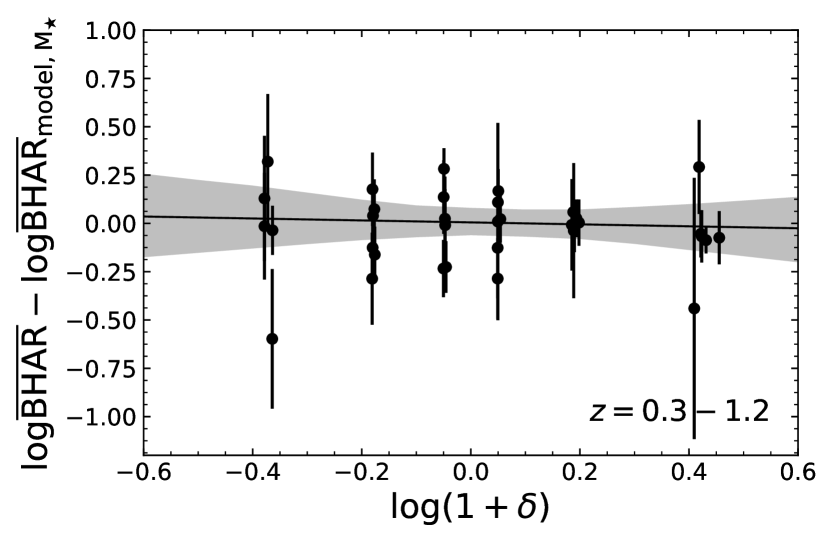
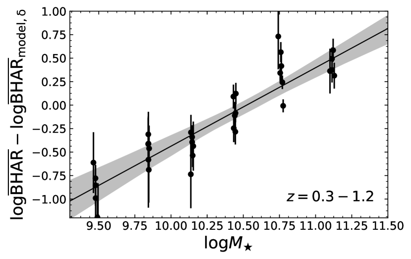
The results are listed in Tab. 3. The - correlation is statistically significant for all statistical techniques and across all redshift ranges. In contrast, the -overdensity correlation is not significant () under any statistic in any redshift range. To visualize the PCOR results, we perform a least- log-linear fit of the - (-overdensity) relation. We then fit the residual as a function of overdensity (). This procedure is similar to the Pearson statistic in PCOR analyses. The uncertainties of the best fit are estimated based on Markov chain Monte Carlo (MCMC) sampling with emcee (Foreman-Mackey et al., 2013). Fig. 9 displays the fitting results for . The best fit of the residual -overdensity relation is consistent with a flat model at a confidence level, while the residual - relation is steep. The conclusion also holds for the other two redshift ranges. In Fig. 9-bottom, the data points at tend to be above the fit. This perhaps indicates a log-linear model (assumed in the Pearson statistic) is not enough to describe fully the - relation, consistent with previous works (e.g. Georgakakis et al. 2017; Aird et al. 2018; Yang et al. 2018). The Spearman and Kendall statistics do not assume a log-linear model, and they lead to qualitatively similar results as the Pearson statistic (see Tab. 3). Also, we note that since there are a total of such 12 trials in Fig. 9 (considering both the top and bottom panels), it is not surprising that one such deviation happens by chance (see §3.1.1).
Therefore, we conclude that the significantly depends on but not overdensity. The conclusion is qualitatively supported by Figs. 1, 4, and 8. In Figs. 1 and 4, the X-ray detected sources preferentially appear in the high- regime but do not show much dependence on overdensity. In Fig. 4, X-ray sources have median overdensity values similar to those of all galaxies. In Fig. 8, the gradient is strong in the () direction but weak in the (overdensity) direction.
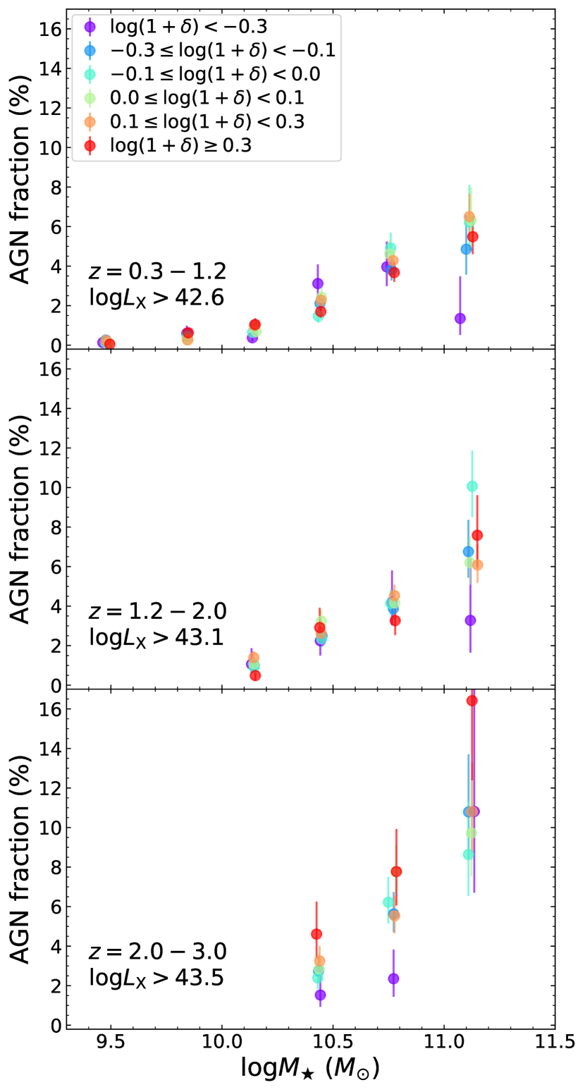
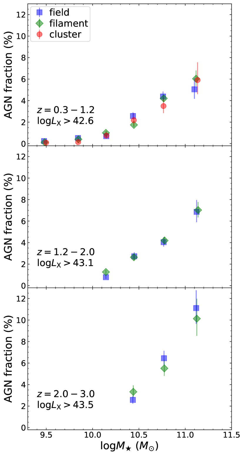
Our analyses above are based on the technique to assess SMBH growth. Another common technique in the literature is to consider AGN fractions above a given threshold (e.g. Silverman et al., 2009; Xue et al., 2010). Compared to our approach, the AGN-fraction approach is less informative and less physical, because it needs a pre-defined threshold which depends on X-ray survey sensitivity, and it does not consider X-ray emission from undetected sources. Also, unlike the approach, the AGN-fraction method weights low- and high- AGNs equally, as long as they are above the threshold, thereby sacrificing information. However, the AGN-fraction method still serves as a common alternative way to assess SMBH accretion (e.g. Lehmer et al. 2013; Martini et al. 2013). For a consistency check, we also present the AGN fractions in different bins for different local environments in Tab. 4 and Fig. 10. The AGN fractions are calculated as the fractions of X-ray detected sources above (), (), and (), respectively. For each redshift range, the threshold is chosen as the completeness limit at the redshift upper boundary (see Fig. 1). Due to the differences in thresholds, the AGN fractions (Tab. 4) at different redshift ranges are not directly comparable. The AGN-fraction errors are derived as binomial uncertainties using the astropy module “binom_conf_interval” (e.g. Cameron, 2011). From Tab. 6 and Fig. 10, at given and redshift, the AGN fractions are generally similar in different overdensity bins, consistent with our PCOR analyses. This consistency indicates that our conclusions are not affected by the X-ray stacking procedures (especially the masking of X-ray extended sources; see §2.4.2), since the AGN fractions are based on X-ray detected sources only. Also, the AGN fraction rises toward massive galaxies, as expected from the strong - relation (Fig. 7). In Fig. 10 (both top and middle panels), the lowest overdensity bin appears to have lower AGN fraction than other overdensity bins at . However, the differences are not significant at a 2 confidence level. Also, considering there are many (78) points in Fig. 10, it is natural that a few deviations happen considering the “number of trials” effect detailed in §3.1.1. Therefore, we consider the apparent differences are likely due to statistical fluctuations.
| (48,581 galaxies) | |||
| Relation | Pearson | Spearman | Kendall |
| -overdensity | 0.9 (0.1) | 0.2 (1.2) | 0.6 (0.6) |
| - | 10-48 (14.7) | 10-45 (14.1) | 10-10 (6.3) |
| (18,944 galaxies) | |||
| Relation | Pearson | Spearman | Kendall |
| -overdensity | 0.08 (1.7) | 0.4 (0.8) | 0.4 (0.8) |
| - | 10-33 (12.0) | 10-21 (9.5) | 10-7 (5.0) |
| (5,932 galaxies) | |||
| Relation | Pearson | Spearman | Kendall |
| -overdensity | 0.08 (1.8) | 0.1 (1.6) | 0.4 (0.9) |
| - | 10-19 (8.9) | 10-19 (9.0) | 10-5 (4.3) |
| () | |||||||
|---|---|---|---|---|---|---|---|
| 9.3–9.7 | 9.7–10.0 | 10.0–10.3 | 10.3–10.6 | 10.6–11.0 | 11.0–11.5 | ||
| All | |||||||
| () | |||||||
| – | – | 10.0–10.3 | 10.3–10.6 | 10.6–11.0 | 11.0–11.5 | ||
| – | – | ||||||
| – | – | ||||||
| – | – | ||||||
| – | – | ||||||
| – | – | ||||||
| – | – | ||||||
| All | – | – | |||||
| () | |||||||
| – | – | – | 10.3–10.6 | 10.6–11.0 | 11.0–11.5 | ||
| – | – | – | |||||
| – | – | – | |||||
| – | – | – | |||||
| – | – | – | |||||
| – | – | – | |||||
| – | – | – | |||||
| All | – | – | – | ||||
3.2 vs. Cosmic-Web Environment
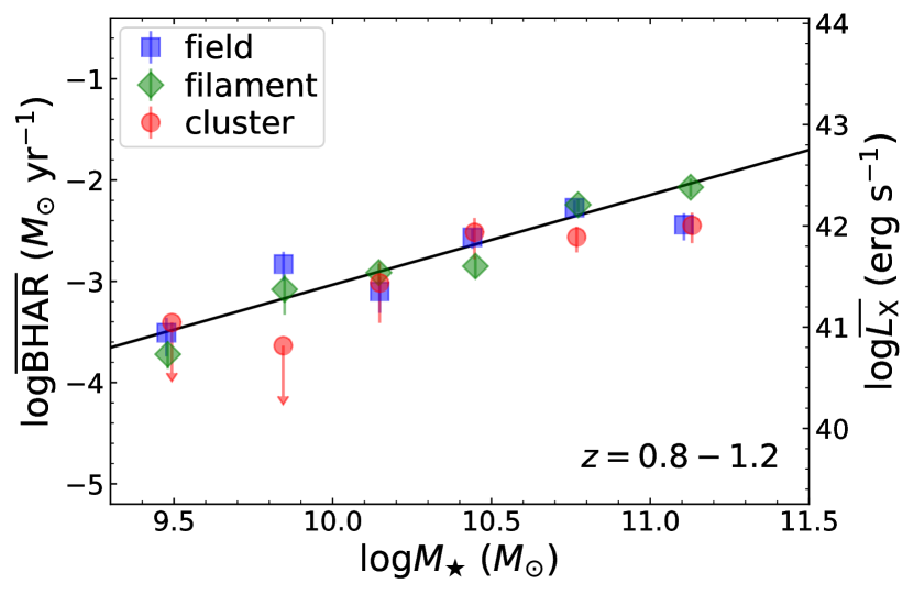
In §3.1, we show that the is not related to overdensity (on sub-Mpc scales) at given . In this section, we investigate the dependence of on cosmic-web environment ( Mpc scales). Following §3.1.1, we derive the for galaxies in field, filament, and cluster environments, respectively. The cosmic web describes global environment on Mpc scales (§2.3.2). The results are displayed in Fig. 11. The does not show a significant trend as a function of cosmic-web environment. For each environment bin, we further divide the sources into high- and low- subsamples, respectively, and calculate for each subsample. Similar to Fig. 6, the high- subsamples have significantly higher than the corresponding low- subsamples, consistent with the dominant - relation (§3.1).
We also bin our samples based on , and further divide each bin into subsamples for different parts of the cosmic web. We calculate for each subsample and show the results in Fig. 12. The values are not systematically different for different cosmic-web environments.
Now we test the dependence on cosmic-web environment quantitatively. Unlike in §3.1.2, we do not perform a PCOR analysis, because the cosmic-web environment (field, filament, and cluster) is not a continuous quantity. Instead, we employ another statistical analysis based on the Akaike information criterion (AIC; Akaike 1974). The AIC is designed for model selection and defined as , where is the fitting statistic ( for least squares fitting) and is the number of free parameters in the model. If one model has an AIC value much smaller than another model (), then the former is considered superior to the latter (see, e.g. §2.6 of Burnham & Anderson 2002). In our analyses, we choose , corresponding to a 3 confidence level under the situation where the model parameter uncertainties are Gaussian (e.g. Murtaugh 2014).
We apply the AIC technique to our data points in Fig. 12. For each redshift range, we perform a least- fit to all the data points with a log-linear model, , where and are free model parameters.444The single upper limit point in Fig. 12 is not used in the fitting. We calculate the AIC value (AIC1) for this fitting. The best-fit models are displayed in Fig. 12. We then create a set of three independent log-linear models, i.e., , , and , to fit the data.555For , we only create the field and filament models, as we do not assign cluster environment (see §2.3.2). As the subscripts indicate, each model is used to fit the data points of the corresponding cosmic-web environment in Fig. 12. We derive the AIC value (AIC2) for this multi-model fitting. If , then the - relations might be different for different cosmic-web environments. The resulting AIC values are listed in Tab. 5. For all three redshift ranges, the values are above . Therefore, the differences among the - relations for different cosmic-web environments are not statistically significant. However, the non-detection of a -environment correlation might be, in principle, due to the limited sensitivity of our data. Martini et al. (2009) found that the AGN fraction in rich clusters is dex below that in the field at . A natural question is whether our data are sensitive enough to detect such differences, i.e., drops by 0.7 dex from the field to cluster environments. To answer this question, we perform a test. For our bin, we systematically shift our cluster (field) by dex ( dex) and re-calculate . We find , much lower than our threshold (). Therefore, if our dropped by 0.7 dex from the field to cluster environments, we would definitely detect the environmental dependence of . In fact, we find that our data are sensitive at a level to a dex difference of from the field to cluster environments at . This difference between our work and Martini et al. (2009) might be due to the lack of rich clusters in our sample (see §4.1 for more discussion).
In Fig. 13, we also compare for cluster and field environments at . Here, we limit the cluster (field) galaxies to those with the highest (lowest) 20% overdensity in each bin.666Here, we do not limit cluster galaxies to those also identified by George et al. (2011), because this would lead to too few sources (only AGNs) for our analyses, as the cluster-member catalog in George et al. (2011) is not complete (see §2.3.2). In this way, we probe the most-extreme environments. We perform AIC analyses and obtain , above the threshold (). Therefore, the - relations for these two extreme environments are also not statistically different. At higher redshift, we have also performed similar analyses for filament vs. field environments and reached the same conclusion.
As in §3.1.2, we also calculate AGN fractions for different cosmic-web environments for a consistency check. The results are presented in Tab. 6 and Fig. 14. The AGN fractions are generally similar for different cosmic-web environments when controlling for , consistent with our AIC analyses. Our AGN fractions for are at . This range is consistent with the results of Silverman et al. (2009, see their Tab. 2), who found an AGN fraction of for at , independent of environment. Our AGN fractions for at are , similar to that derived for SDSS galaxies of similar at (Haggard et al., 2010).
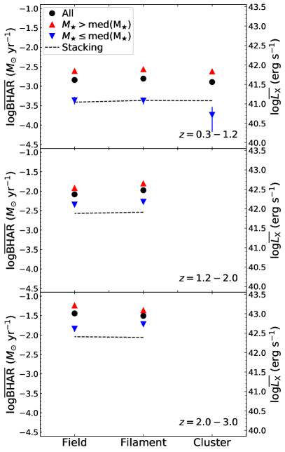
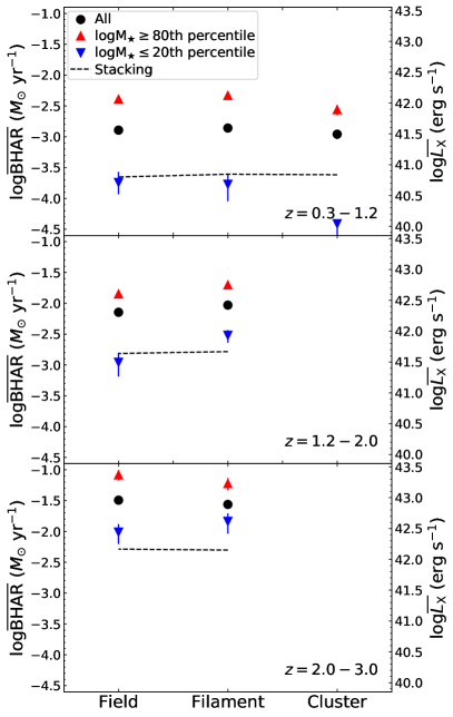
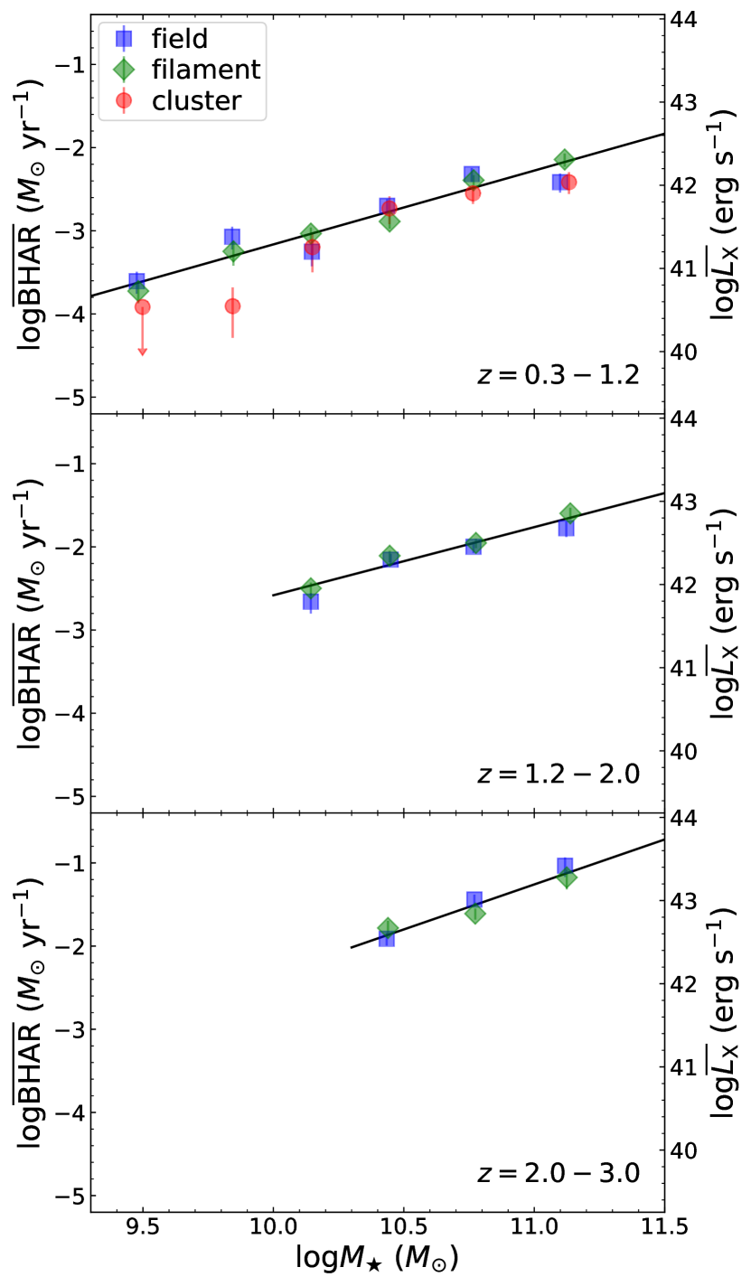
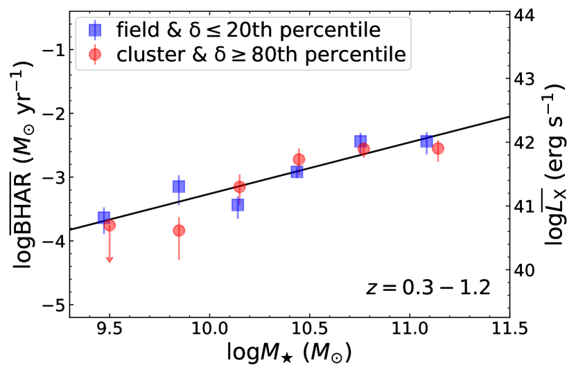
| Redshift | AIC1 | AIC2 | |
|---|---|---|---|
| 0.3–1.2 | 32.48 | 33.35 | |
| 1.2–2.0 | 12.34 | 14.38 | |
| 2.0–3.0 | 9.82 | 9.75 |
| () | |||||||
|---|---|---|---|---|---|---|---|
| 9.3–9.7 | 9.7–10.0 | 10.0–10.3 | 10.3–10.6 | 10.6–11.0 | 11.0–11.5 | ||
| Field | |||||||
| Filament | |||||||
| Cluster | |||||||
| All | |||||||
| () | |||||||
| – | – | 10.0–10.3 | 10.3–10.6 | 10.6–11.0 | 11.0–11.5 | ||
| Field | – | – | |||||
| Filament | – | – | |||||
| All | – | – | |||||
| () | |||||||
| – | – | – | 10.3–10.6 | 10.6–11.0 | 11.0–11.5 | ||
| Field | – | – | – | ||||
| Filament | – | – | – | ||||
| All | – | – | – | ||||
3.3 Tests in Narrower Redshift Bins
Our analyses above adopt relatively wide redshift bins, i.e., , 1.2–2.0, and 2.0–3.0, to retain relatively large sample size in each bin. Considering that both galaxy and AGN properties as well as cosmic environment evolve with redshift, the -environment relation might also have redshift dependence. To test for possible redshift dependence, we repeat our analyses in §3.1 and §3.2 using narrower redshift bins, i.e., , 0.8–1.2, 1.2–1.6, 1.6–2.0, 2.0–2.5, and 2.5–3.0. This procedure reduces the sample size in each bin and thus increases the uncertainties on in general. In the new analyses with narrower redshift bins, we still do not find any significant dependence on either overdensity or cosmic-web environment, consistent with the results in §3.1 and §3.2. Fig. 15 shows some example figures for , and the figures for other narrower redshift bins are qualitatively similar. Therefore, our main conclusions are unlikely to be affected by our choice of relatively wide redshift bins.
4 Discussion
We discuss the physical implications of our results in §4.1. We compare our results with previous observations of BHAR-environment relations in §4.2.
4.1 Physical Implications
Our results indicate that SMBH accretion is fundamentally related to . At a given , our does not show significant dependence on host-galaxy environment. Since galaxy environment is largely determined by dark matter, which generally dominates the gravitational field on subMpc scales, our conclusions suggest SMBH growth is primarily related to baryons rather than dark matter (e.g. Kormendy & Ho, 2013; Yang et al., 2018). The broad physical picture is likely that dark-matter density fluctuations lead to the formation of halos, allowing baryons to condense into the halo centers and form galaxies. The galaxies feed their SMBHs with cold gas via baryonic physics, e.g. disk instabilities and galaxy bars (e.g. Alexander & Hickox 2012 and references therein). This scenario indicates that, in future studies of SMBH-galaxy coevolution, it is critical to focus on relations between BHAR and host-galaxy intrinsic properties (e.g. , SFR, and morphology) rather than the environment. Small but deep surveys such as the Chandra Deep Fields (e.g. Xue et al. 2016; Luo et al. 2017) and CANDELS (Grogin et al. 2011; Koekemoer et al. 2011) are ideal for studying SMBH-galaxy coevolution.
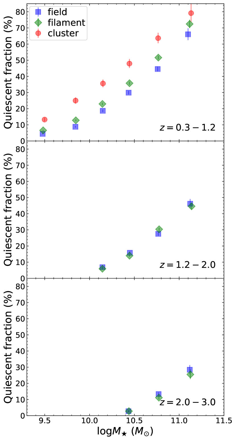
It is well established that environment affects galaxy evolution. At a given and at , the quiescent-galaxy fraction (as defined in §2.2) rises toward high-density regions, and this effect is often termed “environmental quenching” (e.g. Peng et al. 2010; Scoville et al. 2013; Darvish et al. 2015, 2016; Darvish et al. 2017; Laigle et al. 2018). Fig. 16 shows the quiescent-galaxy fraction in our sample as a function of for different cosmic-web environments (see §2.2 for star-forming/quiescent classifications). At and a given , the quiescent galaxy fraction significantly rises from the field to cluster environments; at higher redshifts this environmental dependence seems to disappear. Therefore, environmental quenching at is significantly observed in our sample. For a given cosmic-web environment, the quiescent-galaxy fraction also rises toward high at all redshifts. This dependence is expected from previous studies (e.g. Brammer et al., 2011; Davidzon et al., 2017).
In contrast, our does not show a significant dependence on environment, if is controlled (see §3). These different behaviors of SMBH accretion and star formation suggest that SMBH and galaxy stellar-mass growth are not strongly coupled in general (e.g. Yang et al. 2017, 2018), although we cannot rule out a weak secondary -SFR relation (see §4.2). The potential physical mechanisms responsible for environmental quenching such as tidal interaction and ram-pressure stripping (§1) might only have limited effects on SMBH accretion.
Since galaxy evolution has significant dependence on environment at low redshift (), the host-galaxy types of AGNs might also depend on environment. In Tab. 7, we list the quiescent-galaxy fractions for AGNs (as defined in §3.1.2) in different cosmic-web environments. At , the quiescent-galaxy fraction of AGN hosts appears to rise from the field to clusters, similar to the trend for normal galaxies (see Fig. 16). At higher redshift, if anything, the trend seems to be the opposite going from the field to filament environments. However, these trends are not statistically significant at a 3 confidence level due to our limited AGN sample size. Future work with much larger AGN samples can determine these trends more accurately.
| Redshift | Field | Filament | Cluster | All |
|---|---|---|---|---|
| – | ||||
| – |
4.2 Previous Works on BHAR vs. Environment
Based on sources at , observations have found that cluster () and field environments have similar X-ray AGN fractions among massive galaxies, consistent with our results (e.g. Georgakakis et al. 2008; Silverman et al. 2009; Koulouridis et al. 2014). However, these analyses are often restricted to low-redshift relatively bright galaxies. Thanks to the reliable photo- measurements and our improved methodology for assessing SMBH accretion, our work is able to investigate -environment relations for all galaxies above the completeness limits up to . Importantly, our study covers where cosmic AGN activity peaks.
Some studies find that, at , the X-ray AGN fractions in rich clusters () are generally lower than those in the field (e.g. Martini et al. 2009; Ehlert et al. 2014). Due to the lack of excellent multiwavelength coverage for calculation, these studies often adopt a simple -band magnitude cut to approximate an cut of the galaxy population (e.g. Cappellari 2016). However, we note that consensus has not been widely reached on whether rich clusters have lower AGN fractions than the field. For example, Haggard et al. (2010) found that rich clusters and the field have similar AGN fractions at , when the same magnitude and cuts are applied to the cluster and field populations. If AGN activity is indeed suppressed in rich clusters at a given , the physical reason might be different galaxy types in cluster and field environments. Rich clusters, especially in their central regions, are dominated by the quiescent galaxy population, which tends to have lower AGN fractions than the star-forming population at a given (e.g. Wang et al. 2017; Aird et al. 2018; Yang et al. 2018). We cannot study such rich clusters in our work, because they are rare and generally absent in COSMOS, where the clusters typically have (e.g. Knobel et al. 2009; George et al. 2011). However, only a small fraction of the galaxy population () lives in rare rich clusters with (e.g. Tab. 1 of Bahcall, 1999). Our work covers a large comoving volume ( Mpc3 for each redshift bin; §2.1), and thus we probe the main range of cosmic environments in the overall Universe with . We do not find significant -environment relations when controlling for , even at the extremes of the environments we sample (e.g. Figs. 7 and 13). Therefore, we conclude that, for the overall galaxy population, generally does not depend on cosmic environment once is controlled, although this conclusion might not hold for galaxies living in rare rich clusters.
At high redshift (), observations suggest that some massive protoclusters might have elevated AGN activity (see §1; but also see Macuga et al. 2018). For example, SSA 22 is a prominent protocluster at , and it is likely a progenitor of local rich clusters with (e.g. Steidel et al., 1998). Lehmer et al. (2009) estimated that its X-ray AGN fraction is among Lyman Break Galaxies (LBGs) and Ly Emitters (LAEs), considerably higher than the AGN fraction () among LBGs and LAEs in the field at similar redshifts. However, the LBGs and LAEs in SSA 22 might have different compared to the LBGs and LAEs in the field, and the difference in could drive the apparent differences in AGN fraction (see Tab. 6). Also, the SSA 22 AGN sample size is limited () and suffers from significant statistical uncertainty. SSA 22 has galaxies in its central region of Mpc2 (e.g. Topping et al., 2016), translating to an overdensity value of (§2.3.1). We do not have such prominent structures in our sample at (Fig. 1) and thus cannot probe their AGN activity using COSMOS. Note that the estimated overdensity value of SSA 22 is for high redshifts (). It is not directly comparable to our structures at low redshift, since the normalization factors are different at different redshifts (see Eq. 1).
AGN-clustering studies also make use of source spatial distributions to probe SMBH-galaxy coevolution. Early observations found that X-ray AGNs and normal galaxies appear to have different clustering properties (especially on Mpc comoving scales), suggesting different environmental effects for central vs. satellite galaxies (e.g. Hickox et al. 2009; Miyaji et al. 2011; Allevato et al. 2012). However, galaxy properties (especially ) were not carefully controlled among these studies. Considering the strong - correlation (e.g. Yang et al., 2017, 2018) and the well-established relation between galaxy clustering and (e.g. Coil et al., 2006, 2017), it is critical to match in AGN vs. galaxy clustering analyses. More recent observations show that the clustering properties of AGNs and galaxies are similar over a wide range of comoving scale ( Mpc ) when is carefully matched, indicating that (rather than a central/satellite effect) mainly drives the observed clustering properties of AGNs (e.g. Georgakakis et al. 2014; Powell et al. 2018). Also, our analyses do not support different environmental effects for central vs. satellite galaxies, although we do not perform a central/satellite classification (§2.3). If, for example, environment only affects AGN activity in central galaxies, we would witness an increasingly strong -environment relation in more massive galaxies which have a higher chance of being central (e.g. Reddick et al. 2013). However, we do not find any significant -environment correlation over a wide range of stellar mass (; §3). Clustering analyses infer that AGNs typically have (e.g. Allevato et al. 2011, 2014, 2016; Richardson et al. 2013). This is as expected, since low-mass halos () only host low-mass galaxies with weak and high-mass halos () are rare.
5 Summary and Future Work
We have studied the dependence on and environment in redshift bins of , , and , based on sources in the COSMOS field. Our main procedures and results are summarized below:
- 1.
-
2.
We have derived for different samples, considering both X-ray detected and undetected sources (§2.4). For X-ray detected sources, we adopt, in order of priority, hard-band, full-band, and soft-band fluxes, in our calculations (§2.4.1). This choice is to minimize the effects of X-ray obscuration. We include the X-ray emission from X-ray undetected sources via stacking (§2.4.2).
-
3.
We do not find a statistically significant dependence on overdensity or cosmic-web environment ( Mpc) for controlled samples (§3). Instead, is always strongly related to , regardless of environment. These results suggest that might be primarily related to the host galaxies rather than cosmic environment on scales of Mpc, which is determined by dark matter (§4.1). Thanks to the large comoving volume sampled ( Mpc3 for each redshift bin), we can probe the main range of cosmic environments in the overall Universe (§4.2). Therefore, we conclude that, for the overall galaxy population, generally does not depend on cosmic environment once is controlled, although this conclusion might not hold for the of galaxies living in rare rich clusters with .
-
4.
In contrast to SMBH accretion, star formation activity significantly depends on environment at (§4.1). For our sample, the quiescent-galaxy fraction rises from the field to cluster environment for -controlled samples at , consistent with previous observations. The different behaviors of SMBH accretion and star formation suggest that SMBH and galaxy growth are not strongly coupled in general. Environment-related mechanisms such as tidal interaction and ram-pressure stripping that could shape galaxy evolution do not appear to strongly affect SMBH growth.
Future work can probe the dependence on environment for larger physical scales ( Mpc). Since COSMOS alone cannot sample the full range of cosmic environments on these scales (e.g. Meneux et al. 2009; Skibba et al. 2014), these studies will need several COSMOS-like fields, e.g. XMM-LSS (Chen et al., 2018), Wide-CDF-S, and ELAIS-S1, or much larger fields such as Stripe 82 (LaMassa et al., 2013) and XMM-XXL (Pierre et al., 2016). Such larger fields can also be used to probe SMBH growth in rare rich clusters/protoclusters (see §4.2) while controlling for host-galaxy properties, especially . In addition, future work may study in galaxy close pairs on kpc scales (e.g. Mundy et al., 2017).
The upcoming eROSITA all-sky X-ray survey will yield a sample of AGNs at (e.g. Merloni et al. 2012), allowing studies of -environment relations at low-to-moderate redshift with overwhelming source statistics. In this work, we do not find significant environmental dependence of average BHAR. It is still possible that the full distribution of BHAR depends on environment, although this would require “finely tuned” BHAR distributions in different environments to maintain constant . A full characterization of the BHAR distribution as a function of , environment, and redshift (e.g. Georgakakis et al. 2017; Aird et al. 2018; Yang et al. 2018) requires future X-ray observatories like Athena and Lynx, which are necessary to sample the faint end of the BHAR distribution in COSMOS-like (or larger) fields (e.g. Georgakakis 2018).
With the advance of environment-measurement methodology, new environmental metrics other than overdensity (and the consequent field/filament/cluster classification) may be developed. Future work can study the dependence on these new environmental metrics (e.g. mass density instead of number density as used in this work). Future spectroscopic observations with Extremely Large Telescopes (ELTs) should improve the spec- completeness for COSMOS and other fields by a large factor, allowing environmental measurements with superior accuracy (e.g. reducing the projection distance from Mpc to Mpc; Appendix A). Based on such new spec- data, studies can revisit the -environment- connection, even for central/satellite galaxies separately.
Acknowledgements
We thank the referee for helpful feedback that improved this work. We thank Francesca Civano, Clotilde Laigle, and Mara Salvato for providing relevant data. We thank Robin Ciardullo, Antonis Georgakakis, Ryan Hickox, Donghui Jeong, Paul Martini, Qingling Ni, John Silverman, Michael Strauss, and Rosemary Wyse for helpful discussions. G.Y., W.N.B., C.T.C., and F.V. acknowledge support from Chandra X-ray Center grants GO4-15130A and AR8-19016X, NASA grant NNX17AF07G, and the NASA Astrophysics Data Analysis Program (ADAP). B.D. acknowledges financial support from NASA through the ADAP, grant number NNX12AE20G, and the National Science Foundation, grant number 1716907. D.M.A. acknowledges the Science and Technology Facilities Council (STFC) through grant ST/P000541/1. F.E.B. acknowledges support from CONICYT-Chile (Basal-CATA PFB-06/2007, FONDO ALMA 31160033) and the Ministry of Economy, Development, and Tourism’s Millennium Science Initiative through grant IC120009, awarded to The Millennium Institute of Astrophysics, MAS.
References
- Aird et al. (2017) Aird J., Coil A. L., Georgakakis A., 2017, MNRAS, 465, 3390
- Aird et al. (2018) Aird J., Coil A. L., Georgakakis A., 2018, MNRAS, 474, 1225
- Akaike (1974) Akaike H., 1974, IEEE transactions on automatic control, 19, 716
- Alexander & Hickox (2012) Alexander D. M., Hickox R. C., 2012, New Astronomy Reviews, 56, 93
- Alexander et al. (2016) Alexander D. M., et al., 2016, MNRAS, 461, 2944
- Allevato et al. (2011) Allevato V., et al., 2011, ApJ, 736, 99
- Allevato et al. (2012) Allevato V., et al., 2012, ApJ, 758, 47
- Allevato et al. (2014) Allevato V., et al., 2014, ApJ, 796, 4
- Allevato et al. (2016) Allevato V., et al., 2016, ApJ, 832, 70
- Aragón-Calvo et al. (2007) Aragón-Calvo M. A., Jones B. J. T., van de Weygaert R., van der Hulst J. M., 2007, A&A, 474, 315
- Aragón-Calvo et al. (2010) Aragón-Calvo M. A., van de Weygaert R., Jones B. J. T., 2010, MNRAS, 408, 2163
- Astropy Collaboration et al. (2013) Astropy Collaboration et al., 2013, A&A, 558, A33
- Astropy Collaboration et al. (2018) Astropy Collaboration et al., 2018, preprint, (arXiv:1801.02634)
- Bañados et al. (2013) Bañados E., Venemans B., Walter F., Kurk J., Overzier R., Ouchi M., 2013, ApJ, 773, 178
- Bahcall (1999) Bahcall N. A., 1999, Formation of Structure in the Universe, 4, 135
- Balmaverde et al. (2017) Balmaverde B., et al., 2017, A&A, 606, A23
- Balogh et al. (2004) Balogh M., et al., 2004, MNRAS, 348, 1355
- Brammer et al. (2011) Brammer G. B., et al., 2011, ApJ, 739, 24
- Brandt & Alexander (2015) Brandt W. N., Alexander D. M., 2015, A&ARv, 23, 1
- Burnham & Anderson (2002) Burnham K., Anderson D., 2002, Model selection and multimodel inference: a practical information-theoretic approach, 2, 49
- Calzetti et al. (2000) Calzetti D., Armus L., Bohlin R. C., Kinney A. L., Koornneef J., Storchi-Bergmann T., 2000, ApJ, 533, 682
- Cameron (2011) Cameron E., 2011, Publ. Astron. Soc. Australia, 28, 128
- Cappellari (2016) Cappellari M., 2016, ARA&A, 54, 597
- Cautun et al. (2014) Cautun M., Frenk C. S., van de Weygaert R., Hellwing W. A., Jones B. J. T., 2014, MNRAS, 445, 2049
- Chabrier (2003) Chabrier G., 2003, ApJ, 586, L133
- Chen et al. (2013) Chen C.-T. J., et al., 2013, ApJ, 773, 3
- Chen et al. (2018) Chen C.-T. J., et al., 2018, MNRAS,
- Ciesla et al. (2015) Ciesla L., et al., 2015, A&A, 576, A10
- Civano et al. (2016) Civano F., et al., 2016, ApJ, 819, 62
- Coil et al. (2006) Coil A. L., Newman J. A., Cooper M. C., Davis M., Faber S. M., Koo D. C., Willmer C. N. A., 2006, ApJ, 644, 671
- Coil et al. (2017) Coil A. L., Mendez A. J., Eisenstein D. J., Moustakas J., 2017, ApJ, 838, 87
- Conselice (2014) Conselice C. J., 2014, ARA&A, 52, 291
- Cooper et al. (2006) Cooper M. C., et al., 2006, MNRAS, 370, 198
- Darvish et al. (2014) Darvish B., Sobral D., Mobasher B., Scoville N. Z., Best P., Sales L. V., Smail I., 2014, ApJ, 796, 51
- Darvish et al. (2015) Darvish B., Mobasher B., Sobral D., Scoville N., Aragon-Calvo M., 2015, ApJ, 805, 121
- Darvish et al. (2016) Darvish B., Mobasher B., Sobral D., Rettura A., Scoville N., Faisst A., Capak P., 2016, ApJ, 825, 113
- Darvish et al. (2017) Darvish B., Mobasher B., Martin D. C., Sobral D., Scoville N., Stroe A., Hemmati S., Kartaltepe J., 2017, ApJ, 837, 16
- Davidzon et al. (2017) Davidzon I., et al., 2017, preprint, (arXiv:1701.02734)
- Davis & Laor (2011) Davis S. W., Laor A., 2011, ApJ, 728, 98
- De Lucia et al. (2006) De Lucia G., Springel V., White S. D. M., Croton D., Kauffmann G., 2006, MNRAS, 366, 499
- Dekel et al. (2009) Dekel A., et al., 2009, Nature, 457, 451
- Delvecchio et al. (2017) Delvecchio I., et al., 2017, A&A, 602, A3
- Desjacques et al. (2016) Desjacques V., Jeong D., Schmidt F., 2016, preprint, (arXiv:1611.09787)
- Digby-North et al. (2010) Digby-North J. A., et al., 2010, MNRAS, 407, 846
- Draine & Li (2007) Draine B. T., Li A., 2007, ApJ, 657, 810
- Dressler (1980) Dressler A., 1980, ApJ, 236, 351
- Ebeling et al. (2014) Ebeling H., Stephenson L. N., Edge A. C., 2014, ApJ, 781, L40
- Ehlert et al. (2014) Ehlert S., et al., 2014, MNRAS, 437, 1942
- Elbaz et al. (2007) Elbaz D., et al., 2007, A&A, 468, 33
- Farouki & Shapiro (1981) Farouki R., Shapiro S. L., 1981, ApJ, 243, 32
- Finoguenov et al. (2007) Finoguenov A., et al., 2007, ApJS, 172, 182
- Foreman-Mackey et al. (2013) Foreman-Mackey D., Hogg D. W., Lang D., Goodman J., 2013, PASP, 125, 306
- Fragos et al. (2013) Fragos T., et al., 2013, ApJ, 764, 41
- Georgakakis (2018) Georgakakis A., 2018, Athena Nuggets, 24
- Georgakakis et al. (2008) Georgakakis A., Gerke B. F., Nandra K., Laird E. S., Coil A. L., Cooper M. C., Newman J. A., 2008, MNRAS, 391, 183
- Georgakakis et al. (2014) Georgakakis A., et al., 2014, MNRAS, 443, 3327
- Georgakakis et al. (2017) Georgakakis A., Aird J., Schulze A., Dwelly T., Salvato M., Nandra K., Merloni A., Schneider D. P., 2017, MNRAS, 471, 1976
- George et al. (2011) George M. R., et al., 2011, ApJ, 742, 125
- Grogin et al. (2011) Grogin N. A., et al., 2011, ApJS, 197, 35
- Gunn & Gott (1972) Gunn J. E., Gott III J. R., 1972, ApJ, 176, 1
- Haggard et al. (2010) Haggard D., Green P. J., Anderson S. F., Constantin A., Aldcroft T. L., Kim D.-W., Barkhouse W. A., 2010, ApJ, 723, 1447
- Hasinger et al. (2018) Hasinger G., et al., 2018, ApJ, 858, 77
- Hickox et al. (2009) Hickox R. C., et al., 2009, ApJ, 696, 891
- Hickox et al. (2014) Hickox R. C., Mullaney J. R., Alexander D. M., Chen C.-T. J., Civano F. M., Goulding A. D., Hainline K. N., 2014, ApJ, 782, 9
- Hopkins et al. (2006) Hopkins P. F., Hernquist L., Cox T. J., Di Matteo T., Robertson B., Springel V., 2006, ApJS, 163, 1
- Hopkins et al. (2007) Hopkins P. F., Richards G. T., Hernquist L., 2007, ApJ, 654, 731
- Hsu et al. (2014) Hsu L.-T., et al., 2014, ApJ, 796, 60
- Ilbert et al. (2009) Ilbert O., et al., 2009, ApJ, 690, 1236
- Ilbert et al. (2010) Ilbert O., et al., 2010, ApJ, 709, 644
- Ilbert et al. (2013) Ilbert O., et al., 2013, A&A, 556, A55
- Johnson et al. (2002) Johnson R. A., Wichern D. W., et al., 2002, Applied multivariate statistical analysis. Vol. 5, Prentice Hall Upper Saddle River, NJ
- Karhunen et al. (2014) Karhunen K., Kotilainen J. K., Falomo R., Bettoni D., 2014, MNRAS, 441, 1802
- Kauffmann et al. (2004) Kauffmann G., White S. D. M., Heckman T. M., Ménard B., Brinchmann J., Charlot S., Tremonti C., Brinkmann J., 2004, MNRAS, 353, 713
- Kereš et al. (2005) Kereš D., Katz N., Weinberg D. H., Davé R., 2005, MNRAS, 363, 2
- Kim (2015) Kim S., 2015, Communications for statistical applications and methods, 22, 665
- King & Pounds (2015) King A., Pounds K., 2015, ARA&A, 53, 115
- Knobel et al. (2009) Knobel C., et al., 2009, ApJ, 697, 1842
- Knobel et al. (2012) Knobel C., et al., 2012, ApJ, 753, 121
- Koekemoer et al. (2011) Koekemoer A. M., et al., 2011, ApJS, 197, 36
- Kormendy & Ho (2013) Kormendy J., Ho L. C., 2013, ARA&A, 51, 511
- Koulouridis et al. (2014) Koulouridis E., et al., 2014, A&A, 567, A83
- Kravtsov & Borgani (2012) Kravtsov A. V., Borgani S., 2012, ARA&A, 50, 353
- LaMassa et al. (2013) LaMassa S. M., et al., 2013, MNRAS, 436, 3581
- Laigle et al. (2016) Laigle C., et al., 2016, ApJS, 224, 24
- Laigle et al. (2018) Laigle C., et al., 2018, MNRAS, 474, 5437
- Lehmer et al. (2009) Lehmer B. D., et al., 2009, ApJ, 691, 687
- Lehmer et al. (2013) Lehmer B. D., et al., 2013, ApJ, 765, 87
- Lehmer et al. (2016) Lehmer B. D., et al., 2016, ApJ, 825, 7
- Li et al. (2006) Li C., Kauffmann G., Wang L., White S. D. M., Heckman T. M., Jing Y. P., 2006, MNRAS, 373, 457
- Lietzen et al. (2009) Lietzen H., et al., 2009, A&A, 501, 145
- Lilly et al. (2009) Lilly S. J., et al., 2009, ApJS, 184, 218
- Lin et al. (2010) Lin L., et al., 2010, ApJ, 718, 1158
- Liu et al. (2017) Liu T., et al., 2017, ApJS, 232, 8
- Luo et al. (2010) Luo B., et al., 2010, ApJS, 187, 560
- Luo et al. (2017) Luo B., et al., 2017, ApJS, 228, 2
- Lusso et al. (2012) Lusso E., et al., 2012, MNRAS, 425, 623
- Macuga et al. (2018) Macuga M., et al., 2018, preprint, (arXiv:1805.06569)
- Madau & Dickinson (2014) Madau P., Dickinson M., 2014, ARA&A, 52, 415
- Malavasi et al. (2016) Malavasi N., Pozzetti L., Cucciati O., Bardelli S., Cimatti A., 2016, A&A, 585, A116
- Marchesi et al. (2016a) Marchesi S., et al., 2016a, ApJ, 817, 34
- Marchesi et al. (2016b) Marchesi S., et al., 2016b, ApJ, 830, 100
- Marconi et al. (2004) Marconi A., Risaliti G., Gilli R., Hunt L. K., Maiolino R., Salvati M., 2004, MNRAS, 351, 169
- Martini & Schneider (2003) Martini P., Schneider D. P., 2003, ApJ, 597, L109
- Martini et al. (2009) Martini P., Sivakoff G. R., Mulchaey J. S., 2009, ApJ, 701, 66
- Martini et al. (2013) Martini P., et al., 2013, ApJ, 768, 1
- McCracken et al. (2012) McCracken H. J., et al., 2012, A&A, 544, A156
- Meneux et al. (2009) Meneux B., et al., 2009, A&A, 505, 463
- Merloni et al. (2012) Merloni A., et al., 2012, preprint, (arXiv:1209.3114)
- Miyaji et al. (2011) Miyaji T., Krumpe M., Coil A. L., Aceves H., 2011, ApJ, 726, 83
- Moore et al. (1998) Moore B., Lake G., Katz N., 1998, ApJ, 495, 139
- Mundy et al. (2017) Mundy C. J., Conselice C. J., Duncan K. J., Almaini O., Häußler B., Hartley W. G., 2017, MNRAS, 470, 3507
- Murtaugh (2014) Murtaugh P. A., 2014, Ecology, 95, 611
- Noll et al. (2009) Noll S., Burgarella D., Giovannoli E., Buat V., Marcillac D., Muñoz-Mateos J. C., 2009, A&A, 507, 1793
- Novak et al. (2011) Novak G. S., Ostriker J. P., Ciotti L., 2011, ApJ, 737, 26
- Overzier (2016) Overzier R. A., 2016, A&ARv, 24, 14
- Peng et al. (2010) Peng Y.-j., et al., 2010, ApJ, 721, 193
- Pierre et al. (2016) Pierre M., et al., 2016, A&A, 592, A1
- Poggianti et al. (2016) Poggianti B. M., et al., 2016, AJ, 151, 78
- Poggianti et al. (2017) Poggianti B. M., et al., 2017, Nature, 548, 304
- Powell et al. (2018) Powell M. C., et al., 2018, ApJ, 858, 110
- Reddick et al. (2013) Reddick R. M., Wechsler R. H., Tinker J. L., Behroozi P. S., 2013, ApJ, 771, 30
- Richardson et al. (2013) Richardson J., Chatterjee S., Zheng Z., Myers A. D., Hickox R., 2013, ApJ, 774, 143
- Sartori et al. (2018) Sartori L. F., Schawinski K., Trakhtenbrot B., Caplar N., Treister E., Koss M. J., Megan Urry C., Zhang C., 2018, MNRAS,
- Scoville et al. (2007) Scoville N., et al., 2007, ApJS, 172, 150
- Scoville et al. (2013) Scoville N., et al., 2013, ApJS, 206, 3
- Serber et al. (2006) Serber W., Bahcall N., Ménard B., Richards G., 2006, ApJ, 643, 68
- Serra et al. (2011) Serra P., Amblard A., Temi P., Burgarella D., Giovannoli E., Buat V., Noll S., Im S., 2011, ApJ, 740, 22
- Silverman et al. (2009) Silverman J. D., et al., 2009, ApJ, 695, 171
- Skibba et al. (2014) Skibba R. A., et al., 2014, ApJ, 784, 128
- Somerville & Davé (2015) Somerville R. S., Davé R., 2015, ARA&A, 53, 51
- Springel et al. (2005) Springel V., et al., 2005, Nature, 435, 629
- Steffen et al. (2006) Steffen A. T., Strateva I., Brandt W. N., Alexander D. M., Koekemoer A. M., Lehmer B. D., Schneider D. P., Vignali C., 2006, AJ, 131, 2826
- Steidel et al. (1998) Steidel C. C., Adelberger K. L., Dickinson M., Giavalisco M., Pettini M., Kellogg M., 1998, ApJ, 492, 428
- Strand et al. (2008) Strand N. E., Brunner R. J., Myers A. D., 2008, ApJ, 688, 180
- Topping et al. (2016) Topping M. W., Shapley A. E., Steidel C. C., 2016, ApJ, 824, L11
- Umehata et al. (2015) Umehata H., et al., 2015, ApJ, 815, L8
- Vasudevan & Fabian (2007) Vasudevan R. V., Fabian A. C., 2007, MNRAS, 381, 1235
- Vito et al. (2014) Vito F., et al., 2014, MNRAS, 441, 1059
- Vito et al. (2016) Vito F., et al., 2016, MNRAS, 463, 348
- Wang et al. (2017) Wang T., et al., 2017, A&A, 601, A63
- Williams et al. (2009) Williams R. J., Quadri R. F., Franx M., van Dokkum P., Labbé I., 2009, ApJ, 691, 1879
- Xue (2017) Xue Y. Q., 2017, New Astron. Rev., 79, 59
- Xue et al. (2010) Xue Y. Q., et al., 2010, ApJ, 720, 368
- Xue et al. (2016) Xue Y. Q., Luo B., Brandt W. N., Alexander D. M., Bauer F. E., Lehmer B. D., Yang G., 2016, ApJS, 224, 15
- Yang et al. (2014) Yang G., et al., 2014, ApJS, 215, 27
- Yang et al. (2016) Yang G., et al., 2016, ApJ, 831, 145
- Yang et al. (2017) Yang G., et al., 2017, ApJ, 842, 72
- Yang et al. (2018) Yang G., et al., 2018, MNRAS, 475, 1887
Appendix A Explanation of Environment Measurements
Our environment estimation in §2.3 is two-dimensional in nature (2D; projected over Mpc along the line-of-sight (LOS); see Fig. 17). Admittedly, the 2D environment measurements have limitations and cannot fully recover the entire 3D environment. However, through intensive tests on simulated data, studies have found that the 2D environment estimates can reliably trace the intrinsic 3D environments. For example, Scoville et al. (2013) found that the projected 2D densities are monotonically related to the true 3D volume densities with a power-law slope of . Laigle et al. (2018) found that the 2D measured filaments robustly match their 3D counterparts. These strong 2D-3D correlations result from the fact that, in the projection, the chance for different structures to overlap is low. The low overlapping probability is caused by the facts that most () of the 3D space is the field environment in CDM simulations (e.g. Aragón-Calvo et al. 2010; Cautun et al. 2014) and that low-mass halos might not host galaxies and are thus unobservable (e.g. Desjacques et al. 2016 and references therein). Assuming Poisson fluctuations, we estimate the chance for two (or more) overlapping filaments along a LOS is , based on the fact that the filament environment covers of the total area (see Figs. 2 and 3). Although a rigorous quantitative demonstration on simulated data is beyond the scope of this work, we qualitatively explain our 2D environment measurements in a straightforward way below.
Taking our -slice at as an example (Fig. 2), we show the scheme of our environment measurements in Fig. 17.777Technically, the measurements are more complicated (see §2.3), the schematic plot here is just for demonstration purposes. Our surface-density field is measured within a 2D circle with a radius of Mpc, projected from a 3D cylinder of length Mpc (Fig. 17 left). Fig. 17 (right) shows typical field, filament, and cluster environments. The numbers of galaxies plotted reflect the typical galaxy numbers in our measurements for different environments at . For the field environment, our surface density is averaged over the whole cylinder with a volume of Mpc3. This relatively large volume is necessary to include galaxies. For the filament environment, the density enhancement is mainly due to the 3D dense region with scale similar to the filament “thickness” ( Mpc scales; see Figs. 2 and 3). The situation for the cluster environment is similar to that for filament environment.
Admittedly, environment mis-classification might happen in some cases. For example, a filament, when it aligns with the LOS, might be mis-classified as a cluster. However, this situation should be rare because filaments are often not straight and have curved shapes (see Figs. 2 and 3). Also, galaxies in the cluster environment generally have significantly lower SFR than those in the filament environment at (e.g. Darvish et al. 2017; Fig. 16). This physical phenomenon would not be observed if our classified cluster population is heavily polluted by an intrinsic filament population.
Due the existence of various projection effects, any quantitative correlation with 2D environment should not be literally interpreted as a quantitative correlation with the intrinsic 3D environment. For example, a quantity “” is found to be positively correlated with 2D overdensity with a power-law index of . We can only conclude qualitatively that is positively related to 3D overdensity, but not quantitatively that the relation between and 3D overdensity is also a power law with an index of of .
