Machine learning estimators for lattice QCD observables

Abstract

A novel technique using machine learning (ML) to reduce the computational cost of evaluating lattice quantum chromodynamics (QCD) observables is presented. The ML is trained on a subset of background gauge field configurations, called the labeled set, to predict an observable $O$ from the values of correlated, but less compute-intensive, observables $\mathbf{X}$ calculated on the full sample. By using a second subset, also part of the labeled set, we estimate the bias in the result predicted by the trained ML algorithm. A reduction in the computational cost by about 7%–38% is demonstrated for two different lattice QCD calculations using the Boosted decision tree regression ML algorithm: (1) prediction of the nucleon three-point correlation functions that yield isovector charges from the two-point correlation functions, and (2) prediction of the phase acquired by the neutron mass when a small Charge-Parity (CP) violating interaction, the quark chromoelectric dipole moment interaction, is added to QCD, again from the two-point correlation functions calculated without CP violation.

I Introduction

Simulations of lattice QCD provide values of physical observables from correlation functions calculated as averages over gauge field configurations, which are generated using a Markov chain Monte Carlo method using the action as the Boltzmann weight Wilson (1974); Creutz (1980). Each measurement is computationally expensive and a standard technique to reduce the cost is to replace the “high precision” average of an observable $O$ by a “low precision” (LP) version of it, $O_{\rm LP}$ Bali et al. (2010); Blum et al. (2013), and then perform bias correction (BC), i.e., $\langle O\rangle=\langle O_{\rm LP}\rangle+\langle O-O_{\rm LP}\rangle$. The method works because the second term can be estimated with sufficient precision from a smaller number of measurements if the covariance between $O$ and $O_{\rm LP}$ is positive and comparable to the variance of $O$, which is the case if, for example, the fluctuations in both are controlled by effects common to both. One can replace $O_{\rm LP}$ in the above formulation with any quantity; however, improved results are obtained when a quantity with statistical fluctuations similar to that of $O$ is chosen for $O_{\rm LP}$. Since most underlying gauge dynamics affect a plethora of observables in a similar way, such quantities surely exist; the trick, however, is to find suitable sets of quantities.

Machine learning algorithms (ML) build predictive models from data. In contrast to conventional curve-fitting techniques, ML does not use a “few parameter functional family” of forms for the prediction. Instead, it searches over the space of functions approximated using a general form with a large number of free parameters that require a correspondingly large amount of training data to avoid overfitting. ML has been successful for various applications where such data are available, including exotic particle searches Baldi et al. (2014) and $\textrm{Higgs}\rightarrow\tau\tau$ analyses Baldi et al. (2015) at the Large Hadron Collider. It has recently been applied to lattice QCD studies Alexandru et al. (2017); Wetzel and Scherzer (2017); Shanahan et al. (2018). Here we introduce a general ML method for estimating observables calculated using expensive Markov chain Monte Carlo simulations of lattice QCD that reduce the computational cost.

Consider $M$ samples of independent measurements of a set of observables $\mathbf{X}_{i}=\{o_{i}^{1},o_{i}^{2},o_{i}^{3},\ldots\}$, ${i=1,\ldots,M}$, but the target observable $O_{i}$ is available only on $N$ of these. These $N$ are called the labeled data, and the remaining $M-N$ are called the unlabeled data ($UD$). Our goal is to build a ML model $F$ that predicts the target observable ${O_{i}\approx O_{i}^{\textrm{P}}\equiv F(\mathbf{X}_{i})}$ by training a ML algorithm on a subset $N_{t}<N$ of the labeled data. The bias-corrected estimate $\overline{O}$ of $\langle O\rangle$ is then obtained as

$$\overline{O}=\frac{1}{M-N}\sum_{i\in\{UD\}}O^{\textrm{P}}_{i}+\frac{1}{N_{b}}\sum_{i\in\{BC\}}(O_{i}-O^{\textrm{P}}_{i})\,,$$ (1)

where the second sum is over the ${N_{b}\equiv N-N_{t}}$ remaining labeled samples that corrects for possible bias. Here $O^{\textrm{P}}_{i}$ depends explicitly on $\mathbf{X}_{i}$ and implicitly on $N_{t}$ and all training data $\{O_{j},\mathbf{X}_{j}\}$. For fixed ML model $F$, the sampling variance of $\overline{O}$ is then given by

$$\sigma_{\overline{O}}^{2}=\frac{\sigma_{O}^{2}}{N}\left\{s^{2}\frac{N}{M-N}+\frac{1}{f}[(1-s)^{2}+2s(1-r)]\right\}\,,$$ (2)

where $\sigma_{O}^{2}$ is the variance of $O_{i}$, $s\equiv\sigma_{O^{P}}/\sigma_{O}$ is the ratio of the standard deviations of the predictor variable $O^{P}$ to the true observable $O$, $r$ is the correlation coefficient between these two, and $f\equiv N_{b}/N$ is the fraction of observations held out for bias correction. Eq. (2) shows that when $s\approx 1\approx r$, this procedure increases the effective sample size from $N$, where $O_{i}$ are available, to about $M-N$. For simplicity, in deriving Eq. (2) we have ignored details such as the statistical independence of the data. In this work, we account for the full error, including the sampling variance of the training and the bias correction datasets, by using a bootstrap procedure Efron (1979) that independently selects $N$ labeled and $M-N$ unlabeled items for each bootstrap sample.

Two additional remarks regarding bias correction are in order. First, while the bias correction removes the systematic shift in the prediction, it can increase the final error; i.e., the systematic error can get converted to a statistical error. In practice, for the two examples discussed below, the BC does not increase the error significantly. Second, there are two ways of bootstrapping the training and BC samples: (i) first partitioning the labeled data into training and BC sets and bootstrapping these and (ii) bootstrapping over the full labeled set and then partitioning the bootstrap sample. We used the latter approach.

II Experiment A: Nucleon Isovector Charges

Figure 1: Absolute value of the correlation coefficients between the proton $C_{\textrm{3pt}}(\tau=10a,t=5a)$ and the $C_{\rm 2pt}$ at various sink time slices $\tau/a=5,6,\ldots,13$. The data are for the $a09m310$ ensemble. The source points of $C_{\rm 2pt}$ and $C_{\rm 3pt}$ are fixed at $t=0$. The operator insertion in $C_{\rm 3pt}$ is at $t=5a$ and the sink is at $\tau=10a$.

For a first example, we demonstrate that this method reduces the computing cost for the isovector ($u-d$) combination of the axial (A), vector (V), scalar (S), and tensor (T) charges of the nucleon Gupta et al. (2018); Bhattacharya et al. (2016a). On the lattice, the nucleon charges are extracted from the ratio of the three-point [$C_{\textrm{3pt}}^{A,S,T,V}(\tau,t)$] to two-point [$C_{\textrm{2pt}}(\tau)$] correlation functions of the nucleon. In the three-point function, a quark bilinear operator $\bar{q}\Gamma q$ is inserted at Euclidean time $t$ between the nucleon source and sink. The desired ground-state result is obtained by removing the excited-state contamination Bhattacharya et al. (2012); Bhattacharya et al. (2015a) using calculations at multiple source-sink separations, $\tau$, and extrapolating the results to $\tau\rightarrow\infty$.

The results presented use correlations functions already calculated on the $a09m310$ ensemble generated by the MILC Collaboration Follana et al. (2007); Bazavov et al. (2013) at lattice spacing $a\approx 0.089$ fm and pion mass $M_{\pi}\approx 313$ MeV Gupta et al. (2018); Bhattacharya et al. (2016a). The data consist of 144,832 measurements on 2263 gauge configurations. On each configuration, 64 measurements from randomly chosen and widely separated source positions were made. The quark propagators were calculated using the Multigrid inverter Babich et al. (2010); Osborn et al. (2010), ported in the CHROMA software suite Edwards and Joo (2005), with a sloppy stopping criterion. The bias introduced by using a sloppy convergence condition is much smaller than the statistical uncertainty for nucleon observables Bhattacharya et al. (2016a); Yoon et al. (2016) and, is therefore, neglected in this study. If necessary, however, it can be easily incorporated by modifying Eq. (1).

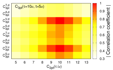
The correlation coefficients between the various $C_{\textrm{3pt}}$ measured at $t=\tau/2=5a$ and the $C_{\textrm{2pt}}$ at various values of $\tau$, are shown in Fig. 1. The strongest correlation is with the value of $C_{\textrm{2pt}}$ near the sink of $C_{\textrm{3pt}}$ at $\tau=10a$, and not near the $t=5a$ of operator insertion. Our intuitive understanding of why the correlation is strongest with $C_{\textrm{2pt}}(10a)$ is as follows: the spectral decompositions of the two correlation functions are similar except for the insertion of the operator at $t=5a$ in $C_{\textrm{3pt}}(10a)$. If the ground state saturates these correlation functions, then the extra term in $C_{\textrm{3pt}}$ is the matrix element of this operator within the ground state of the proton. This matrix element can be considered as inserting a number (the charge) at $t=5a$ in $C_{\textrm{2pt}}$. If the configuration to configuration fluctuations in the matrix element are small, then one expects a strong correlation between $C_{\textrm{2pt}}(10a)$ and $C_{\textrm{3pt}}(10a)$. In addition, there are strong correlations between successive time slices of $C_{\textrm{2pt}}$; thus, one expects the correlation of $C_{\textrm{3pt}}(10a)$ with $C_{\textrm{2pt}}$ to be spread over a few time slices about $t=10a$ as also indicated by the data in Fig. 1. In the more realistic case, in which the nucleon wave function at $t=5a$ has significant contributions from a tower of excited states, the operator can also cause transitions between these states, and its insertion can no longer be approximated by just one number. One can still expect that operators for which these transition matrix elements are small will have stronger correlations. Based on the observed pattern of excited states, discussed in Ref. Gupta et al. (2018), we expect the ordering of correlations $V>T>A>S$, whereas the observed pattern shown in Fig. 1 is $V>S>T>A$.

It is the existence of such correlations that allows the prediction of $C_{\textrm{3pt}}$ from $C_{\textrm{2pt}}$ using a boosted decision tree (BDT) regression algorithm available in SCIKIT-LEARN PYTHON ML library Pedregosa et al. (2011). BDT is a ML algorithm that builds an ensemble (tower) of simple decision trees such that each successive decision tree corrects the prediction error of the previous decision tree. The result is a powerful regression algorithm with small number of tuning parameters and a low risk of overfitting. It is also fast: for the data sizes we are considering, it only takes a couple of minutes on a laptop to find an appropriate predictor and evaluate it on the unlabeled samples. The SCIKIT-LEARN implementation of the BDT we used in this study is based on the Classification and Regression Trees (CART) algorithm Breiman et al. (1984) with gradient boosting Friedman (2000, 2002). For the prediction of $C_{\textrm{3pt}}$, we use 100 boosting stages of depth-3 trees with learning rate of 0.1 and a subsampling of 0.7. Note that, in this example, the pattern of correlation is such that a linear regression algorithm (such as LASSO Santosa and Symes (1986); Tibshirani (1994) or RIDGE Hoerl and Kennard (1970)) gives predictions with reasonable precision. Such a simplification does not occur for the second example described later.

$\Gamma$	DM	${\cal P}1$	Bias	Prediction
				without BC
S	0.936(10)	0.933(15)	$+$0.002(46)	0.934(14)
A	1.2011(41)	1.1997(48)	$-$0.0003(105)	1.1999(46)
T	1.0627(34)	1.0638(39)	$-$0.0004(78)	1.0636(38)
V	1.0462(36)	1.0455(36)	$+$0.0002(20)	1.0456(36)

Table 1: Average of $C_{\textrm{3pt}}^{\Gamma}(10a,5a)/\langle C_{\textrm{2pt}}(10a)\rangle$ on the unlabeled dataset. DM is the directly measured result, ${\cal P}1$ is the BC prediction defined in the text, with the bias correction factor given in column 4. For the prediction without BC, we used the full 680 labeled configurations for training of the BDT. Note that for this large dataset, the bias correction and the increase in the error in the prediction with BC are negligible.

The outline of the calculation is as follows:

1. For each $(\tau,t)$, the BDT is trained using the set of $C_{\textrm{2pt}}$ data (input) and $C_{\textrm{3pt}}^{A,S,T,V}(\tau,t)$ (output). This trained BDT can now take as input the unseen $C_{\textrm{2pt}}$ data and output the predicted $C_{\textrm{3pt}}^{A,S,T,V}(\tau,t)$. To predict $C_{\textrm{3pt}}$ at a given $(\tau,t)$, one can use the data for $C_{\textrm{2pt}}$ on all time slices. The essence of a trained BDT is that it gives larger weight to the input $C_{\textrm{2pt}}$ element with higher correlation with the target observable.

2. The trained BDT is first used on the dataset designated for BC data to predict $C_{\textrm{3pt}}^{A,S,T,V}(\tau,t)$. The bias correction factor is then determined by comparing this prediction with the corresponding directly measured value on the same BC set.

3. The trained BDT is next used on the unlabeled $C_{\textrm{2pt}}$ dataset to give the predicted $C_{\textrm{3pt}}^{A,S,T,V}(\tau,t)$.

4. To the average of this predicted $C_{\textrm{3pt}}^{A,S,T,V}(\tau,t)$ set, the bias correction factor is added to give the BC prediction we call ${\cal{P}}1$.

5. The statistical precision can be improved by constructing the weighted average of the BC prediction ${\cal{P}}1$ and the direct measured (DM) results on the labeled dataset. We call this estimate ${\cal{P}}2$. Note that the direct measurements on the labeled data and the predictions on the unlabeled data are not identically distributed because the prediction is not exact, however, the bias-corrected mean is the same. Therefore, when performing excited-state fits discussed below, we simultaneously fit the two data sets with common fit parameters.

The training and prediction steps treat data from each source position as independent, whereas the bias-corrected estimates for each bootstrap sample are obtained using configuration averages in Eq. (1). In this case, the errors are obtained using 500 bootstrap samples.

For the first example, we choose 680 of the 2263 configurations, separated by three configurations in trajectory order, as the labeled data. To determine the number of configurations to use for training, we varied the number between 30 and 180. We found that the variance of the prediction on the unlabeled dataset was the smallest and roughly constant between 60 and 120. We, therefore, picked 60 configurations from the labeled set for training and 620 for bias correction. The 1583 unlabeled configurations were used for prediction. The BDT regression algorithm was trained to predict $C_{\textrm{3pt}}^{A,S,T,V}(\tau,t)/{\cal N}$ for all $\tau$ and $t$ with $\{C_{\textrm{2pt}}(\tau)/{\cal N}\textrm{ for }\tau/a=0,1,2,\ldots,20\}$ as input. The normalization ${\cal N}\equiv{\langle{C_{\textrm{2pt}}(\tau)}\rangle}$ was needed to make numbers of $O(1)$ for numerical stability of the BDT in the SCIKIT-LEARN library.

Figure 2: Statistical distribution of $C_{\textrm{3pt}}(10a,5a)$ (light gold) and the prediction error (dark red). The ratios of the standard deviations of the prediction error (PE) and DM data at $t=\tau/2=5a$ are ${\sigma_{\textrm{PE}}/\sigma_{\textrm{DM}}}$ = 0.79, 0.49, 0.44 and 0.12 for S, A, T and V, respectively.

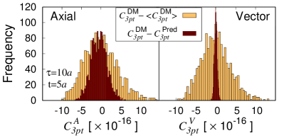
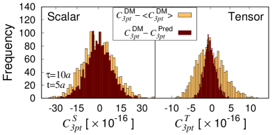
Data in Table 1 show that the statistical errors in the bias correction term are large; however, the error in the BC estimate is essentially identical to that in the DM estimates. This implies strong correlations between the two terms, uncorrected and the BC factor. Fig. 2 shows that the statistical fluctuations in the DM data are larger than the prediction error (PE $\equiv C_{\textrm{3pt}}^{\rm DM}-C_{\textrm{3pt}}^{\rm Pred}$) of the ML algorithm. The ratios of the standard deviations, ${\sigma_{\textrm{PE}}/\sigma_{\textrm{DM}}}$, of the PE and DM data are given in Table 2. This pattern of smaller variance leads us to believe that, with further optimization, the reduction in computation cost given in Table 4 can be increased significantly.

${\sigma_{\textrm{PE}}/\sigma_{\textrm{DM}}}$ of ${\cal P}2$
$\Gamma$	$\tau=8$	$\tau=10$	$\tau=12$	$\tau=14$
S	0.791(16)	0.793(15)	0.791(14)	0.785(14)
A	0.394(9)	0.493(12)	0.601(13)	0.721(14)
T	0.334(9)	0.439(11)	0.571(13)	0.705(14)
V	0.089(4)	0.115(8)	0.134(7)	0.159(6)
${\sigma_{\textrm{PE}}/\sigma_{\textrm{DM}}}$ of ${\cal VP}2$
$\Gamma$	$\tau=8$	$\tau=10$	$\tau=12$	$\tau=14$
S	0.696(14)	0.535(12)	input	0.546(12)
A	0.357(9)	0.355(9)	input	0.501(12)
T	0.304(8)	0.329(9)	input	0.498(12)
V	0.089(5)	0.105(10)	input	0.143(7)

Table 2: Ratio ${\sigma_{\textrm{PE}}/\sigma_{\textrm{DM}}}$ representing quality of the prediction ${\cal P}2$ (upper) and ${\cal VP}2$ (lower) at $t=\tau/2$. Smaller values indicate better prediction.

We have carried out two kinds of tests of the efficacy of the method. In Table 3, we show data for $C_{\textrm{3pt}}^{\Gamma}(10a,5a)/\langle C_{\textrm{2pt}}(10a)\rangle$ for different numbers of labeled data, keeping (i) the full $2263$ configurations and (ii) 500 configurations. We find that the results are consistent for different numbers, Prediction($N,N_{t}$), of labeled data in both cases. Even when only ten configurations (640 measurements) are used for the training dataset, one gets reasonable estimates. The errors scale roughly as the total number of configurations as can be seen by comparing the upper and lower tables.

Total number of configurations: 2263
$\Gamma$	DM	Prediction	Prediction	Prediction
		(680,60)	(450,40)	(225,20)
S	0.930(09)	0.925(14)	0.937(19)	0.959(26)
A	1.1984(33)	1.1967(42)	1.1991(52)	1.2046(69)
T	1.0611(27)	1.0615(35)	1.0637(40)	1.0659(51)
V	1.0437(28)	1.0427(28)	1.0437(31)	1.0434(32)
Total number of configurations: 500
$\Gamma$	DM	Prediction	Prediction	Prediction
		(150,20)	(100,20)	(50,10)
S	0.935(19)	0.904(29)	0.909(32)	0.988(40)
A	1.1940(77)	1.1848(99)	1.188(11)	1.191(17)
T	1.0588(62)	1.0663(78)	1.0555(88)	1.0495(112)
V	1.0437(64)	1.0429(64)	1.0417(63)	1.0443(70)

Table 3: Average of $C_{\textrm{3pt}}^{\Gamma}(10a,5a)/\langle C_{\textrm{2pt}}(10a)\rangle$ on the full dataset of 2263 (upper) and 500 (lower) configurations. Prediction($N,N_{t}$) denotes predictions made using $N$ labeled configurations of which $N_{t}$ are used for training.

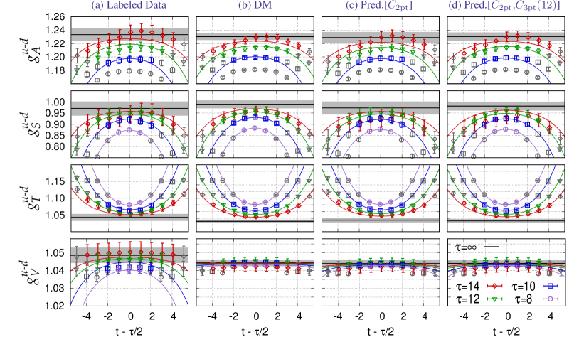
In Fig. 3, we compare the prediction ${\cal{P}}2$ of $C_{\textrm{3pt}}^{A,S,T,V}$ at all $\tau$ and $t$ [column (c)] with the DM on labeled and full data shown in columns (a) and (b), respectively. The observed dependence on $\tau$ and $t$ is due to contributions from excited states of the nucleon, and the desired ground-state result is given by the limit $\tau\to\infty$. This can be obtained by fitting the data at various $t$ and $\tau$ using the spectral decomposition of $C_{\textrm{3pt}}^{A,S,T,V}$. Fig. 3 shows such a fit assuming only the lowest two states contribute to the spectral decomposition, i.e., the two-state fit described in Refs. Bhattacharya et al. (2014); Gupta et al. (2018); Bhattacharya et al. (2016a). The lines show the result of this fit for the various $\tau$, and the gray band gives the $\tau\to\infty$ value. We find that the prediction ${\cal{P}}2$ in column (c) is consistent with the DM results on the full dataset.

We can further improve the prediction if data for a single value of $\tau$, say $C_{\textrm{3pt}}^{A,S,T,V}(\tau/a=12)$, is available on the full dataset. Then, in the training stage, we use as input both $C_{\textrm{2pt}}$ and $C_{\textrm{3pt}}^{A,S,T,V}(\tau/a=12)$. Having trained the BDT on the labeled data, we now use $C_{\textrm{2pt}}$ and $C_{\textrm{3pt}}^{A,S,T,V}(\tau/a=12)$ as input to predict $C_{\textrm{3pt}}(\tau/a=8,10,14)$, which we label ${\cal{VP}}2$. These results are shown in Fig. 3 column (d). Including $C_{\textrm{3pt}}^{A,S,T,V}(\tau/a=12)$ in the training and the prediction stages increases the computational cost relative to ${\cal{P}}2$ but reduces the errors. For a fixed size of error, ${\cal{VP}}2$ is more efficient than ${\cal{P}}2$ as shown in Table 4.

A comparison of the predictions from $C_{\textrm{2pt}}$ (${\cal P}2$) and from $C_{\textrm{2pt}}$ and $C_{\textrm{3pt}}^{A,S,T,V}(\tau/a=12)$ (${\cal VP}2$) vs DM is shown in Table 4 for the charges $g_{A,S,T,V}$ obtained after the extrapolation $\tau\to\infty$ using the four values of $\tau$. While both estimates, ${\cal P}2$ and ${\cal VP}2$, are consistent with the DM, ${\cal VP}2$ is closer to DM with respect to both the central value and the error. Taking into account the increase in the statistical uncertainty (scaling the cost by the square of the number of measurements) in the predicted results, the ML analysis ${\cal VP}2$ provides between a 7% and 26% reduction in the computational cost. The amount of gain is observable dependent.

Figure 3: Removing excited-state contamination using the two-state fit for (a) DM on the labeled data, (b) DM on full data, (c) DM on labeled data combined with ML predictions from $C_{\textrm{2pt}}$ on unlabeled data (${\cal{P}}2$), and (d) DM on labeled data combined with ML predictions from $C_{\textrm{2pt}}$ and $C_{\textrm{3pt}}(\tau=12a)$ on unlabeled data (${\cal{VP}}2$).

	DM	${\cal{P}}2(\tau\to\infty)$	Cost(%)	${\cal{VP}}2(\tau\to\infty)$	Cost(%)
		[$C_{\textrm{2pt}}$]		[$C_{\textrm{2pt}}$,$C_{\textrm{3pt}}$(12)]
$g_{S}$	0.989(18)	0.973(29)	138	0.981(20)	80
$g_{A}$	1.2303(51)	1.2289(83)	141	1.2304(61)	93
$g_{T}$	1.0311(51)	1.0347(68)	97	1.0326(54)	74
$g_{V}$	1.0443(19)	1.0439(22)	74	1.0440(21)	78

Table 4: Comparison of $\tau\to\infty$ extrapolated nucleon charges calculated from the ML predictions ${\cal{P}}2$ and ${\cal{VP}}2$ and the relative computational cost vs the DM. The cost includes the factor required to make the errors the same assuming they scale as $M^{2}$.

III Experiment B: CP violating phase in the Neutron State

The second example is taken from the calculation of the matrix element of the chromoelectric dipole moment (cEDM) operator, ${O_{\textrm{cEDM}}{\equiv}i\bar{q}(\sigma_{\mu\nu}G^{\mu\nu})\gamma_{5}q}$ where $G^{\mu\nu}$ is the gluon field strength tensor, within the neutron state. It arises in theories beyond the standard model and violates parity P and time-reversal T symmetries, or equivalently, charge C and CP symmetries in theories invariant under CPT. Since any CP violating (CPV) operator gives a contribution to the neutron electric dipole moment (nEDM), a bound or a nonzero value for nEDM in coming experiments will constrain novel CP violation Pospelov and Ritz (2005); Ramsey-Musolf and Su (2008); Engel et al. (2013). So far only preliminary lattice QCD calculations exist and cost-effectively improving the statistical signal is essential Syritsyn et al. (2018); Kim et al. (2018); Bhattacharya et al. (2018). We have proposed a Schwinger source method approach (SSM) Bhattacharya et al. (2016b, c) that exploits the fact that the cEDM operator is a quark bilinear. In the SSM, effects of the cEDM interaction are incorporated into the two- and three-point functions by modifying the Dirac clover fermion action:

$$D_{\text{clov}} \rightarrow D_{\text{clov}}+i\varepsilon\sigma_{\mu\nu}\gamma_{5}G^{\mu\nu}$$

$$D_{\text{clov}} \rightarrow D_{\text{clov}}+i\varepsilon_{5}\gamma_{5}\,.$$ (3)

The second equation is for the pseudoscalar operator $O_{\gamma_{5}}{\equiv}i\bar{q}\gamma_{5}q$ that mixes with cEDM due to quantum effects Bhattacharya et al. (2015b).

With CP violation, the Dirac equation for the neutron spinor $u$ becomes $(ip_{\mu}\gamma_{\mu}+me^{-i2\alpha\gamma_{5}})u=0$; i.e., the neutron spinor acquires a CP-odd phase $\alpha$ ($\alpha_{5}$), which is expected to be linear in $\varepsilon$ ($\varepsilon_{5}$) for small $\varepsilon$ ($\varepsilon_{5}$). At leading order, these phases can be obtained from the four two-point functions, $C_{\text{2pt}}$, $C_{\text{2pt}}^{P}$, $C_{\text{2pt}}^{P,\varepsilon}$, and $C_{\text{2pt}}^{P,\varepsilon_{5}}$, where the superscript $P$ indicates an additional factor of $\gamma_{5}$ is included in the spin projection Shintani et al. (2016); Bhattacharya et al. (2018). The correlator $C_{\text{2pt}}^{P,\varepsilon}$ ( $C_{\text{2pt}}^{P,\varepsilon_{5}}$) is constructed using quark propagators with the $O_{\textrm{cEDM}}$ ($O_{\gamma_{5}}$) term and is expected to be imaginary and vanish as $\varepsilon\to 0$ ($\varepsilon_{5}\to 0$). In a first step, we show predictions of the BDT regression algorithm for these two using only $C_{\text{2pt}}$ and $C_{\text{2pt}}^{P}$.

For the training and prediction, we use the $C_{\text{2pt}}$, $C_{\text{2pt}}^{P}$, $C_{\text{2pt}}^{P,\varepsilon}$ and $C_{\text{2pt}}^{P,\varepsilon_{5}}$ measured in Refs. Bhattacharya et al. (2016b, c) on 400 MILC highly improved staggered quarks (HISQ) lattices at $a=0.12$ fm and $M_{\pi}=310$ MeV (the $a12m310$ ensemble) with clover fermions. On each configuration, these correlators are constructed using 64 randomly chosen widely separated sources with a sloppy stopping condition, the effects of which are again ignored. Out of the 400 configurations, 120 configurations, separated by three configurations in trajectory order, are chosen as the labeled data, and the remaining 280 configurations are used as the unlabeled data. From the labeled data, 70 randomly chosen configurations are used for training. Only 50 configurations sufficed for bias correction in this case because the ratio of standard deviations of the prediction error vs the DM (${\sigma_{\textrm{PE}}/\sigma_{\textrm{DM}}}$) is small as shown in Fig. 4. Errors are obtained using 200 bootstrap samples.

Figure 4: Distribution of $\operatorname{Im}\big{[}C_{\textrm{2pt}}^{P,\varepsilon}(10a)\big{]}$ (left) and $\operatorname{Im}\big{[}C_{\textrm{2pt}}^{P,\varepsilon_{5}}(10a)\big{]}$ (right), averaged over sources in each configuration, are shown in light gold and the prediction error in dark red. The ratio of the standard deviations $\sigma_{\textrm{PE}}/\sigma_{\textrm{2pt}}\approx$ 0.18 for $O_{\textrm{cEDM}}$ and 0.4 for $O_{\gamma_{5}}$.

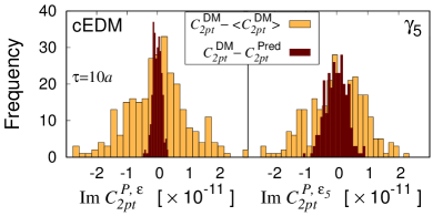
The BDT regression algorithm is trained to predict the imaginary parts of $C_{\text{2pt}}^{P,\varepsilon}$ and $C_{\text{2pt}}^{P,\varepsilon_{5}}$ using both the real and imaginary parts of $C_{\text{2pt}}$ and $C_{\text{2pt}}^{P}$. Note that in the absence of the CPV terms, $C_{\text{2pt}}^{P}$ and the imaginary part of $C_{\text{2pt}}$ average to zero, but, they have nonzero correlations with the target imaginary parts of $C_{\text{2pt}}^{P,\varepsilon}$ and $C_{\text{2pt}}^{P,\varepsilon_{5}}$. The BDT regression algorithm with 500 boosting stages of depth-3 trees with learning rate of 0.1 and subsampling of 0.7 gives a good prediction as shown in Fig. 4. Because of nonlinear correlations, the BDT works better than linear regression algorithms in this case; the prediction error is about 50% larger with linear models at $t=1$ and decreases to less than 10% by $t=8$. Again, for numerical stability, all data fed into the BDT algorithm are normalized by $\langle{C_{\text{2pt}}(\tau)}\rangle$.

Figure 5: CPV phase $\alpha$ calculated from the DM $C_{\text{2pt}}^{P}$ on the full data (red squares), improved ML prediction (blue circles), and the labeled data (green triangles).

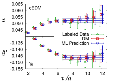
Using the predicted $C_{\text{2pt}}^{P,\varepsilon}$ and $C_{\text{2pt}}^{P,\varepsilon_{5}}$ on all time slices, we calculate the CPV phases $\alpha$ and $\alpha_{5}$ by taking their ratio with $C_{\text{2pt}}$, because $C_{\text{2pt}}^{\varepsilon,\varepsilon_{5}}$ differ from $C_{\text{2pt}}$ at $O(\varepsilon^{2})$. Fig. 5 shows the comparison between the CPV phase calculated from DM on the full and labeled data and the ML predicted data. The horizontal lines give the averages over the plateau region where the excited-state contamination is small. Results for $\alpha$ and $\alpha_{5}$ are summarized in Table 5. To get the improved ML predictions, we combine the prediction on the 280 unlabeled configurations with the DM data on the 120 labeled configurations. These combined data are analyzed following the same bootstrap resampling procedure used in the first example discussed earlier.

The prediction uses 30% of the data for $C_{\text{2pt}}^{P,\varepsilon}$ and $C_{\text{2pt}}^{P,\varepsilon_{5}}$ and 100% for $C_{\text{2pt}}^{P}$ and $C_{\text{2pt}}$. This reduces the total number of propagator calculations by 47% compared to the direct measurement. Taking into account the increase of the statistical uncertainty, the computational cost reduction is about 30% as shown in Table 5.

	DM	${\cal{P}}2$	Cost
$\alpha$	$+$0.0527(17)	$+$0.0525(18)	62%
$\alpha_{5}$	$-$0.1463(14)	$-$0.1460(17)	77%

Table 5: Comparison of the ML prediction of the CPV phases $\alpha$ and $\alpha_{5}$ and the relative cost vs the DM results.

IV Conclusion

In conclusion, the proposed ML algorithm used to predict compute-intensive observables from simpler measurements gives a modest computational cost reduction of 7%–38% depending on the observables analyzed here as summarized in Tables 4 (${\cal{VP}}2$) and 5 (${\cal{P}}2$). The technique is, however, general provided one can find inexpensive measurements that correlate well with the observable of interest. The computational cost reduction depends on the degree of correlations. We are investigating other ML methods to further improve the quality of the prediction and reduce computational cost.

Appendix A Example python code for machine learning regression

A simplified example of the python code used for ML training and prediction, using a BDT regression algorithm provided by the SCIKIT-LEARN library Pedregosa et al. (2011), is given in Listing 1. The code shows the calls for importing the SCIKIT-LEARN module, defining and training the BDT regressor, making predictions using the trained regressor, and implementing the BC procedure. Here we assumed that the required training, BC, and unlabeled data are given by a LOAD_DATA() function. The bootstrap procedure, needed to estimate uncertainty of the final BC prediction, is implicitly wrapped around the various calls in the code in Listing 1 as described in Section I.

⬇

1import numpy as np

2from sklearn.ensemble import GradientBoostingRegressor

3

4# Load data

5# X_i = [o1_i, o2_i, o3_i, …]; Array of measured observables

6# y_i = O_i ; DM of target observable O

7# X_train, X_bc, X_unlab: arrays of X_i

8# y_train, y_bc : arrays of y_i

9X_train, y_train, X_bc, y_bc, X_unlab = LOAD_DATA()

10

11# Gradient boosted decision tree regressor

12gbr = GradientBoostingRegressor(learning_rate=0.1, n_estimators=100, max_depth=3)

13

14# Training regressor to predict y_i from X_i

15gbr.fit(X_train, y_train)

16

17# Predictions of y on bias correction and unlabeled datasets

18y_bc_pred = gbr.predict(X_bc)

19y_unlab_pred = gbr.predict(X_unlab)

20

21# Bias correction term

22BiasCrxn = np.average(y_bc - y_bc_pred)

23

24# Predictions on unlabeled dataset given by the average

25PredAvg = np.average(y_unlab_pred)

26

27# Bias-corrected prediction of <O>

28BC_Pred = PredAvg + BiasCrxn

Listing 1: Python example code for calculating bias-corrected predictions using BDT in scikit-learn library. In the code, we assume that the data is given by LOAD_DATA() function.

References

- Wilson (1974) K. G. Wilson, Phys. Rev. D10, 2445 (1974), [,319(1974)].
- Creutz (1980) M. Creutz, Phys. Rev. D21, 2308 (1980).
- Bali et al. (2010) G. S. Bali, S. Collins, and A. Schafer, Comput. Phys. Commun. 181, 1570 (2010), eprint 0910.3970.
- Blum et al. (2013) T. Blum, T. Izubuchi, and E. Shintani, Phys. Rev. D88, 094503 (2013), eprint 1208.4349.
- Baldi et al. (2014) P. Baldi, P. Sadowski, and D. Whiteson, Nature Commun. 5, 4308 (2014), eprint 1402.4735.
- Baldi et al. (2015) P. Baldi, P. Sadowski, and D. Whiteson, Phys. Rev. Lett. 114, 111801 (2015), eprint 1410.3469.
- Alexandru et al. (2017) A. Alexandru, P. F. Bedaque, H. Lamm, and S. Lawrence, Phys. Rev. D96, 094505 (2017), eprint 1709.01971.
- Wetzel and Scherzer (2017) S. J. Wetzel and M. Scherzer, Phys. Rev. B96, 184410 (2017), eprint 1705.05582.
- Shanahan et al. (2018) P. E. Shanahan, D. Trewartha, and W. Detmold (2018), eprint 1801.05784.
- Efron (1979) B. Efron, The Annals of Statistics 7, 1 (1979), ISSN 00905364, URL http://www.jstor.org/stable/2958830.
- Gupta et al. (2018) R. Gupta, Y.-C. Jang, B. Yoon, H.-W. Lin, V. Cirigliano, and T. Bhattacharya (2018), eprint 1806.09006.
- Bhattacharya et al. (2016a) T. Bhattacharya, V. Cirigliano, S. Cohen, R. Gupta, H.-W. Lin, and B. Yoon, Phys. Rev. D94, 054508 (2016a), eprint 1606.07049.
- Bhattacharya et al. (2012) T. Bhattacharya, V. Cirigliano, S. D. Cohen, A. Filipuzzi, M. Gonzalez-Alonso, M. L. Graesser, R. Gupta, and H.-W. Lin, Phys. Rev. D85, 054512 (2012), eprint 1110.6448.
- Bhattacharya et al. (2015a) T. Bhattacharya, V. Cirigliano, R. Gupta, H.-W. Lin, and B. Yoon, Phys. Rev. Lett. 115, 212002 (2015a), eprint 1506.04196.
- Follana et al. (2007) E. Follana, Q. Mason, C. Davies, K. Hornbostel, G. P. Lepage, J. Shigemitsu, H. Trottier, and K. Wong (HPQCD, UKQCD), Phys. Rev. D75, 054502 (2007), eprint hep-lat/0610092.
- Bazavov et al. (2013) A. Bazavov et al. (MILC), Phys. Rev. D87, 054505 (2013), eprint 1212.4768.
- Babich et al. (2010) R. Babich, J. Brannick, R. C. Brower, M. A. Clark, T. A. Manteuffel, S. F. McCormick, J. C. Osborn, and C. Rebbi, Phys. Rev. Lett. 105, 201602 (2010), eprint 1005.3043.
- Osborn et al. (2010) J. C. Osborn, R. Babich, J. Brannick, R. C. Brower, M. A. Clark, S. D. Cohen, and C. Rebbi, PoS LATTICE2010, 037 (2010), eprint 1011.2775.
- Edwards and Joo (2005) R. G. Edwards and B. Joo (SciDAC, LHPC, UKQCD), Nucl. Phys. Proc. Suppl. 140, 832 (2005), [,832(2004)], eprint hep-lat/0409003.
- Yoon et al. (2016) B. Yoon et al., Phys. Rev. D93, 114506 (2016), eprint 1602.07737.
- Pedregosa et al. (2011) F. Pedregosa, G. Varoquaux, A. Gramfort, V. Michel, B. Thirion, O. Grisel, M. Blondel, P. Prettenhofer, R. Weiss, V. Dubourg, et al., Journal of Machine Learning Research 12, 2825 (2011).
- Breiman et al. (1984) L. Breiman, J. Friedman, C. Stone, and R. Olshen, Classification and Regression Trees, The Wadsworth and Brooks-Cole statistics-probability series (Taylor & Francis, 1984), ISBN 9780412048418, URL https://books.google.com/books?id=JwQx-WOmSyQC.
- Friedman (2000) J. H. Friedman, Annals of Statistics 29, 1189 (2000).
- Friedman (2002) J. H. Friedman, Comput. Stat. Data Anal. 38, 367 (2002), ISSN 0167-9473, URL http://dx.doi.org/10.1016/S0167-9473(01)00065-2.
- Santosa and Symes (1986) F. Santosa and W. W. Symes, SIAM J. Sci. and Stat. Comput. 7(4), 1307 (1986).
- Tibshirani (1994) R. Tibshirani, Journal of the Royal Statistical Society. Series B 58, 267 (1994).
- Hoerl and Kennard (1970) A. E. Hoerl and R. W. Kennard, Technometrics 12, 55 (1970).
- Bhattacharya et al. (2014) T. Bhattacharya, S. D. Cohen, R. Gupta, A. Joseph, H.-W. Lin, and B. Yoon, Phys. Rev. D89, 094502 (2014), eprint 1306.5435.
- Pospelov and Ritz (2005) M. Pospelov and A. Ritz, Annals Phys. 318, 119 (2005), eprint hep-ph/0504231.
- Ramsey-Musolf and Su (2008) M. J. Ramsey-Musolf and S. Su, Phys. Rept. 456, 1 (2008), eprint hep-ph/0612057.
- Engel et al. (2013) J. Engel, M. J. Ramsey-Musolf, and U. van Kolck, Prog. Part. Nucl. Phys. 71, 21 (2013), eprint 1303.2371.
- Syritsyn et al. (2018) S. Syritsyn, T. Izubuchi, and H. Ohki, in 13th Conference on the Intersections of Particle and Nuclear Physics (CIPANP 2018) Palm Springs, California, USA, May 29-June 3, 2018 (2018), eprint 1810.03721.
- Kim et al. (2018) J. Kim, J. Dragos, A. Shindler, T. Luu, and J. de Vries, in 36th International Symposium on Lattice Field Theory (Lattice 2018) East Lansing, MI, United States, July 22-28, 2018 (2018), eprint 1810.10301.
- Bhattacharya et al. (2018) T. Bhattacharya, B. Yoon, R. Gupta, and V. Cirigliano, in 36th International Symposium on Lattice Field Theory (Lattice 2018) East Lansing, MI, United States, July 22-28, 2018 (2018), eprint 1812.06233.
- Bhattacharya et al. (2016b) T. Bhattacharya, V. Cirigliano, R. Gupta, E. Mereghetti, and B. Yoon, PoS LATTICE2015, 238 (2016b), eprint 1601.02264.
- Bhattacharya et al. (2016c) T. Bhattacharya, V. Cirigliano, R. Gupta, and B. Yoon, PoS LATTICE2016, 225 (2016c), eprint 1612.08438.
- Bhattacharya et al. (2015b) T. Bhattacharya, V. Cirigliano, R. Gupta, E. Mereghetti, and B. Yoon, Phys. Rev. D92, 114026 (2015b), eprint 1502.07325.
- Shintani et al. (2016) E. Shintani, T. Blum, T. Izubuchi, and A. Soni, Phys. Rev. D93, 094503 (2016), eprint 1512.00566.