Evolving Differentiable Gene Regulatory Networks

Abstract

Over the past twenty years, artificial Gene Regulatory Networks (GRNs) have shown their capacity to solve real-world problems in various domains such as agent control, signal processing and artificial life experiments. They have also benefited from new evolutionary approaches and improvements to dynamic which have increased their optimization efficiency. In this paper, we present an additional step toward their usability in machine learning applications. We detail an GPU-based implementation of differentiable GRNs, allowing for local optimization of GRN architectures with stochastic gradient descent (SGD). Using a standard machine learning dataset, we evaluate the ways in which evolution and SGD can be combined to further GRN optimization. We compare these approaches with neural network models trained by SGD and with support vector machines.

1 Introduction

Artificial Gene Regulatory Networks (GRNs) have varied in implementation since their conception, with initial boolean network representations that directly encode connections giving way to proteins that interpolate their connection using exponential or other functions. Following inspiration from biology, these models have been optimized using genetic algorithms, with advances in GRN representation often involving improvements to the evolvability of the representation [Kuo et al., 2004], [Cussat-Blanc et al., 2015], [Disset et al., 2017].

Artificial GRNs were first proposed using a binary encoding of proteins with specific start and stop codons, similar to biological genetic encoding [Banzhaf, 2003]. GRNs have since been used in a number of domains, including robot control [Joachimczak and Wrobel, 2010], signal processing [Joachimczak and Wróbel, 2010], wind farm design, [Wilson et al., 2013], and reinforcement learning [Cussat-Blanc and Harrington, 2015]. Finding similar use to their biological inspiration, GRNs have controlled the design and development of multi-cellular creatures [Cussat-Blanc et al., 2008] and of artificial neural networks (ANNs) [Wróbel and Abdelmotaleb, 2012]. Evolution and dynamics were recently improved in [Cussat-Blanc et al., 2015, Disset et al., 2017]. Artificial GRNs have also been used to investigate a number of questions in the context of evolution. A strong relationship was shown between their robustness against noise and against genetic material deletions [Rohlf and Winkler, 2009]. Redundancy of genetic material was proven to enhance evolvability up to a point [Schramm et al., 2012] and it was shown that modular genotypes can emerge when GRNs are subjected to dynamic fitness landscapes [Lipson et al., 2002].

In this paper, we present a model that takes the process of optimizing GRNs one step further, by introducing the differentiable Gene Regulatory Network, a GRN capable of learning. We show that differentiable GRNs benefit from a combination of evolution and learning. The availability of modern platforms capable of performing gradient descent with complex functions has enabled this work. A differentiable GRN written using TensorFlow is presented. For ease of comparison with and incorporation into existing learning models, especially deep neural networks, the GRN has been implemented as a Keras layer. This implementation is available in an open-source repository.

This paper also aims at studying the relationship between evolution and learning using GRNs. While this constitutes a first look with GRNs (to the best of our knownledge), ANNs have been used to understand both the Baldwin effect and Lamarckian evolution. ANNs have been evolved with the option of allowing certain weights to be learned, demonstrating that learning can improve evolution’s ability to reach difficult parts of the search space [Hinton and Nowlan, 1987]. Lamarckian evolution has been used to combine evolution of the structure of a Complex Pattern Producing Network and learning of the network’s weights [Fernando et al., 2016]. This work intends to explore the relationship between evolution and learning in the context of GRNs, which are detailed next.

Plasticity is an adaptive response variation that allows an organism to respond to environmental change. The evolutionary advantage of plasticity was first proposed in [Baldwin, 1896] and is now referred to as the Baldwin Effect. The Baldwin Effect suggests that learned/adaptive behaviors which have fitness advantages can facilitate the genetic assimilation of equivalent behaviors by subsequent generations. The Baldwin Effect has been studied in a number of systems, including RNA [Ancel et al., 2000], neural networks [Schemmel et al., 2006], and theoretical models [Ancel, 2000]. We suggest that GRNs which can change or “learn” over their lifetime may be influenced by the Baldwin effect; evolutionary selection based upon learning may produce a population in parts of the evolutionary search space which are difficult to reach without learning.

To this end, we first present the differentiable GRN model, transforming standard GRN equations into a series of differentiable matrix operations, and use this model to address some questions concerning the relationship between evolution and learning. The GRN model is uniquely poised to study aspects of this complex relationship, as evolutionary methods for the model have been well studied and as the entire genome is differentiable.

2 Implementation

A GRN is composed of multiple artificial proteins, which interact via evolved properties. These properties, called tags, are: the protein identifier, encoded as a floating point value between 0 and 1; the enhancer identifier, encoded as a floating point value between 0 and 1, which is used to calculate the enhancing matching factor between two proteins; the inhibitor identifier, encoded as a floating point value between 0 and 1, which is used to calculate the inhibiting matching factor between two proteins and; the type, either input, output, or regulator, which is a constant set by the user and is not evolved.

Each protein has a concentration, representing the use of this protein and providing state to the network. For input proteins, the concentration is given by the environment and is unaffected by other proteins. output protein concentrations are used to determine actions in the environment; these proteins do not affect others in the network. The bulk of the computation is performed by regulatory proteins, an internal protein whose concentration is influenced by other input and regulatory proteins.

We will first present the classic computation of the GRN dynamics, using equations found to be optimal in [Disset et al., 2017] on a number of problems. Following this overview, we will present the conversion of these equations into a set of differentiable matrix operations.

The dynamics of the GRN are calculated as follows. First, the absolute affinity of a protein $a$ with another protein $b$ is given by the enhancing factor $u^{+}_{ab}$ and the inhibiting $u^{-}_{ab}$:

$$u^{+}_{ij}=u_{size}-|enh_{j}-id_{i}|~{}~{};~{}~{}u^{-}_{ij}=u_{size}-|inh_{j}-id_{i}|$$ (1)

where $id_{x}$ is the identifier, $enh_{x}$ is the enhancer identifier and $inh_{x}$ is the inhibitor identifier of protein $x$. The maximum enhancing and inhibiting affinities between all protein pairs are determined and are used to calculate the relative affinity, which is here simply called the affinity:

$$A^{+}_{ij}=-\beta u^{+}_{ij}~{}~{};~{}~{}A^{-}_{ij}=-\beta u^{-}_{ij}$$ (2)

$\beta$ is one of two control parameters used in a GRN, both of which are described below.

These affinities are used to then calculate the enhancing and inhibiting influence of each protein, following

$$g_{i}=\frac{1}{N}\sum_{j}^{N}{c_{j}e^{A^{+}_{ij}}}~{}~{};~{}~{}h_{i}=\frac{1}{N}\sum_{j}^{N}{c_{j}e^{A^{-}_{ij}}}$$ (3)

where $g_{i}$ (resp. $h_{i}$) is the enhancing (resp. inhibiting) value for a protein $i$, $N$ is the number of proteins in the network, $c_{j}$ is the concentration of protein $j$.

The final modification of protein $i$ concentration is given by the following differential equation:

$$\frac{dc_{i}}{dt}=\frac{\delta(g_{i}-h_{i})}{\Phi}$$ (4)

where $\Phi$ is a function that normalizes the output and regulatory protein concentrations to sum to 1.

$\beta$ and $\delta$ are two constants that determine the speed of reaction of the regulatory network. The higher these values, the more sudden the transitions in the GRN. The lower they are, the smoother the transitions. In this work, the $\beta$ and $\delta$ parameters are both evolved as a part of the GRN chromosome and learned in the optimization of the differentiable GRN.

2.1 Differentiable GRN

In this representation of the GRN, protein tags are separated into three vectors based on their function, $\mathbf{id}$, identifier, $\mathbf{enh}$, enhancer, and $\mathbf{inh}$, inhibitor. This is their form in evolution and the evolved vectors serve as initial values for learning. Protein concentrations are also represented as a vector, following the same indexing as the protein tags. Initial value for protein concentrations is 0.

The protein tags are then tiled to create three matrices. The enhancing and inhibiting matrices are transposed, and the affinities are then calculated for each element of the matrix using broadcasting, to be expressed in the form of the net influence of a protein on another protein, referred to as the protein signatures, $S$:

$$A^{+}=-\beta|ENH-ID|~{}~{};~{}~{}A^{-}=-\beta|INH-ID|~{}~{};~{}~{}$$ (5)

$$S=e^{A^{+}}-e^{A^{-}}$$ (6)

The protein tags $\mathbf{id},\mathbf{enh},\mathbf{inh}$ are all optimized by learning, as well as the $\beta$ and $\delta$ GRN parameters. The protein tags are constrained during optimization to be in $[0.0,1.0]$, and $\beta$ and $\delta$ are constrained between the parameter values $[\beta_{min},\beta_{max}]$ and $[\delta_{min},\delta_{max}]$, which, for this run, were both $[0.05,2.0]$. Learning therefore directly augments evolutionary search in this work; evolution also optimizes the protein tags, $\beta$, and $\delta$, and is bound by the same constraints.

2.2 GRN layer

The differentiable GRN model is encoded as a Keras layer to facilitate use. Keras is a popular deep learning framework which includes many implemented layers, such as dense, convolutional, and recurrent neural network layers. Layers are added to a model class, which provides the interface for learning and evaluation. Here we consider the GRN layer calculation as compared to common neural network layers, shown in Figure 1. This is not how the layer is implemented, but is shown rather to demonstrate the difference between the GRN and existing layer types.

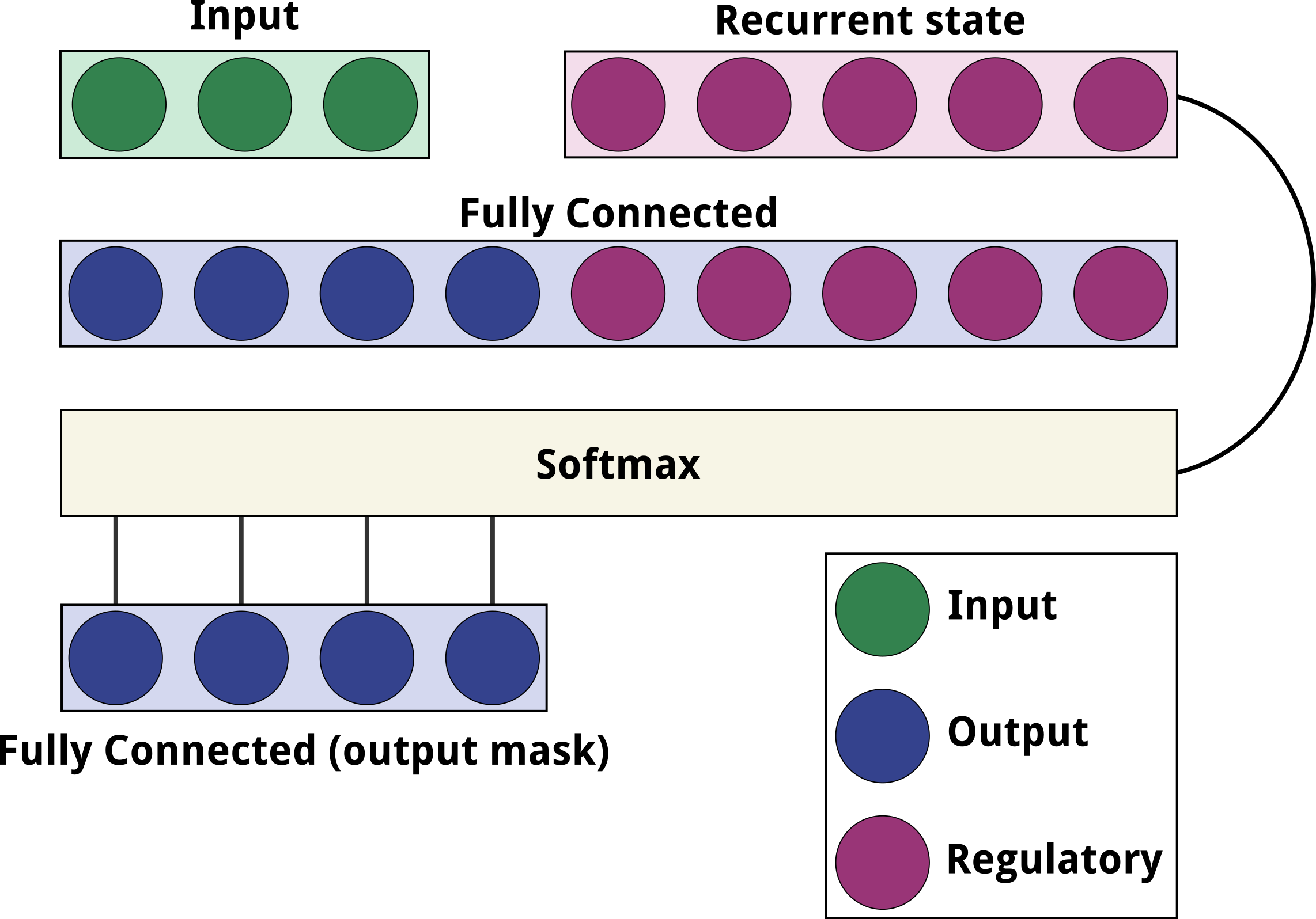
Figure 1: The GRN layer modeled as a composition of other layers

Input proteins influence output and regulatory proteins according to their respective signatures, which can be considered as weights; the first part of a GRN layer is therefore like a fully connected layer containing the output regulatory proteins. These protein concentrations are also influenced by the previous concentrations of the regulatory proteins, where the signatures from the regulatory proteins act as weights to all non-input proteins. Output proteins, however, do not influence regulatory proteins. The layer is therefore similar to a classic recurrent layer, in that nodes have non-zero weights between each other depending on their previous activation, but the state of this layer is stored in the regulatory proteins alone, not in the output proteins.

Finally, a large difference between a recurrent layer and the GRN is the normalization function, which can be modeled as a softmax layer. It is important to note that the softmax layer is applied before saving the state of the layer; the regulatory protein concentration which affects the next time-step is already normalized. Normalization has been shown to be an important part of artificial GRN evolution and use [Disset et al., 2017], however it may confound deep neural models not accustomed to having a softmax in the interior of the model. In Figure 2, a GRN layer with no normalization is considered.

Without normalization, the GRN layer resembles a classic recurrent layer containing the regulatory proteins followed by a fully connected layer containing the output proteins. However, as input proteins directly influence output proteins, there must be connections from the inputs to the fully connected output layer as well.

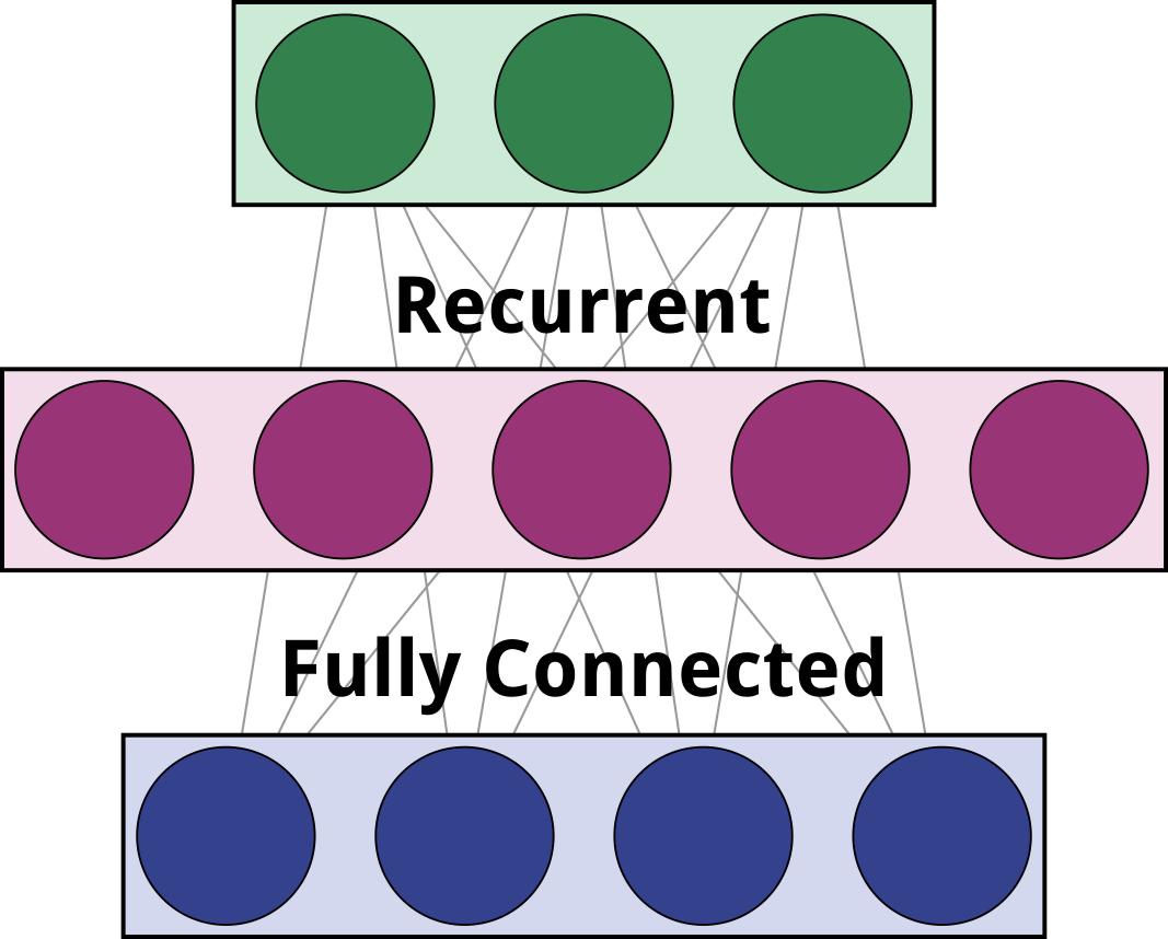
Figure 2: The GRN layer modeled as a composition of other layers, without protein concentration normalization

With these architectural comparisons in mind, the GRN layer resembles common neural network functions. Proteins behave as rectified linear units, as they are bound by 0 but otherwise apply no activation transformation. Unlike artificial neurons, however, GRN proteins have no bias; the activation is simply the sum of the weighted input. Finally, it is important to note that, while the signature matrix can be used to represent weights between nodes, the signature matrix was not optimized during training. Rather, the protein tags $\mathbf{id},\mathbf{enh},\mathbf{inh}$ are optimized by learning, as well as the $\beta$ and $\delta$ GRN parameters. The training is therefore constrained, similar to how convolutional layers use a kernel to represent multiple weights.

2.3 Evolution

The evolutionary method used in this work is the Gene Regulatory Network Evolution Through Augmenting Topologies (GRNEAT) algorithm [Cussat-Blanc et al., 2015]. GRNEAT is a specialized Genetic Algorithm for GRNs which uses an initialization of small networks, speciation to limit competition to similar individuals, and a specialized crossover which aligns parent genes based on a protein distance when creating the child genome. It has been shown to improve results over a standard GA when evolving GRNs on a variety of tasks.

3 Experiments

The following experiments are intended to demonstrate the capabilities of a differentiable GRN and to better understand the relationship between evolution and learning of GRNs. The GRN layer is evaluated on the Boston Housing dataset , a classic machine learning dataset. data are normalized between $[0.0,1.0]$ on each feature. 25% of the data are reserved for testing, using the same split for all runs.

Evolution		Learning
population size	50	lr	0.001
crossover	0.25	$\beta_{1}$	0.9
mutation	0.75	$\beta_{2}$	0.999
$p_{add}$	0.5	$\epsilon$	1e-8
$p_{modify}$	0.25	batch size	32
$p_{delete}$	0.25

Table 1: Evolutionary and learning parameters. GRNEAT parameters were based on those used in [Disset et al., 2017] and learning parameters are the defaults in Keras.

Mean squared error (MSE) is used as the evolutionary fitness and loss metric for gradient descent. The evolutionary fitness is the MSE of the GRN after a number of learning epochs, which indicate one pass through the dataset. Evolution with three training periods are compared: no learning (0 epochs), minimal learning (1 epoch) and learning (10 epochs). 10 epochs was chosen as the maximum learning period based on computational cost.

After evolution, best individuals from different generations across the different evolutions are compared over a longer learning time. This is in order to understand the possible benefits of evolution when using gradient descent for optimization. The best GRNs are trained for 200 epochs, at which point there is clear convergence.

Finally, evolved and trained GRNs are compared to a large random GRN, two neural network models and to a Support Vector Machine (SVM). The large GRN has 50 nodes, the maximum possible during evolution. The first neural network model consists of a single fully-connected RNN layer with $N$ nodes, followed by a densely connected layer with $n_{output}$ nodes. The second neural network model consists of three densely connected layers, the first with 50 nodes, the second with 10, and then finally the output layer with $n_{output}$ nodes. The SVM used a radial basis function kernel.

Training for both the GRN models and compared models uses MSE and the Adam optimizer with default Keras parameters [Kingma and Ba, 2014]. Adam was determined to perform better than baseline stochastic gradient descent when optimizing the GRN model on the Boston dataset, and is a standard choice for deep neural network optimization.

The full set of parameters used in evolution and learning are given in Table 1. The number of generations was chosen based on evolutionary convergence of the 0 epoch evolution for each dataset.

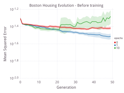
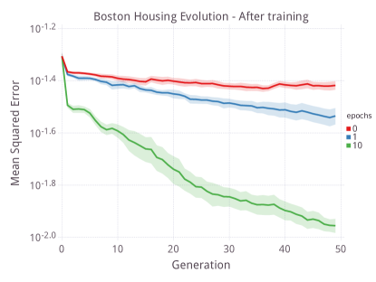
Figure 3: GRN evolution using different epochs for fitness. The baseline evolution is indicated as 0 training epochs. On the left is MSE before training; on the right is MSE after training. Ribbons indicate one standard deviation over 10 trials.

4 Results

Overall, the results demonstrate that evolution can allow learning to reach more optimal points in the search space that elude learning when performed on random GRNs. Together, learning and evolution reach similar performance to fully converged learners.

Figure 3 shows the MSE of the best individuals from each evolution, before and after training. Evolution with 10 epochs of training shows that using trained MSE as evolutionary fitness starts to constitute a different evolutionary task. The error of GRNs before training in this evolution converges above evolution-only. However, the decreasing trained error shows that evolution is improving these GRNs. Instead of improving initial fitness on the regression task, the learning capability, or “learnability”, of the population is increased over time.

Finally, we compare the trained GRNs from the 10 epoch evolution to other models. The GRN performs better than an RNN layer of the same size, and better than some trials of a dense neural network. An interesting comparison is the random GRN with 50 regulatory proteins and the dense layer, which has 60 hidden nodes. Both have a wide distribution based on initial conditions, but are capable of very good error results. This again demonstrates the importance of initialization for learning.

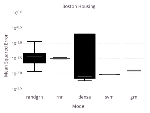
Figure 4: Test MSE of the best GRNs from the 10 epoch evolution and of other trained models

5 Discussion

In this work, we have demonstrated that a differentiable GRN can be used as a layer in a learning model. While learning was only performed on individual layers in this work, the Keras GRN layer can easily be used in conjunction with other layer types. We believe this model is one of the first successful implementations of an evolutionary layer in a modern deep learning framework, and can provide an alternative to RNN layers. We are also interested in understanding the capabilities of models with multiple GRN layers, stacked similarly to deep neural network layers.

This work also explored the complex relationship between learning and evolution. The Baldwin Effect is not a well-understood phenomena for artificial evolution, and there are many open questions related to it. In this work, we chose constant training periods for simplicity, but observed cases where learning was unnecessary for certain individuals, or where more learning could be beneficial. An automatic process could instead determine the length of training for each individual, or each generation. Understanding how such a process impacts the Baldwin Effect is intended as future work.

Also for the sake of simplicity, this work used the same evolutionary fitness for the baseline evolution and evolution with learning. This may result in overfitting on the training set used in evolution. Instead, one could use a validation score as the evolutionary fitness for learning runs. This opens the broader question of designing evolutionary goals specifically for learning individuals. Metrics to measure the learning capacity, such as the average increase over epoch, could be used. The results demonstrate that such a fitness measure may be used implicitly by evolution, but a designed metric for learning may be even more effective.

Finally, the GRN benefits from having an evolvable encoding which is also now differentiable, with no mapping from genotype to phenotype for learning. This means the learned weights can be directly returned to the genome in a Lamarckian evolution scheme. Preliminary results with Lamarckian evolution demonstrate that this is a powerful search mechanism and the use of the GRN model in Lamarckian evolution will be the topic of future study.

Acknowledgments

This work is supported by ANR-11-LABX-0040-CIMI, within programme ANR-11-IDEX-0002-02.

References

- [Ancel, 2000] Ancel, L. W. (2000). Undermining the baldwin expediting effect: does phenotypic plasticity accelerate evolution? Theoretical population biology, 58(4):307–319.
- [Ancel et al., 2000] Ancel, L. W., Fontana, W., et al. (2000). Plasticity, evolvability, and modularity in rna. Journal of Experimental Zoology, 288(3):242–283.
- [Baldwin, 1896] Baldwin, J. M. (1896). A new factor in evolution. The american naturalist, 30(354):441–451.
- [Banzhaf, 2003] Banzhaf, W. (2003). Artificial regulatory networks and genetic programming. In Genetic programming theory and practice, pages 43–61. Springer.
- [Cussat-Blanc and Harrington, 2015] Cussat-Blanc, S. and Harrington, K. (2015). Genetically-regulated Neuromodulation Facilitates Multi-Task Reinforcement Learning. In Proceedings of the 2015 on Genetic and Evolutionary Computation Conference - GECCO ’15, number 1, pages 551–558, New York, New York, USA. ACM Press.
- [Cussat-Blanc et al., 2015] Cussat-Blanc, S., Harrington, K., and Pollack, J. (2015). Gene Regulatory Network Evolution Through Augmenting Topologies. IEEE Transactions on Evolutionary Computation, 19(6):823–837.
- [Cussat-Blanc et al., 2008] Cussat-Blanc, S., Luga, H., and Duthen, Y. (2008). From single cell to simple creature morphology and metabolism. Artificial Life XI, pages 134–141.
- [Disset et al., 2017] Disset, J., Wilson, D. G., Cussat-Blanc, S., Sanchez, S., Luga, H., and Duthen, Y. (2017). A comparison of genetic regulatory network dynamics and encoding. In Proceedings of the Genetic and Evolutionary Computation Conference, pages 91–98. ACM.
- [Fernando et al., 2016] Fernando, C., Banarse, D., Reynolds, M., Besse, F., Pfau, D., Jaderberg, M., Lanctot, M., and Wierstra, D. (2016). Convolution by evolution: Differentiable pattern producing networks. In Proceedings of the Genetic and Evolutionary Computation Conference 2016, pages 109–116. ACM.
- [Hinton and Nowlan, 1987] Hinton, G. E. and Nowlan, S. J. (1987). How learning can guide evolution. Complex systems, 1(3):495–502.
- [Joachimczak and Wrobel, 2010] Joachimczak, M. and Wrobel, B. (2010). Evolving Gene Regulatory Networks for Real Time Control of Foraging Behaviours. Artificial Life XII. Proceedings of the 12th International Conference on the Synthesis and Simulation of Living Systems, pages 348–355.
- [Joachimczak and Wróbel, 2010] Joachimczak, M. and Wróbel, B. b. (2010). Processing signals with evolving artificial gene regulatory networks. Artificial Life XII: Proceedings of the 12th International Conference on the Synthesis and Simulation of Living Systems, ALIFE 2010, pages 203–210.
- [Kingma and Ba, 2014] Kingma, D. P. and Ba, J. (2014). Adam: A method for stochastic optimization. arXiv preprint arXiv:1412.6980.
- [Kuo et al., 2004] Kuo, P. D., Leier, A., and Banzhaf, W. (2004). Evolving dynamics in an artificial regulatory network model. In International Conference on Parallel Problem Solving from Nature, pages 571–580. Springer.
- [Lipson et al., 2002] Lipson, H., Pollack, J. B., and Suh, N. P. (2002). On the origin of modular variation. Evolution, 56(8):1549–1556.
- [Rohlf and Winkler, 2009] Rohlf, T. and Winkler, C. R. (2009). Emergent network structure, evolvable robustness, and nonlinear effects of point mutations in an artificial genome model. Advances in Complex Systems, 12:293–310.
- [Schemmel et al., 2006] Schemmel, J., Grubl, A., Meier, K., and Mueller, E. (2006). Implementing synaptic plasticity in a vlsi spiking neural network model. In Neural Networks, 2006. IJCNN’06. International Joint Conference on, pages 1–6. IEEE.
- [Schramm et al., 2012] Schramm, L., Jin, Y., and Sendhoff, B. (2012). Redundancy in the evolution of artificial gene regulatory networks for morphological development. In IEEE Symposium on Computational Intelligence in Bioinformatics and Computational Biology.
- [Wilson et al., 2013] Wilson, D., Awa, E., Cussat-Blanc, S., Veeramachaneni, K., and O’Reilly, U.-M. (2013). On learning to generate wind farm layouts. Fifteenth annual conference on Genetic and evolutionary computation conference, pages 767–774.
- [Wróbel and Abdelmotaleb, 2012] Wróbel, B. and Abdelmotaleb, A. (2012). Evolving Spiking Neural Networks in the GReaNs ( Gene Regulatory evolving artificial Networks ) Plaftorm. EvoNet2012: Evolving Networks, from Systems/Synthetic Biology to Computational Neuroscience Workshop at Artificial Life XIII, pages 19–22.