Massive three loop form factors in the planar limit

Abstract:

We present the color planar and complete light quark QCD contributions to the three loop heavy quark form factors in the case of vector, axial-vector, scalar and pseudo-scalar currents. We evaluate the master integrals applying a new method based on differential equations for general bases, which is applicable for any first order factorizing systems. The analytic results are expressed in terms of harmonic polylogarithms and real-valued cyclotomic harmonic polylogarithms.

1 Introduction

The top quark, being the heaviest particle of the Standard Model (SM), plays a significant role in understanding the electro-weak symmetry breaking (EWSB). Besides, its heftiness generates a strong potential for hidden beyond the SM (BSM) physics scenarios. Hence, a detailed study on top quark observables is always a crucial topic. On the other hand, the abundance of top quark pair production at the high energy colliders allows us to obtain accurate measurements. Especially at the future linear or circular electron-positron colliders, the experimental accuracy for this channel will reach ultimate precision. In order to match the experimental accuracy, precise predictions are required on the theoretical side as well. Perturbative quantum chromodynamics (QCD) effects constitute the major contributions in precision physics and one of the main ingredients of QCD corrections is the form factor. Form factors are the matrix elements of local composite operators between physical states. In scattering cross-sections, they provide important contributions to the virtual corrections. The vector and axial-vector massive form factors are of importance for the forward-backward asymmetry of bottom or top quark pair production at electron-positron colliders while, the scalar and pseudo-scalar ones may shed light on the decay of a Higgs boson to a pair of heavy quarks. They are also important to inspect the properties of the top quark [1, 2] during the high luminosity phase of the LHC [3] and the experimental precision studies at future high energy $e^{+}e^{-}$ colliders [4].

In this note, we present both the color–planar and complete light quark non-singlet three-loop contributions to the massive form factors for vector, axial-vector, scalar and pseudo-scalar currents. Our results except for the vector current, are presented in [5] and for the vector current, including the technical details, will be presented elsewhere [6]. In [7, 8, 9, 10], the two-loop QCD corrections to the massive vector, axial-vector form factors, the anomaly contributions, and the scalar and pseudo-scalar form factors were first presented. In [11], an independent computation led to a cross-check of the vector form factor, including the additional ${\mathcal{O}}(\varepsilon)$ terms in the dimensional parameter $\varepsilon=(4-D)/2$. The contributions up to ${\mathcal{O}}(\varepsilon^{2})$ for all the massive two-loop form factors were obtained recently in Ref. [12]. The color–planar contributions to the massive three-loop vector form factor have been computed in [13, 14] and the complete light quark contributions in [15]. In a parallel and independent computation in [16], the authors also have obtained both the color–planar and complete light quark non-singlet three-loop massive form factors for the aforementioned currents. In [17], the large $\beta_{0}$ limit has been considered.

2 Notation

The notations follow those used in Ref. [5, 12]. To summarize, we consider the decay of a virtual massive boson of momentum $q$ into a pair of heavy quarks of mass $m$, momenta $q_{1}$ and $q_{2}$ and color $c$ and $d$, through a vertex indicated by $I=V,A,S,P$ for a vector, an axial-vector, a scalar and a pseudo-scalar boson, respectively. Here $q^{2}=(q_{1}+q_{2})^{2}$ is the center of mass energy squared and the dimensionless variable $s$ is defined by

$$s=\frac{q^{2}}{m^{2}}\,.$$ (1)

By studying the Lorentz structure, the following general form of the amplitudes for the vector and axial-vector currents can be obtained

$$-i\delta_{cd}~{}\bar{u}_{c}(q_{1})~{}\Big{[}v_{Q}\Big{(}\gamma^{\mu}~{}F_{V,1}+\frac{i}{2m}\sigma^{\mu\nu}q_{\nu}~{}F_{V,2}\Big{)}+a_{Q}\Big{(}\gamma^{\mu}\gamma_{5}~{}F_{A,1}+\frac{1}{2m}q^{\mu}\gamma_{5}~{}F_{A,2}\Big{)}\Big{]}~{}v_{d}(q_{2}),$$ (2)

and for the scalar and pseudo-scalar currents

$$-\frac{m}{v}\delta_{cd}~{}\bar{u}_{c}(q_{1})~{}\Big{[}s_{Q}\,F_{S}+ip_{Q}\gamma_{5}\,F_{P}\Big{]}~{}v_{d}(q_{2})\,.$$ (3)

$\bar{u}_{c}(q_{1})$ and $v_{d}(q_{2})$ are the bi-spinors of the quark and the anti-quark, respectively. The scalar objects, $F_{I}$, with $I=V,A,S,P$, are the corresponding form factors, expanded in the strong coupling constant $\alpha_{s}=g_{s}^{2}/(4\pi)$ as follows

$$F_{I}=\sum_{n=0}^{\infty}\left(\frac{\alpha_{s}}{4\pi}\right)^{n}F_{I}^{(n)}\,.$$ (4)

$\sigma^{\mu\nu}=\frac{i}{2}[\gamma^{\mu},\gamma^{\nu}]$ and $v_{Q},a_{Q},s_{Q},p_{Q}$ are the vector, axial-vector, scalar and pseudo-scalar coupling constant, respectively. $v=(\sqrt{2}G_{F})^{-1/2}$ is the SM vacuum expectation value of the Higgs field, with $G_{F}$ being the Fermi constant. Finally, we multiply appropriate projectors as provided in [12], to obtain the unrenormalized form factors. Next, the trace over the color and spinor indices is performed. For later purposes we denote the number of colors by $N_{c}$. $n_{l}$ and $n_{h}$ are the number of light and heavy quarks, respectively.

Since we use dimensional regularization [18], the important factor for axial-vector and pseudo-scalar currents, is a proper definition of $\gamma_{5}$ in $D$ space-time dimensions. As both the color-planar and complete light quark contributions belong to the so-called non-singlet case, where the axial-vector or pseudo-scalar vertex is connected to open heavy quark lines, both $\gamma_{5}$-matrices appear in the same chain of Dirac matrices. Hence we can conveniently use an anti-commuting $\gamma_{5}$ in $D$ space-time dimensions, with $\gamma_{5}^{2}=1$. This also implies the well-known Ward identity,

$$q^{\mu}\Gamma_{A,cd}^{\mu,\sf ns}=2m\Gamma_{P,cd}^{\sf ns}\,,$$ (5)

which in terms of the form factors, takes the following form

$$2F_{A,1}^{\sf ns}+\frac{s}{2}F_{A,2}^{\sf ns}=2F_{P}^{\sf ns}\,.$$ (6)

Here, the non-singlet contributions are denoted by ${\sf ns}$. For convenience, we introduce the Landau variable [19]

$$x=\frac{\sqrt{q^{2}-4m^{2}}-\sqrt{q^{2}}}{\sqrt{q^{2}-4m^{2}}+\sqrt{q^{2}}}\quad\leftrightarrow\quad s=\frac{q^{2}}{m^{2}}=-\frac{(1-x)^{2}}{x}.$$ (7)

3 Computational details

We follow the generic procedure to compute the form factors. The Feynman diagrams are generated using QGRAF [20]. The QGRAF output is then processed using Q2e/Exp [21, 22] and FORM [23, 24]. The color algebra has been performed using Color [25]. By decomposing the dot products among the loop and external momenta, the diagrams can be expressed in terms of a linear combination of a large set of scalar integrals.

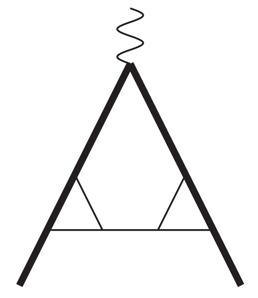
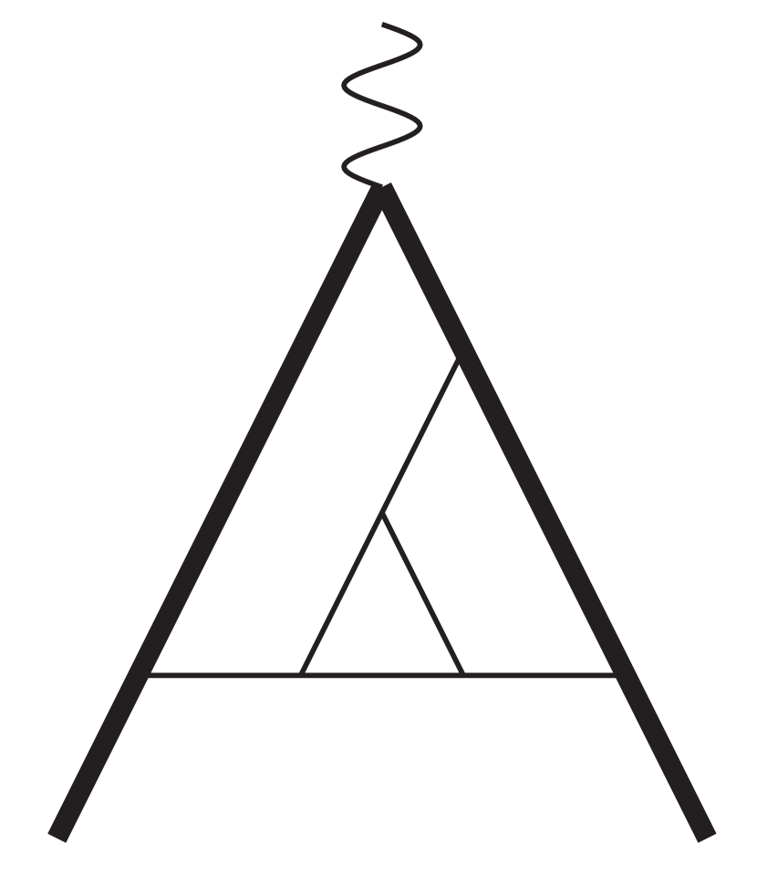
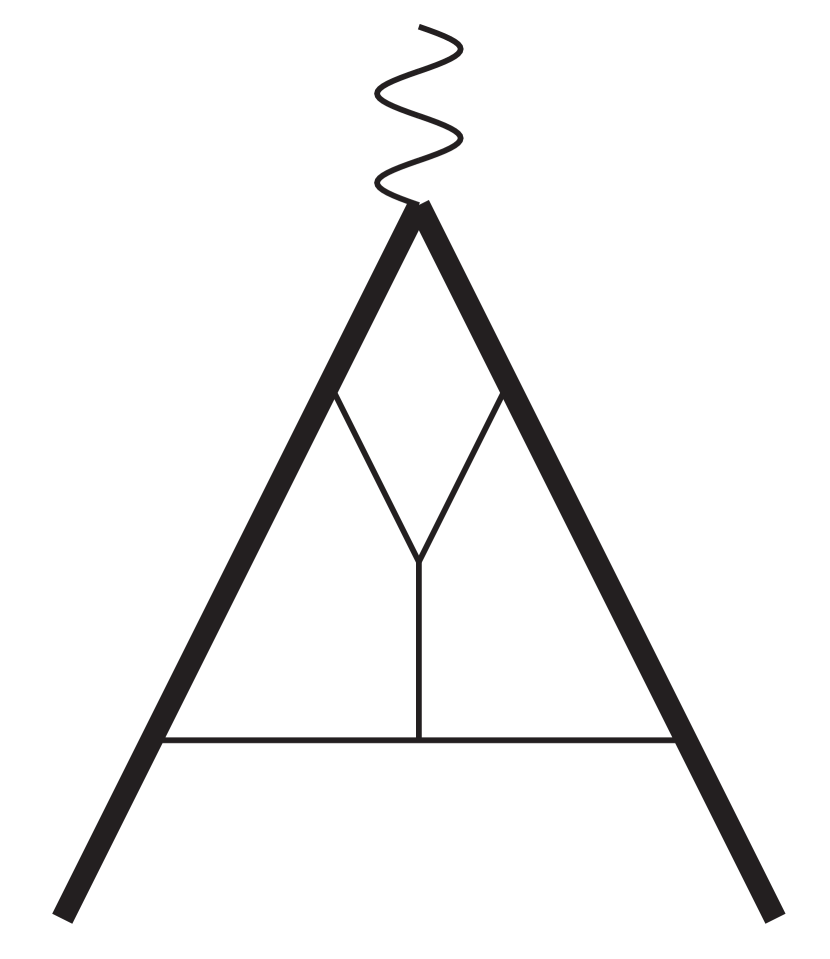
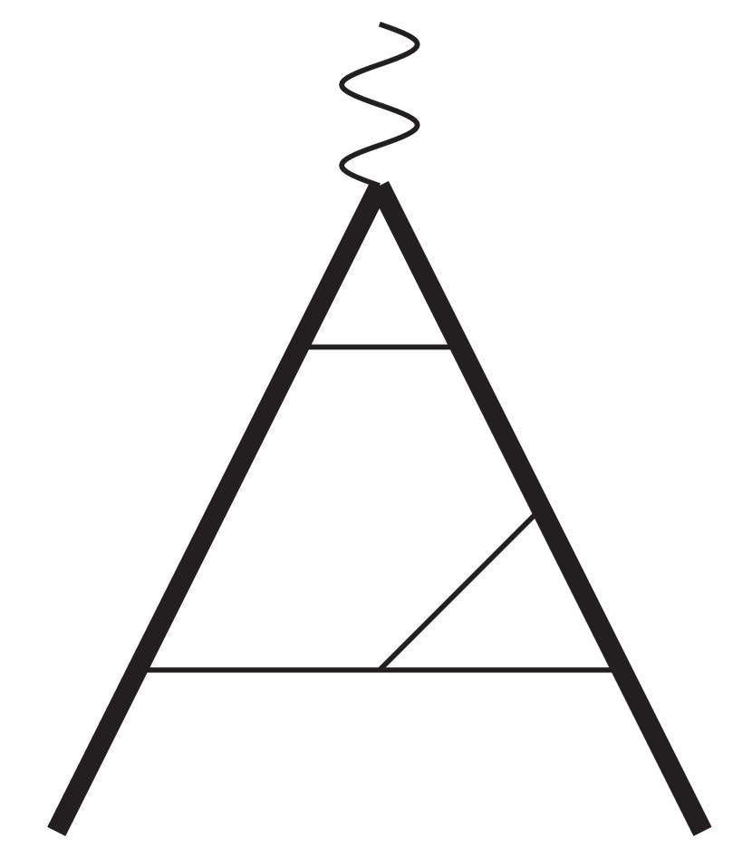
Figure 1: The color-planar topologies

These integrals are then reduced using integration by parts identities (IBPs) [26, 27] with the help of the program Crusher [28] to obtain 109 master integrals (MIs), out of which 96 appear in the color-planar case. In the color-planar limit, the families of integrals can be represented by eight topologies, shown in Figure 1, whereas for the complete light quark contributions, three more topologies, cf. Figure 2, are required .

Figure 2: The $n_{l}$ topologies

Finally, to compute the MIs, we use the method of differential equations [29, 30, 31, 32]. For a recent review on the computational methods of loop integrals in quantum field theory, see [33]. The basic idea is to obtain a set of differential equations of the MIs by performing differentiation w.r.t $x$ and then to use the IBP relations. The first step to solve the corresponding linear system of differential equations is to find out whether the system is first order factorizable or not. Using the package Oresys [34], based on Zürcher’s algorithm [35, 36], we have found that the present system is indeed first order factorizable in $x$-space. Without any need to choose a special basis, we can now simply solve the system in terms of iterated integrals of whatsoever alphabet, cf. Ref. [6] for details. The differential equations are solved order by order in $\varepsilon$ successively, starting at the leading pole terms $\propto 1/\varepsilon^{3}$. The successive solutions in $\varepsilon$ contribute to the inhomogeneities in the next order. We compute the master integrals block-by-block, where for an $m\times m$ system, $l$ single inhomogeneous ordinary differential equations are obtained, where $1\leq l\leq m$. The orders of these differential equations are $m_{1},\ldots,m_{l}$ such that $m_{1}+\cdots+m_{l}=m$. We have solved these differential equations using the variation of constant. The other $m-l$ solutions result from the former solution immediately. The constants of integration are determined using boundary conditions at $x=1$. The calculation is performed by intense use of HarmonicSums [37, 38, 39, 40, 41, 42, 43], which uses the package Sigma [44, 45]. Finally, all the MIs have been checked numerically using FIESTA [46, 47, 48].

The non-homogeneous contributions contain only rational functions of $x$ and hence the results can be written in terms of iterative integrals. While integration over a letter is a straightforward algebraic manipulation, often $k$-th powers of a letter, $k\in\mathbb{N}$, appear which needs to be transformed to the letter by partial integration. This method is partially related to the method of hyperlogarithms [49, 50]. We obtain up to weight w=6 real-valued iterated integrals over the alphabet

$$\frac{1}{x},~{}~{}\frac{1}{1-x},~{}~{}\frac{1}{1+x},~{}~{}\frac{1}{1-x+x^{2}},~{}~{}\frac{x}{1-x+x^{2}},$$ (8)

i.e. the usual harmonic polylogarithms (HPLs) [51] and their cyclotomic extension [37], including the respective constants in the limit $x\rightarrow 1$, i.e. the multiple zeta values (MZVs) [52] and the cyclotomic constants [37, 53, 54]. The use of shuffle algebra [55], implemented in HarmonicSums, reduces the number of functions accordingly, which facilitates numerical evaluation. In the MZVs and cyclotomic cases, there are proven reduction relations to weight w = 12 [52] and w = 6 [53, 54], respectively, which have been used. The 188 cyclotomic constants which appear up to w = 6, reduce to 23 constants. Note that there are more conjectured relations, cf. [56], based on PSLQ [57]. If these conjectured relations are used, only MZVs remain as constants in all form factors. The analytic result for the different form factors in terms of HPLs and cyclotomic HPLs [51, 37] can be analytically continued outside $x~{}\in~{}[0,1[$ by using the mappings $x\rightarrow-x,x\rightarrow(1-x)/(1+x)$ on the expense of extending the cyclotomy class in cases needed.

4 Ultraviolet renormalization and universal infrared structure

To perform the ultraviolet (UV) renormalization of the form factors, we choose a mixed scheme. The heavy quark mass and wave function have been renormalized in the on-shell (OS) renormalization scheme. We renormalize the strong coupling constant in the $\overline{\rm MS}$ scheme, by setting the universal factor $S_{\varepsilon}=\exp(-\varepsilon(\gamma_{E}-\ln(4\pi))$ for each loop order to one at the end of the calculation. The required renormalization constants are already well known and denoted by $Z_{m,{\rm OS}}$ [58, 59, 60, 61, 62], $Z_{2,{\rm OS}}$ [58, 59, 60, 63] and $Z_{a_{s}}$ [64, 65] for the heavy quark mass, wave function and strong coupling constant, respectively. For all the currents, the renormalization of the heavy-quark wave function and the strong coupling constant are multiplicative, while the renormalization of massive fermion lines has been taken care of by properly considering the counter terms. For the scalar and pseudo-scalar currents, presence of the heavy quark mass in the Yukawa coupling employs another overall mass renormalization constant, which also has been performed in OS renormalization scheme.

The universal behavior of infrared (IR) singularities of the massive form factors was first investigated in [66] considering the high energy limit. Later in [67], a general argument was provided to factorize the IR singularities as a multiplicative renormalization constant. Its structure is constrained by the renormalization group equation (RGE), as follows,

$$F_{I}=Z(\mu)F_{I}^{\mathrm{fin}}(\mu)\,,$$ (9)

where $F_{I}^{\mathrm{fin}}$ is finite as $\varepsilon\rightarrow 0$. The RGE for $Z(\mu)$ reads

$$\frac{d}{d\ln\mu}\ln Z(\varepsilon,x,m,\mu)=-\Gamma(x,m,\mu)\,,$$ (10)

where $\Gamma$ is the corresponding cusp anomalous dimension, which is by now available up to three-loop order [68, 69]. Notice that $Z$ does not carry any information regarding the vertex. Both $Z$ and $\Gamma$ can be expanded in a perturbative series in $\alpha_{s}$ as follows

$$Z=\sum_{n=0}^{\infty}\left(\frac{\alpha_{s}}{4\pi}\right)^{n}Z^{(n)}\,,\qquad\Gamma=\sum_{n=0}^{\infty}\left(\frac{\alpha_{s}}{4\pi}\right)^{n+1}\Gamma_{n}$$ (11)

and one finds the following solution for Eq. (10)

$$Z =1+\left(\frac{\alpha_{s}}{4\pi}\right)\Bigg{[}\frac{\Gamma_{0}}{2\varepsilon}\Bigg{]}+\left(\frac{\alpha_{s}}{4\pi}\right)^{2}\Bigg{[}\frac{1}{\varepsilon^{2}}\Big{(}\frac{\Gamma_{0}^{2}}{8}-\frac{\beta_{0}\Gamma_{0}}{4}\Big{)}+\frac{\Gamma_{1}}{4\varepsilon}\Bigg{]}$$

$$+\left(\frac{\alpha_{s}}{4\pi}\right)^{3}\bigg{[}\frac{1}{\varepsilon^{3}}\left(\frac{\Gamma_{0}^{3}}{48}-\frac{\beta_{0}\Gamma_{0}^{2}}{8}+\frac{\beta_{0}^{2}\Gamma_{0}}{6}\right)+\frac{1}{\varepsilon^{2}}\left(\frac{\Gamma_{0}\Gamma_{1}}{8}-\frac{\beta_{1}\Gamma_{0}}{6}\right)+\frac{1}{\varepsilon}\left(\frac{\Gamma_{2}}{6}\right)\bigg{]}+{\cal O}(\alpha_{s}^{4})\,.$$ (12)

Eq. (4) correctly predicts the IR singularities for all massive form factors at the three-loop level.

5 Results and checks

We finally obtain the color–planar and the complete light quark non–singlet ($n_{l}$) contributions for the three-loop massive form factors for vector, axial-vector, scalar and pseudo-scalar currents. The expressions, except for the vector current, are attached as supplemental material along with the publication [5]. The corresponding results for vector current will be available in [6].

Figure 3: The $O(\varepsilon^{0})$ contribution to the vector three-loop form factors $F_{V,1}^{(3)}$ (left) and $F_{V,2}^{(3)}$ (right) as a function of $x$. Dash-dotted line: leading color contribution of the non-singlet form factor; Full line: sum of the complete non-singlet $n_{l}$-contributions for $n_{l}=5$ and the color-planar non-singlet form factor; Dashed line: large $x$ expansion; Dotted line: small $x$ expansion.

Figure 4: The $O(\varepsilon^{0})$ contribution to the axial-vector three-loop form factors $F_{A,1}^{(3)}$ (left) and $F_{A,2}^{(3)}$ (right) as a function of $x$. Dash-dotted line: leading color contribution of the non-singlet form factor; Full line: sum of the complete non-singlet $n_{l}$-contributions for $n_{l}=5$ and the color-planar non-singlet form factor; Dashed line: large $x$ expansion; Dotted line: small $x$ expansion.

In Figures 3–5 we illustrate the behaviour of the $O(\varepsilon^{0})$ parts of the different form factors as a function of $x\in[0,1]$. We also show their small- and large-$x$ expansions. The latter representations are obtained using HarmonicSums. The different limits are characterized as follows :

Low energy region ($x\rightarrow 1$): In the space-like case ($q^{2}<0$) we have expanded the form factors, redefining $x=e^{i\phi}$, $\phi=0$.

High energy region ($x\rightarrow 0$): Here we expand the form factors up to ${\cal O}(x^{4})$. The chirality flipping form factors $F_{V,2}$ and $F_{A,2}$ vanish and the effect of $\gamma_{5}$ gets nullified in this limit implying $F_{V,1}=F_{A,1}$ and $F_{S}=F_{P}$. In the small quark mass limit, the form factors satisfy the Sudakov evolution equation. A detailed study has been performed in [66, 70] to predict part of the vector form factors in this limit from the then available components up to three and four loop level, respectively.

Threshold region ($x\rightarrow-1$): We define $\beta=\sqrt{1-\frac{4m^{2}}{q^{2}}}$ and expand the form factors around $\beta=0$.

For the numerical evaluation of the HPLs and cyclotomic HPLs in the Kummer representation, we use the GiNaC-package [71, 72].

Figure 5: The $O(\varepsilon^{0})$ contribution to the scalar and pseudo-scalar three-loop form factors $F_{S}^{(3)}$ (left) and $F_{P}^{(3)}$ (right) as a function of $x$. Dash-dotted line: leading color contribution of the non-singlet form factor; Full line: sum of the complete non-singlet $n_{l}$-contributions for $n_{l}=5$ and the color-planar non-singlet form factor; Dashed line: large $x$ expansion; Dotted line: small $x$ expansion.

We have performed a series of further checks. Through an explicit computation, the Ward identity Eq. (6) has been checked. By maintaining the gauge parameter $\xi$ to first order throughout the calculation, a partial check on gauge invariance has been achieved. After $\alpha_{s}$-decoupling, the UV renormalized results satisfy the universal IR structure, confirming again the correctness of all pole terms. Finally, we have compared our results with those of Ref. [16], which has been obtained using different methods, and agree by adjusting the respective conventions.

Acknowledgment.  This work was supported in part by the Austrian Science Fund (FWF) grant SFB F50 (F5009-N15). We would like to thank M. Steinhauser for providing their yet unpublished results in electronic form and A. De Freitas and V. Ravindran for discussions. The Feynman diagrams have been drawn using Axodraw [73].

References

- [1] F. Abe et al. [CDF Collaboration], Phys. Rev. Lett. 74 (1995) 2626–2631 [hep-ex/9503002].
- [2] S. Abachi et al. [D0 Collaboration], Phys. Rev. Lett. 74 (1995) 2632–2637 [hep-ex/9503003].
- [3] https://home.cern/topics/high-luminosity-lhc
- [4] E. Accomando et al. [ECFA/DESY LC Physics Working Group], Phys. Rept. 299 (1998) 1 [hep-ph/9705442].
- [5] J. Ablinger, J. Blümlein, P. Marquard, N. Rana and C. Schneider, Phys. Lett. B 782 (2018) 528 [arXiv:1804.07313 [hep-ph]].
- [6] J. Ablinger, J. Blümlein, P. Marquard, N. Rana, and C. Schneider, DESY 18-053, DO-TH 18/09.
- [7] W. Bernreuther, R. Bonciani, T. Gehrmann, R. Heinesch, T. Leineweber, P. Mastrolia, and E. Remiddi, Nucl. Phys. B706 (2005) 245–324 [hep-ph/0406046].
- [8] W. Bernreuther, R. Bonciani, T. Gehrmann, R. Heinesch, T. Leineweber, P. Mastrolia, and E. Remiddi, Nucl. Phys. B712 (2005) 229–286 [hep-ph/0412259].
- [9] W. Bernreuther, R. Bonciani, T. Gehrmann, R. Heinesch, T. Leineweber, and E. Remiddi, Nucl. Phys. B723 (2005) 91–116 [hep-ph/0504190].
- [10] W. Bernreuther, R. Bonciani, T. Gehrmann, R. Heinesch, P. Mastrolia, and E. Remiddi, Phys. Rev. D72 (2005) 096002 [hep-ph/0508254].
- [11] J. Gluza, A. Mitov, S. Moch, and T. Riemann, JHEP 07 (2009) 001, [arXiv:0905.1137 [hep-ph]].
- [12] J. Ablinger, A. Behring, J. Blümlein, G. Falcioni, A. De Freitas, P. Marquard, N. Rana and C. Schneider, Phys. Rev. D 97 (2018) no.9, 094022 [arXiv:1712.09889 [hep-ph]].
- [13] J.M. Henn, A.V. Smirnov, V.A. Smirnov, and M. Steinhauser, JHEP 01 (2017) 074, [arXiv:1611.07535 [hep-ph]].
- [14] J.M. Henn, A.V. Smirnov, and V.A. Smirnov, JHEP 12 (2016) 144, [arXiv:1611.06523 [hep-ph]].
- [15] R.N. Lee, A.V. Smirnov, V.A. Smirnov and M. Steinhauser, JHEP 1803 (2018) 136 [arXiv:1801.08151 [hep-ph]].
- [16] R. N. Lee, A. V. Smirnov, V. A. Smirnov and M. Steinhauser, JHEP 1805 (2018) 187 [arXiv:1804.07310 [hep-ph]].
- [17] A. Grozin, Eur. Phys. J. C 77 (2017) no.7, 453 [arXiv:1704.07968 [hep-ph]].
- [18] G. ’t Hooft and M.J.G. Veltman, Nucl. Phys. B44 (1972) 189–213.
- [19] R. Barbieri, J. A. Mignaco, and E. Remiddi, Nuovo Cim. A11 (1972) 824–864; 865–916.
- [20] P. Nogueira, J. Comput. Phys. 105 (1993) 279–289.
- [21] R. Harlander, T. Seidensticker, and M. Steinhauser, Phys. Lett. B426 (1998) 125–132 [hep-ph/9712228].
- [22] T. Seidensticker, in: Proc. of the 6th International Workshop on New Computing Techniques in Physics Research (AIHENP 99) Heraklion, Crete, Greece, April 12-16, 1999, hep-ph/9905298.
- [23] J.A.M. Vermaseren, New features of FORM, math-ph/0010025.
- [24] M. Tentyukov and J.A.M. Vermaseren, Comput. Phys. Commun. 181 (2010) 1419–1427 [hep-ph/0702279].
- [25] T. van Ritbergen, A.N. Schellekens and J.A.M. Vermaseren, Int. J. Mod. Phys. A 14 (1999) 41 [hep-ph/9802376].
- [26] K.G. Chetyrkin and F.V. Tkachov, Nucl. Phys. B 192 (1981) 159.
- [27] S. Laporta, Int. J. Mod. Phys. A 15 (2000) 5087 [hep-ph/0102033].
- [28] P. Marquard and D. Seidel, The package Crusher, (unpublished).
- [29] A.V. Kotikov, Phys. Lett. B254 (1991) 158–164.
- [30] E. Remiddi, Nuovo Cim. A110 (1997) 1435–1452 [hep-th/9711188].
- [31] J.M. Henn, Phys. Rev. Lett. 110 (2013) 251601 [arXiv:1304.1806 [hep-th]].
- [32] J. Ablinger, A. Behring, J. Blümlein, A. De Freitas, A. von Manteuffel and C. Schneider, Comput. Phys. Commun. 202 (2016) 33–112 [arXiv:1509.08324 [hep-ph]].
- [33] J. Blümlein and C. Schneider, Int. J. Mod. Phys. A 33 (2018) no.17, 1830015.
- [34] S. Gerhold, Uncoupling systems of linear Ore operator equations, Master’s thesis, RISC, J. Kepler University, Linz, 2002.
- [35] B. Zürcher, Rationale Normalformen von pseudo-linearen Abbildungen, Master’s thesis, Mathematik, ETH Zürich (1994).
- [36] C. Schneider, A. De Freitas and J. Blümlein, PoS (LL2014) 017 [arXiv:1407.2537 [cs.SC]].
- [37] J. Ablinger, J. Blümlein, and C. Schneider, J. Math. Phys. 52 (2011) 102301 [arXiv:1105.6063 [math-ph]].
-
[38]
J.A.M. Vermaseren,
Int. J. Mod. Phys. A 14 (1999) 2037–2076
[hep-ph/9806280];
J. Blümlein and S. Kurth, Phys. Rev. D 60 (1999) 014018 [hep-ph/9810241]. - [39] J. Ablinger, PoS (LL2014) 019 [arXiv:1407.6180 [cs.SC]].
- [40] J. Ablinger, A Computer Algebra Toolbox for Harmonic Sums Related to Particle Physics. Master thesis, Linz U., 2009. arXiv:1011.1176 [math-ph].
- [41] J. Ablinger, Computer Algebra Algorithms for Special Functions in Particle Physics. PhD thesis, Linz U., 2012. arXiv:1305.0687 [math-ph].
- [42] J. Ablinger, J. Blümlein, and C. Schneider, J. Math. Phys. 54 (2013) 082301 [arXiv:1302.0378 [math-ph]].
- [43] J. Ablinger, J. Blümlein, C. G. Raab, and C. Schneider, J. Math. Phys. 55 (2014) 112301 [arXiv:1407.1822 [hep-th]].
- [44] C. Schneider, Sém. Lothar. Combin., 56 (2007), article B56b, 1–36.
- [45] C. Schneider, in: Computer Algebra in Quantum Field Theory: Integration, Summation and Special Functions, Eds. C. Schneider and J. Blümlein, (Springer, Wien, 2013), pp. 325–360, [arXiv:1304.4134 [cs.SC]].
- [46] A.V. Smirnov and M.N. Tentyukov, Comput. Phys. Commun. 180 (2009) 735 [arXiv:0807.4129 [hep-ph]].
- [47] A.V. Smirnov, V.A. Smirnov and M. Tentyukov, Comput. Phys. Commun. 182 (2011) 790 [arXiv:0912.0158 [hep-ph]].
- [48] A.V. Smirnov, Comput. Phys. Commun. 204 (2016) 189 [arXiv:1511.03614 [hep-ph]].
- [49] F. Brown, Commun. Math. Phys. 287 (2009) 925 [arXiv:0804.1660 [math.AG]].
- [50] J. Ablinger, J. Blümlein, C. Raab, C. Schneider and F. Wißbrock, Nucl. Phys. B 885 (2014) 409 [arXiv:1403.1137 [hep-ph]].
- [51] E. Remiddi and J.A.M. Vermaseren, Int. J. Mod. Phys. A15 (2000) 725–754 [hep-ph/9905237].
- [52] J. Blümlein, D.J. Broadhurst and J.A.M. Vermaseren, Comput. Phys. Commun. 181 (2010) 582 [arXiv:0907.2557 [math-ph]].
- [53] J. Ablinger, J. Blümlein, M. Round and C. Schneider, PoS (RADCOR2017) 010 [arXiv: 1712.08541 [hep-th]].
- [54] J. Ablinger, J. Blümlein, and C. Schneider, in preparation.
- [55] J. Blümlein, Comput. Phys. Commun. 159 (2004) 19 [hep-ph/0311046].
- [56] J.M. Henn, A.V. Smirnov and V.A. Smirnov, Nucl. Phys. B 919 (2017) 315 [arXiv:1512.08389 [hep-th]].
- [57] H.R.P. Ferguson and D.H. Bailey, A Polynomial Time, Numerically Stable Integer Relation Algorithm, RNR Techn. Rept, RNR-91-032, Jul. 14, 1992.
- [58] D.J. Broadhurst, N. Gray, and K. Schilcher, Z. Phys. C52 (1991) 111–122.
- [59] K. Melnikov and T. van Ritbergen, Nucl. Phys. B591 (2000) 515–546, [hep-ph/0005131].
- [60] P. Marquard, L. Mihaila, J.H. Piclum, and M. Steinhauser, Nucl. Phys. B773 (2007) 1–18 [arXiv:hep-ph/0702185 [hep-ph]].
- [61] P. Marquard, A.V. Smirnov, V.A. Smirnov and M. Steinhauser, Phys. Rev. Lett. 114 (2015) no.14, 142002 [arXiv:1502.01030 [hep-ph]].
- [62] P. Marquard, A.V. Smirnov, V.A. Smirnov, M. Steinhauser and D. Wellmann, Phys. Rev. D 94 (2016) no.7, 074025 [arXiv:1606.06754 [hep-ph]].
- [63] P. Marquard, A.V. Smirnov, V.A. Smirnov and M. Steinhauser, Phys. Rev. D 97 (2018) no.5, 054032 [arXiv:1801.08292 [hep-ph]].
- [64] O.V. Tarasov, A.A. Vladimirov and A.Y. Zharkov, Phys. Lett. 93B (1980) 429.
- [65] S. A. Larin and J. A. M. Vermaseren, Phys. Lett. B 303 (1993) 334 [hep-ph/9302208].
- [66] A. Mitov and S. Moch, JHEP 0705 (2007) 001 [hep-ph/0612149].
- [67] T. Becher and M. Neubert, Phys. Rev. D 79 (2009) 125004 Erratum: [Phys. Rev. D 80 (2009) 109901] [arXiv:0904.1021 [hep-ph]].
- [68] A. Grozin, J.M. Henn, G.P. Korchemsky, and P. Marquard, Phys. Rev. Lett. 114 no.~6, (2015) 062006 [arXiv:1409.0023 [hep-ph]].
- [69] A. Grozin, J.M. Henn, G.P. Korchemsky, and P. Marquard, JHEP 01 (2016) 140, [arXiv:1510.07803 [hep-ph]].
- [70] T. Ahmed, J. M. Henn and M. Steinhauser, JHEP 1706 (2017) 125 [arXiv:1704.07846 [hep-ph]].
- [71] J. Vollinga and S. Weinzierl, Comput. Phys. Commun. 167 (2005) 177 [hep-ph/0410259].
- [72] C. W. Bauer, A. Frink and R. Kreckel, J. Symb. Comput. 33 (2000) 1 [cs/0004015 [cs-sc]].
- [73] J.A.M. Vermaseren, Comput. Phys. Commun. 83 (1994) 45–58.