Comment on “Some exact quasinormal frequencies of a massless scalar field in Schwarzschild spacetime”

Abstract

A new branch of quasinormal modes for a massless scalar field propagating on the Schwarzschild spacetime was recently announced Batic et al. (2018). We review the quasinormal modes characterisation and arguments and identify the flaws in their proof. Then, we preset explicit counterexamples to such arguments. Finally, we study the modes via alternative methods and do not find the new branch. We conclude against their interpretation.

Introduction. Recently,Ref. Batic et al. (2018) announced a new branch of quasinormal modes (QNMs) for the scalar field on the Schwarzschild spacetime (see Chandrasekhar (1983); Kokkotas and Schmidt (1999); Nollert (1999); Berti et al. (2009); Konoplya and Zhidenko (2011) for main reviews). That study is based on Leaver’s work Leaver (1985). The approach deals with a $3$-term recurrence relation and the claimed QNMs correspond to values $s^{\rm new}_{k}\neq s^{\rm QNM}_{k}$ where one coefficient of the recurrence relation vanishes. In Ansorg and Panosso Macedo (2016); Panosso Macedo et al. (2018), Leaver’s approach is reinterpreted in the context of a hyperboloidal foliation of the spacetime and the algorithm is extended to discuss the spectral decomposition of the solution to the wave equation.

Here, we present the flaws in arguments in Ref. Batic et al. (2018), which are then identified in counterexamples. Specifically, the forward iteration of the recurrence relation leads to an exponential grow of the coefficients. While this growth agrees with the theoretical prediction, it contradicts a central assumption in the authors’ arguments that the sequence should decay. Complementarily, we calculate the QNMs as the eigenvalues of the operator associated to the wave equations and its boundary conditions and study its explicit time evolution. In neither of the alternatives approaches do we find the new frequencies.

Scalar field on Schwarzschild. The wave equation for a massless scalar field propagating on the Schwarzschild background reads (units $c=G=1$)

$$-f_{,\bar{t}\bar{t}}+f_{,xx}-{\cal P}f=0,$$ (1)

$${\cal P}=\left(\dfrac{2M}{r}\right)^{2}\left(1-\dfrac{2M}{r}\right)\left[\ell(\ell+1)+\dfrac{2M}{r}\right].$$ (2)

Here, $\bar{t}=t/(2M)$ and $x=r/(2M)+\ln\left[r/(2M)-1\right]$ are, respectively, the dimensionless time and tortoise coordinate.

We introduce Ansorg and Panosso Macedo (2016) the hyperboloidal coordinates $\{\tau,\sigma,\theta,\varphi\}$

$$t=2M\bigg{(}2\tau+\sigma^{-1}-\ln\left[\sigma(1-\sigma)\right]\bigg{)},\quad r=2M/\sigma.$$ (3)

The black-hole horizon ${\cal H}^{+}$ is at $\sigma=1$, whereas $\sigma=0$ locates future null infinity $\mathscr{I}^{+}$. The equation for $V(\tau,\sigma)=f(t(\tau,\sigma),r(\sigma))$ reads

$$-(1+\sigma)V_{,\tau\tau}+(1-2\sigma^{2})V_{,\tau\sigma}+\sigma^{2}(1-\sigma)V_{,\sigma\sigma}$$

$$+\sigma[2-3\sigma]V_{,\sigma}-2\sigma V_{,\tau}-[\ell(\ell+1)+\sigma]=0.$$ (4)

The regularity conditions at $\mathscr{I}^{+}$ and ${\cal H}^{+}$ account for the desired physical boundary conditions Ansorg and Panosso Macedo (2016); Panosso Macedo et al. (2018).

The Laplace transform of Eq. (Comment on “Some exact quasinormal frequencies of a massless scalar field in Schwarzschild spacetime”) yields ${\mathbf{A}}(s)\hat{V}(s)=B(s)$. The source term $B(s)$ contains the initial data Ansorg and Panosso Macedo (2016); Panosso Macedo et al. (2018), and

$${\mathbf{A}}(s)=\sigma^{2}(1-\sigma)\partial_{\sigma\sigma}+\left\{s(1-2\sigma^{2})+\sigma\left[2-3\sigma\right]\right\}\partial_{\sigma}$$

$$-\left[s^{2}(1+\sigma)+2\sigma\,s+\ell(\ell+1)+\sigma\right].$$ (5)

For the QNMs, we focus on the homogenous equation

$${\mathbf{A}}(s)\phi(s)=0.$$ (6)

This particular hyperboloidal foliation $\{\tau,\sigma\}$ is the spacetime counterpart of the analysis in Ref. Leaver (1985). Indeed, substituting

$$f(\bar{t},x)=e^{\bar{s}\bar{t}}F(x;\bar{s})$$ (7)

into (1), we obtain $F_{,xx}-\left[\bar{s}^{2}+{\cal P}\right]F=0,$ with $s=2\bar{s}.$ Ingoing/outgoing boundary conditions at infinity impose

$$F(x;\bar{s}) \sim e^{\mp\bar{s}x},\quad x\rightarrow\pm\infty.$$ (8)

While Leaver incorporates such asymptotics via Leaver (1985)

$$F(x(\sigma);\bar{s})=\Xi(\sigma;\bar{s})\,\phi(\sigma;2\bar{s}),\,\,\Xi(\sigma;\bar{s})=2e^{-\bar{s}/\sigma}\sigma^{\bar{s}}(1-\sigma)^{\bar{s}},$$ (9)

in Refs. Ansorg and Panosso Macedo (2016); Panosso Macedo et al. (2018), $\Xi(\sigma;\bar{s})$ follows directly from the substitution of (3) into (7). Finally, we expand $\phi(\sigma;s)$ in the Taylor series

$$\phi(\sigma;s)=\sum_{k=0}^{\infty}H_{k}(1-\sigma)^{k}.$$ (10)

Eq. (10) into (6) gives the $3$-term recurrence relation

$$\alpha_{k}H_{k+1}+\beta_{k}H_{k}+\gamma_{k}H_{k-1}=0\quad(k\geq 1),$$ (11)

with $\alpha_{k}=(k+1)(k+1+s),$ $-\beta_{k}=2(k+s)(k+1+s)+\ell(\ell+1)+1$ and $\gamma_{k}=(k+s)^{2}$.

Initial conditions. The initial seeds $H_{0}$ and $H_{1}$ for (11) must satisfy the initial condition

$$\alpha_{0}H_{1}+\beta_{0}H_{0}=0.\\$$ (12)

Equation (12) ensures the regularity of $\phi(\sigma;s)$ at $\sigma=1$, and it is equivalent to (11) at $k=0$ if and only if $H_{-1}=0$.

Proposition 1.

For any fixed $s\neq{\mathbb{Z}}^{-}$, there exists a unique (up to normalisation) sequence $\{H_{k}\}_{k=0}^{\infty}$ satisfying both (12) and (11). A convenient normalisation is $H_{0}=1$.

To construct $\{H_{k}\}_{k=0}^{\infty}$, one starts with $H_{0}=1$, then obtains $H_{1}=-\beta_{0}/\alpha_{0}$ according to (12), and finally calculates the remaining $H_{k}$ ($k\geq 1$) via a forward iteration of (11).

For a given exact value $s$, the forward iteration of Eqs. (12) and (11) is an exact calculation without any source numerical error. The technical limitation is restricted to a truncation $k=N_{\rm max}$ in the forward iteration procedure. From the practical perspective, one always deal with a finite sequence $\{H_{k}\}_{k=0}^{N_{\rm max}}$. For large $N_{\rm max}$, the values must be confronted against the asymptotic behaviours of the solutions to (11).

Asymptotic behavior. Equation (11) admits two independent asymptotic behaviours Batic et al. (2018); Ansorg and Panosso Macedo (2016)

$$H_{k,\pm}\sim k^{\zeta}\,e^{\pm\kappa\sqrt{k}}A_{k,\pm},\quad\Re(\kappa)>0,$$ (13)

$$\kappa=2\sqrt{s},\quad\zeta={s}/{2}-{3}/{4},\quad A_{k,\pm}=1+\sum\limits_{j=1}^{\infty}\dfrac{\mu_{\pm,i}}{k^{j/2}}.$$

Proposition 2.

For any fixed $s\neq{\mathbb{Z}}^{-}$ there exists unique (up to normalisation) sequences $\{H_{k,+}\}_{k=0}^{\infty}$ and $\{H_{k,-}\}_{k=0}^{\infty}$ satisfying (11) and the asymptotic behaviour (13). A convenient normalisation is $\displaystyle\lim_{k\rightarrow\infty}k^{-\zeta}e^{\mp\kappa\sqrt{k}}H_{k,\pm}=1$.

Thus, $\{H_{k}\}_{k=0}^{\infty}$ from Proposition (1) is a linear combination,

$$H_{k}=\lambda_{+}\,H_{k,+}+\lambda_{-}\,H_{k,-}.$$ (14)

Remark 1.

By imposing the initial seeds (12) at a given values $s$, a unique solution $\{H_{k}\}_{k=0}^{\infty}$ to  (11) is fixed. Thus, one does not have the freedom to choose a given asymptotic behaviour in the linear combination (14). In general, the exponential growth $H_{k}\sim e^{+\kappa\sqrt{k}}k^{\zeta}$ dominates for large $k$.

We are interested in the decaying solution $\{H_{k,-}\}_{k=0}^{\infty}$. While Proposition 2 is a formal result arising from an asymptotic study of Eq. (11), Refs. Ansorg and Panosso Macedo (2016); Panosso Macedo et al. (2018) discuss its explicit calculation (closely related to Leaver’s continued fraction Leaver (1985)). Briefly, one truncates the series at a given value $k=N_{\rm max}$ and approximates the values $H_{N_{\rm max},-}$ and $H_{N_{\rm max}-1,-}$ according to the behaviour (13). The complete sequence $\{H_{k,-}\}_{k=0}^{N_{\rm max}}$ is obtained by iterating (12) backwards up until $k=0$ Ansorg and Panosso Macedo (2016). The backward iteration provides us with $H_{-1,-}$ as well, which plays a crucial role when asserting the validity (12).

Remark 2.

By imposing the decaying asymptotic behaviour in (13) at a fixed values $s$, a unique solution $\{H_{k,-}\}_{k=0}^{\infty}$ to (11) is fixed. Thus, one does not have the freedom to impose the initial condition (12). In general, one obtains $H_{-1,-}\neq 0$.

At the QNMs $s^{\rm QNM}_{n}$ Leaver (1985) the sequence $\{H_{k}\}_{k=0}^{\infty}$ does decay asymptotically as approximately $k^{\zeta}\,e^{-\kappa\sqrt{k}}$. The growing behaviour is absent in (14) and one has $H_{k}=\lambda_{-}\,H_{k,-}$. If one starts with the decaying solution $\{H_{k,-}\}_{k=0}^{\infty}$, the values $H_{0,-}$ and $H_{1,-}$ satisfy the initial condition (12), i.e., $H_{-1,-}=0$.

We finish this section with a final remark that fixes the notation used from now on:

Remark 3.

Let a pair of complex conjugates $s$ values with $\Re(s)\leq 0$ be parametrized by

$$s^{(\pm)}=\rho^{2}\,e^{\pm 2\phi\,i},\quad\rho>0,\quad\phi\in[\pi/4,\pi/2).$$ (15)

Let $\{H^{(\pm)}_{k}\}_{k=0}^{\infty}$ be the respective sequences arising from Proposition 1. Then, $H^{(+)}_{k}=\overline{H^{(-)}_{k}}$ and therefore

$$y_{k,\pm}:=\left|\frac{H^{(+)}_{k+1}}{H^{(+)}_{k}}\right|=\left|\frac{H^{(-)}_{k+1}}{H^{(-)}_{k}}\right|=1\pm\frac{2\rho\cos\phi}{\sqrt{k}}+{\cal O}(k^{-1}).$$ (16)

Here, $\bullet^{(\pm)}$ refers to quantities constructed out of the pair of complex conjugate values $s^{(\pm)}$, whereas $\bullet_{\pm}$ is related to the two possible asymptotic in (13) and (16). Remark 3 emphasises that the two asymptotic behaviours $y_{k,\pm}$ are by no means controlled by the sign of $\Im(s^{(\pm)})$. The authors in Ref. Batic et al. (2018) acknowledge this property in a sentence after the Eq. (29) in Ref.  Batic et al. (2018): ”For both cases there are always one exponentially increasing solution and one exponentially decreasing”  Batic et al. (2018).

Quasinormal modes. For candidates, Ref. Batic et al. (2018) considers

$$s^{(\pm)}_{n}=-n-\frac{1}{2}\pm\frac{i}{2}\sqrt{1+2\ell(\ell+1)},\quad n\geq 0.$$ (17)

According to Ref. Batic et al. (2018), the following conditions are met at a QNM:

1. The boundary conditions (8) are fulfilled.

2. The recurrence relation (11) has a minimal solution. If so, convergence can be checked by the Gauss criterion.

3. The initial condition (12) is satisfied and the recurrence relation (11) should not give rise to an under-/overdetermined system for the coefficients.

Condition (I) imposes the appropriate boundary conditions leading to QNMs. By construction, they are taken into account via Eq. (3) (time domain) or Eq. (9) (frequency domain). We recall that Eqs. (8) are necessary, but not sufficient conditions for the existence of a QNM Nollert and Schmidt (1992); Nollert (1999); Kokkotas and Schmidt (1999). Ansorg and Panosso Macedo (2016) shows that (I) is satisfied for any $s$ with $\Re(s)<0$. Proposition  2 ensures the existence of the decaying sequence $\{H^{(\pm)}_{k,-}\}_{k=0}^{\infty}$ which addresses condition (II). Proposition 1 ensures the existence of the sequence $\{H^{(\pm)}_{k}\}_{k=0}^{\infty}$ which fulfills (III). At a QNM one must verify that $\{H^{(\pm)}_{k}\}_{k=0}^{\infty}$ and $\{H^{(\pm)}_{k,-}\}_{k=0}^{\infty}$ are linearly dependent, i.e., that (II) and (III) are met for the same sequence.

Batic et at. Batic et al. (2018) classify the values $s^{(-)}_{n}$ in Eq. (17) as QNMs. Reference Batic et al. (2018) discusses condition (II) by rewriting the (generic) asymptotic behaviour (16) in terms of the (specific) values (17). There is a clear choice for the decaying behaviour $y_{k,-}$: “the case with the plus sign in” (16) “can be disregarded […]. Hence, the only relevant case to be considered is the one for” $H^{(\pm)}_{k,-}$ Batic et al. (2018). This choice is equivalent to using Proposition 2, which ensures the existence of the unique asymptotically decaying solutions $\{H^{(\pm)}_{k,-}\}_{k=0}^{\infty}$ at the values $s^{(\pm)}_{n}$ — cf. Eq. (17).

In Ref. Batic et al. (2018), the choice for the decaying solution is attached to a restriction to the values $s_{n}^{(-)}$, i.e., for the authors, the decaying behaviour of the sequence $\{H^{(-)}_{\pm}\}$ is a direct consequence of the negative imaginary part of $s_{n}^{(-)}$. This line of reasoning is wrong, and it contradicts their own arguments in Eq. (29) — here remark 3. Their conclusion arises from a misleading notation. From Eqs. (24) to (36) in Ref. Batic et al. (2018), the authors’ notation $\bullet_{\pm}$ relates to the asymptotic behaviours as in (13). Then, the same notation is used in their Eqs. (37)-(39) to distinguish the pair of complex conjugate values (17). At this point, Eq. (40) in Batic et al. (2018) is misleading. Contradicting their own generic statement after their Eq. (29), their Eq. (40) seems to directly attach the $\pm$ sign of the exponential growth/decay to each $\pm$ sign related to imaginary part of $s^{(\pm)}_{n}$. One concludes — cf.  Eqs. (37), (40) and (43) in Ref. Batic et al. (2018) — that picking-up the minus sign in (17) leads to the negative sign in Eq. (13) and, therefore, an asymptotic exponential decay. This reasoning appears in their Eqs. (44) and (52) as well. The authors choose one of the two independent asymptotic behaviour according to the sign of $\Im(s^{(\pm)}_{n})$.

It is already suspicious that $s^{(+)}_{n}$ is not a QNM in Ref. Batic et al. (2018), since $f(\bar{t},x)$ is a real valued function. Despite the inconsistency, we proceed with the authors’ arguments and consider the sequence $\{H^{(-)}_{k,-}\}_{k=0}^{\infty}$ obtained from choosing the solution to (11) with the decaying asymptotic behaviour at the values $s^{(-)}_{n}$. Specifically, a generalisation of the Gauss criterion is discussed. Their conclusion is that $\sum_{k=0}^{\infty}H^{(-)}_{k,-}$ converges when a given inequality is satisfied. This inequality restricts the parameters $n$ and $\ell$ for which $s^{(-)}_{n}$ could lead to a QNM. The arguments have addressed only condition (II) and there is no guarantee that Eq. (12) is satisfied by $\{H^{(-)}_{k,-}\}_{k=0}^{\infty}$ as required by (III).

To address condition (III), the authors point out around their Eqs. (53)-(55) that one can straightforwardly iterate the initial seeds (12) and the recurrence (11) forward at $s^{(-)}_{n}$. Their argument is exactly the statement of Proposition 1 , i.e., at the values $s^{(-)}_{n}$ given by (17), one can construct a solution $\{H^{(-)}_{k}\}_{k=0}^{\infty}$ to (11) which satisfies the initial seeds (12). The authors however, do not realise that the sequence $\{H^{(-)}_{k}\}_{k=0}^{\infty}$ obtained by the forward iteration does not lead to the decaying asymptotic behaviour, discussed while arguing condition II.

The proof that the sequence fulfilling condition (III) behave asymptotically as required by condition (II) is lacking — see Remarks 1-2, i.e., the authors have not proven that $\{H^{(-)}_{k,-}\}_{k=0}^{\infty}$ and $\{H^{(-)}_{k}\}_{k=0}^{\infty}$ are linearly dependent at $s^{(-)}_{n}$.

Counterexamples. We verify that $\{H^{(\pm)}_{k}\}_{k=0}^{\infty}$ constructed for the claimed new branch does not lead to the decaying asymptotic behavior $y_{k,-}$. Let us fix $n=0$ and $\ell=2$ for $s^{(-)}$ in (17) and follow exactly page 7 in Ref. Batic et al. (2018). Indeed, “it is straightforward to verify that we can recursively obtain all the unknown coefficients” $H^{(-)}_{k}$ Batic et al. (2018). This procedure is exact (no numerical error). One observes that the sequence $\{H^{(-)}_{k}\}_{k=0}^{N_{\rm max}}$ grows exponentially (blue circles in the top panel of Fig. 1) according to the theoretical asymptotic $y_{k,+}$ (bottom panel of Fig. 1). The behavior $y_{k}-1>0$ contradicts the arguments after (44) in Ref. Batic et al. (2018) where the negative sign was assumed. If condition (III) is satisfied, then (II) is not.

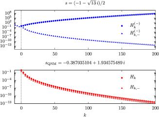
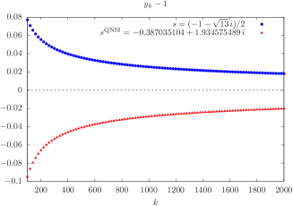
Figure 1: Top Panel: for $s^{(-)}_{0}=(-1-\sqrt{13}\,i)/2$ (top plot), $\{H^{(-)}_{k}\}$ grows as $k^{\zeta}e^{\kappa\sqrt{k}}$ for $k\gg 1$, while $\{H^{(-)}_{k,-}\}$ does not satisfy $H^{(-)}_{k,-}=0$ for $k<0$. For $s=s^{\rm QNM}$ (bottom plot) both sequences become linearly dependent. Bottom panel: For $s^{(-)}_{0}=(-1-\sqrt{13}\,i)/2$ (blue circle), $y_{k}-1>0$ contradicting the choice made in Eq. (44) of Ref. Batic et al. (2018). For $s=s^{\rm QNM}$ (red triangle) one obtains $y_{k}-1<0$ as expected.

Alternatively, we construct Ansorg and Panosso Macedo (2016); Panosso Macedo et al. (2018) a decaying solution $\{H^{(-)}_{k,-}\}$. We satisfy — by construction — the choice for the negative sign in Eq. (44) of Ref. Batic et al. (2018). The initial condition (12) is not satisfied because $H^{(-)}_{-1,-}\neq 0$ (blue triangles in the top panel of Fig. 1). If the decaying asymptotic properties required by condition (II) is satisfied, then condition (III) is not met.

Such results are explicit counterexamples to the key arguments of their proof. One identifies the same incompatibility between conditions (II) and (III) for other values of $n$ and $\ell$.

For the sake of comparison, the middle panel of Fig. 1 shows the equivalent results for the first well-known QNM with $\ell=2$: $s^{\rm QNM}=-0.3870351+1.93457545\,i$. The exponential decay for $\{H_{k}\}$ associated to the minimal solution of the recurrence relation is evident. It is also clear that $\{H_{k,-}\}$ satisfies the boundary condition (12) since $H_{-1,-}=0$. In other words, $\{H_{k}\}$ and $\{H_{k,-}\}$ become linearly dependent at the QNM, i.e., the same sequence satisfies conditions (II) and (III). The results for the QNMs are also displayed in the bottom panel of Fig. 1. Indeed, for a QNM, one has $y_{k}-1<0$.

New QNM branches. One can extend the arguments in Ref. Batic et al. (2018) to any value $s^{(\pm)}$ parametrised by (15). Following Ref. Batic et al. (2018), one starts with condition (II) and consider Eq. (16) in its generic form. One argues that “the case with the plus sign can be disregarded…” Batic et al. (2018) and we make a choice to work with the asymptotically decaying sequence $\{H^{(\pm)}_{k,-}\}_{k=0}^{\infty}$. Then, one considers the modified Gauss criterion for the generic $y_{k,-}$ exactly in the same way as in Ref. Batic et al. (2018). The convergence of $\sum_{k=0}^{\infty}H^{(\pm)}_{k,-}$ should be guaranteed when the inequality $2\rho\cos\phi>1$ is satisfied. Finally, one considers condition (III) and concludes: it is “straightforward to verify that we can recursively obtain all the unknown coefficients”, i.e, to obtain the sequence $\{H^{(\pm)}_{k}\}_{k=0}^{\infty}$. For example, the values $s^{(\pm)}(x)=x\left(-1\pm\sqrt{3}\,i\right)/2$ with $x\in{\mathbb{R}},$ $x>1$ meet all the requirements (including the inequality). They are clearly not another new branch of QNMs because the sequences satisfying conditions (II) and (III) are linearly independent.

Alternative methods. First, we consider the notion of resonances in scattering theory Dyatlov and Zworski (vres); Zworski (2017). We rewrite Eq. (Comment on “Some exact quasinormal frequencies of a massless scalar field in Schwarzschild spacetime”) as $-V_{,\tau\tau}+{\mathbf{L}}_{1}V_{,\tau}+{\mathbf{L}}_{2}V=0,$ with ${\mathbf{L}}_{1}$ (${\mathbf{L}}_{2}$) differential operators of first (second) order, acting only on $\sigma$. After a first order reduction in time, the QNMs are defined as the eigenvalues of the operator ${\mathbf{M}}=\left(\begin{array}[]{cc}0&{\mathbbm{1}}\\ {\mathbf{L}}_{2}&{\mathbf{L}}_{1}\end{array}\right).$ Figure 2 shows in red solid circles the eigenvalues of ${\mathbf{M}}$ for $\ell=2$ with the respective numerical errors. The values of the claimed new branch $s^{(-)}_{n}$ in Eq. (17) (empty blue circles) lie above the numerical error. They were not found in the spectrum of the operator ${\mathbf{M}}$.

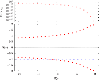
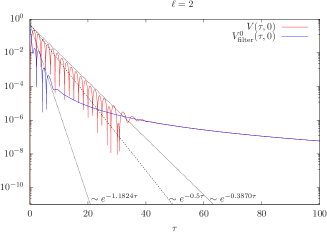
Figure 2: Top panel: QNMs as the spectra of the operator ${\mathbf{M}}$ (solid red circles). The extra panel display the numerical error to each QNM. The values $s^{(-)}_{n}$ in Eq. (17) (empty blue circles) are not found as eigenvalues of ${\mathbf{M}}$. Bottom: Time evolution (red) according to Panosso Macedo and Ansorg (2014). The filtered field (blue) shows the second QNM $s_{1}^{\rm QNM}$. No mode with $s_{0}^{\rm new}=(-1-\sqrt{13}i)/2$ is detected in the evolution.

Finally, we consider the direct time integration of Eq. (Comment on “Some exact quasinormal frequencies of a massless scalar field in Schwarzschild spacetime”) Panosso Macedo and Ansorg (2014). Though $V(\tau,\sigma)$ contains information about all the QNMs of the system, the one with slowest damping scale dominates. If (17) were a new branch of QNM, the first value would be $s_{0}^{(-)}=(-1-\sqrt{13}\,i)/2$. Since $|\Re(s_{0}^{\rm QNM})|<|\Re(s_{0}^{(-)})|<|\Re(s_{1}^{\rm QNM})|$, its contribution to $V(\tau,\sigma)$ would decay faster than the one from $s_{0}^{\rm QNM}$, but still slower than $s_{1}^{\rm QNM}$. One attempt to access $s_{0}^{(-)}$ is to filter the contribution from $s_{0}^{\rm QNM}$. Reference Ansorg and Panosso Macedo (2016) allows us to independently calculate the amplitude associated to a given $s^{\rm QNM}_{n}$ and filter its contribution from $V(\tau,\sigma)$. The contribution of $s_{0}^{(-)}$ within the original signal $V(\tau,\sigma)$ after the filtering is not found.

Conclusion. We addressed conditions (I)-(III) characterising QNMs in Ref. Batic et al. (2018). Using Propositions 2 and 1, respectively, one can always construct sequences $\{H^{(-)}_{k,-}\}_{k=0}^{\infty}$ and $\{H_{k}\}_{k=0}^{\infty}$ that meet conditions (II) and (III). The proof that such sequences are linearly dependent at the values $s^{(-)}_{n}$ in Eq. (17) is lacking in Ref. Batic et al. (2018). In particular, explicit counterexamples illustrate that $\{H^{(-)}_{k,-}\}_{k=0}^{\infty}$ and $\{H^{-}_{k}\}_{k=0}^{\infty}$ are not the same at the values $s^{(-)}_{n}$ in (17). Moreover, since condition (I) is valid for any $s$ with $\Re(s)<0$, there should exist further new QNMs if the arguments in Ref. Batic et al. (2018) were flawless. The frequencies of the new branch were not found in the direct time evolution of the original wave equation+boundary conditions, and the new values are not eigenvalues of the operator associated to the problem. Thus, the announced new frequencies should not be regarded as quasinormal modes.