Multiloop Euler-Heisenberg Lagrangians, Schwinger pair creation, and the QED N - photon amplitudes

Abstract:

An update is given on our long-term effort to perform a three-loop check on the Affleck-Alvarez-Manton/Lebedev-Ritus exponentiation conjecture for the imaginary part of the Euler-Heisenberg Lagrangian, using 1+1 dimensional QED as a toy model. After reviewing the history and significance of the conjecture, we present trigonometric integral representations for the single electron loop contributions to the three-loop Lagrangian, and develop a symmetry-based method for the calculation of their weak-field expansion coefficients.

Nuovo Cim.  ([) 3]⟨#1 #3⟩ Nuovo Cim.  ([) 3][#1 #3] Nuovo Cim.  (／$k$) Nuovo Cim. missing (missing) missing12 Nuovo Cim.  (ε) Nuovo Cim. missing (missing) missing~q Nuovo Cim.  (／$$) L

1 Euler-Heisenberg Lagrangian and photon amplitudes

In 1936 Heisenberg and Euler [1] calculated what nowadays is called the one-loop QED effective Lagrangian in a constant field (“ Euler-Heisenberg Lagrangian” = EHL), obtaining the following well-known integral representation:

$${\cal L}^{(1)}(a,b) = -{1\over 8\pi^{2}}\int_{0}^{\infty}{dT\over T^{3}}\,\,{\rm e}^{-m^{2}T}\biggl{[}{(eaT)(ebT)\over{\rm tanh}(eaT)\tan(ebT)}-{e^{2}\over 3}(a^{2}-b^{2})T^{2}-1\biggr{]}\,.$$

Here $a,b$ are the two invariants of the Maxwell field, related to $\bf E$, $\bf B$ by $a^{2}-b^{2}=B^{2}-E^{2},\quad ab={\bf E}\cdot{\bf B}$. The superscript $(1)$ stands for one-loop. A similar representation was obtained shortly later for scalar QED by Weisskopf [2].

The EHL holds the information on the $N$ - photon amplitudes in the low energy limit, where all photon energies are small compared to the electron mass, $\omega_{i}\ll m$ . Diagrammatically, this corresponds to Fig. 1

Figure 1: Sum of diagrams equivalent to the one-loop EHL

In [3] it was shown how to construct these amplitudes explicitly from the weak field expansion coefficients $c_{kl}$, defined by

$${\cal L}^{(1)}(a,b)=\sum_{k,l}c_{kl}\,a^{2k}b^{2l}\,.$$ (1)

In particularly, there it was shown that, for each $N$ and each given helicity assignment, the dependence on the momentum and polarization vectors can be absorbed into a single invariant $\chi_{N}$.

2 Imaginary part and Sauter-Schwinger pair creation

If the field has an electric component ($b\neq 0$) then there are poles on the integration contour at $ebT=k\pi$ which create an imaginary part. For the purely electric case one gets [4]

$${\rm Im}{\cal L}^{(1)}(E) = \frac{m^{4}}{8\pi^{3}}\beta^{2}\,\sum_{k=1}^{\infty}\frac{1}{k^{2}}\,\exp\left[-\frac{\pi k}{\beta}\right]$$ (2)

($\beta=eE/m^{2}$). Physically, in this decomposition the $k$th term relates to coherent creation of $k$ pairs in one Compton volume. In the following we will consider only the weak-field limit $\beta\ll 1$, where only the leading $k=1$ is relevant. Note that ${\rm Im}{\cal L}^{(1)}(E)$ depends on $E$ non-perturbatively (nonanalytically), which is consistent with the interpretation of pair creation as vacuum tunneling, originally due to Sauter, where a virtual electron-positron pair turns real by extracting their rest mass energies from the external field (Fig. 2).

Figure 2: Pair creation by an external field.

This connection between the effective action and the pair creation rate is based on the Optical Theorem, which relates the imaginary part of the diagrams shown in Fig. 1 to the “ cut diagrams ” shown in Fig. 3.

         

Figure 3: “Cut” diagrams describing Schwinger pair creation.

However, the latter individually all vanish for a constant field, which can emit only zero-energy photons. Thus for a constant field we cannot use dispersion relations for individual diagrams; what counts is rather the asymptotic behaviour of the diagrams for a large number of photons. The appropriate generalization is then a Borel dispersion relation. This works in the following way [5]: define the weak field expansion coefficients of the EHL by

$${\cal L}^{(1)}(E)=\sum_{n=2}^{\infty}c(n)\Bigl{(}\frac{eE}{m^{2}}\Bigr{)}^{2n}\,.$$ (3)

It can be shown that their leading large - $n$ behavior is

$$c(n)\,\,{\stackrel{{\scriptstyle n\to\infty}}{{\sim}}}\,\,c_{\infty}\Gamma[2n-2]\,.$$ (4)

The Borel dispersion relation relates this leading behavior to the leading weak-field behavior of the imaginary part of the Lagrangian:

$${\rm Im}{\cal L}^{(1)}(E)\,\,{\stackrel{{\scriptstyle\beta\to 0}}{{\sim}}}\,\,c_{\infty}\,\,{\rm e}^{-\frac{\pi m^{2}}{eE}}\,.$$ (5)

Thus we have rederived the leading Schwinger exponential of (2) in a way that might seem rather indirect and complicated. However, this approach turns out to be very useful for higher-loop considerations.

3 Beyond one loop

The two-loop (one-photon exchange) correction to the EHL corresponds to the set of diagrams shown in Fig. 4 (there is also a one-particle reducible contribution [6], but for our present purposes it can be discarded).

Figure 4: Feynman diagrams correposnding to the 2-loop EHL.

The corresponding corrections to the tree-level pair creation diagrams of Fig. 3 are shown in Fig. 5.

Figure 5: Feynman diagrams contributing to 2-loop Schwinger pair creation.

Even at the two-loop level, the study of the EHL has already a quite substantial history [7, 8, 9, 10]. Unfortunately, it leads to a type of rather intractable two-parameter integrals. However, the imaginary part ${\rm Im}{\cal L}^{(2)}(E)$ admits a decomposition similar to Schwinger’s one-loop one, eq. (2), and in the weak-field limit it becomes a simple addition to it [8]:

$${\rm Im}{\cal L}^{(1)}(E)+{\rm Im}{\cal L}^{(2)}(E)\,\,\,\,{\stackrel{{\scriptstyle\beta\to 0}}{{\sim}}}\,\,\,\,\frac{m^{4}\beta^{2}}{8\pi^{3}}\bigl{(}1+\alpha\pi\bigr{)}\,{\rm e}^{-{\pi\over\beta}}\,.$$

In [8], Lebedev and Ritus further noted that, if one assumed that higher orders will lead to exponentiation,

$${\rm Im}{\cal L}^{(1)}(E)+{\rm Im}{\cal L}^{(2)}(E)+{\rm Im}{\cal L}^{(3)}(E)+\ldots\,\,\,\,{\stackrel{{\scriptstyle\beta\to 0}}{{\sim}}}\,\,\,\,\frac{m^{4}\beta^{2}}{8\pi^{3}}\,{\rm exp}\Bigl{[}-{\pi\over\beta}+\alpha\pi\Bigr{]}={\rm Im}{\cal L}^{(1)}(E)\,\,{\rm e}^{\alpha\pi}$$

then the result could be interpreted in the tunneling picture as the corrections to the Schwinger pair creation rate due to the pair being created with a negative Coulomb interaction energy. This lowers the energy that has to be drawn from the field, and can be interpreted as a mass shift

$$m(E)\approx m+\delta m(E),\quad\delta m(E)=-\frac{\alpha}{2}\frac{eE}{m}$$

where $\delta m(E)$ is just the “Ritus mass shift”, originally derived from the crossed process of one-loop electron propagation in the field [11].

Unbeknownst to those authors, for scalar QED the corresponding exponentiation had been conjectured already two years earlier by Affleck, Alvarez and Manton [12]:

$$\sum_{l=1}^{\infty}{\rm Im}{\cal L}^{(l)}_{\rm scal}(E) {\stackrel{{\scriptstyle\beta\to 0}}{{\sim}}} -\frac{m^{4}\beta^{2}}{16\pi^{3}}\,{\rm exp}\Bigl{[}-{\pi\over\beta}+\alpha\pi\Bigr{]}={\rm Im}{\cal L}^{(1)}_{\rm scal}(E)\,\,{\rm e}^{\alpha\pi}\,.$$

However, they arrived at this conjecture in a very different way, namely using Feynman’s worldline path integral formalism in a semi-classical approximation ( “worldline instanton”).

Thus, although neither derivation is rigorous, there is much that speaks for the exponentiation conjecture. If true, it would constitute a unique example of a double summation of an infinite set of Feynman diagrams, involving any number of loops and legs, depicted in Fig. 6.

Figure 6: Feynman diagrams contributing to the AAM formula.

Here it is understood that the “horizontal” summation is performed using the leading large $n$ approximation for the weak-field expansion coefficients, which at each fixed loop order produces the same leading Schwinger exponential ${\rm e}^{-\frac{\pi}{\beta}}$. The “vertical” summation over an increasing number of internal photon insertions produces the Affleck-Alvarez-Manton/Lebedev-Ritus factor ${\rm e}^{\alpha\pi}$. Note that diagrams with more than one electron loop are nor included, since they get suppressed in the weak-field/large $n$ limit. On the other hand, the counterdiagrams from mass renormalization, although not shown here, have to be included. What is very surprising about the “vertical” exponentiation is, that it has produced the analytic factor ${\rm e}^{\alpha\pi}$! This is counter-intuitive, since the growth in the number of diagrams caused by the insertion of an increasing number of photons into an electron loop would lead one to expect a vanishing radius of convergence in $\alpha$.

Let us mention also that, using Borel analysis, this factor can be transferred from the imaginary part of the effective Lagrangian to the large - $N$ limit of the $N$ - photon amplitudes with all “+” polarizations [13]:

$${\rm lim}_{N\to\infty}{\Gamma^{({\rm all-loop})}[k_{1},\varepsilon_{1}^{+};\ldots;k_{N},\varepsilon_{N}^{+}]\over\Gamma^{(1)}[k_{1},\varepsilon_{1}^{+};\ldots;k_{N},\varepsilon_{N}^{+}]}=\,{\rm e}^{\alpha\pi}\,.$$

Here an essential ingredient is the above-mentioned fact that, independently of the loop order, the complete dependence of the $N$ - photon amplitudes for a fixed helicity assignment can be absorbed into a single invariant.

4 The EHL in 1+1 dimensional QED

The exponentiation conjecture has been verified at the two-loop order by explicit computation in both scalar and spinor QED. A three-loop check is in order, but calculating the three-loop EHL in $D=4$ seems presently technically out of reach. In 2005, Krasnansky [14] studied the EHL for scalar QED in various spacetime dimensions. In 1+1 dimensions, he found the following explicit result for this Lagrangian:

$${\cal L}_{\rm scal}^{(2)(2D)}(\kappa) = -\frac{e^{2}}{32\pi^{2}}\left(\xi^{2}_{2D}-4\kappa\xi_{2D}^{\prime}\right),$$

where $\xi_{2D}=-\Bigl{(}\psi(\kappa+{1\over 2})-\ln(\kappa)\Bigr{)}$, $\psi(x)=\Gamma^{\prime}(x)/\Gamma(x)$, $\kappa=m^{2}/(2ef)$, $f^{2}={1\over 4}F_{\mu\nu}F^{\mu\nu}$.

This is simpler than in four dimensions, but still non-trivial (in fact very similar in structure to the EHL in four dimensions for a self-dual field [16]), which suggests to use 1+1 dimensional QED as a toy model for testing the exponentiation conjecture. In [17] two of the authors and G. McKeon used the method of [12] to generalize the exponentiation conjecture to the 2D case, in the following form:

$${\rm Im}{\cal L}^{(all-loop)}_{2D}\sim\,{\rm e}^{-\frac{m^{2}\pi}{eE}+\tilde{\alpha}\pi^{2}\kappa^{2}}$$ (6)

where $\tilde{\alpha}=\frac{2e^{2}}{\pi m^{2}}$ is our definition of the fine-structure constant in 2D. There we also calculated the one- and two-loop contributions to the $2D$ EHL, obtaining (dropping now the subscript ‘2D’)

$${\cal L}^{(1)}(\kappa) = -{m^{2}\over 4\pi}{1\over\kappa}\Bigl{[}{\rm ln}\Gamma(\kappa)-\kappa(\ln\kappa-1)+{1\over 2}\ln\bigl{(}{\kappa\over 2\pi}\bigr{)}\Bigr{]}\,,$$

$${\cal L}^{(2)}(\kappa) = {m^{2}\over 4\pi}\frac{\tilde{\alpha}}{4}\Bigl{[}\tilde{\psi}(\kappa)+\kappa\tilde{\psi}^{\prime}(\kappa)+\ln(\lambda_{0}m^{2})+\gamma+2\Bigr{]}\,,$$

where $\tilde{\psi}(x)\equiv\psi(x)-\ln x+{1\over 2x}$. This allowed us to obtain explicit formulas not only for $c^{(1)}(n)$ but also for $c^{(2)}(n)$:

$$c^{(1)}(n) = (-1)^{n+1}\frac{B_{2n}}{4n(2n-1)}\,,$$

$$c^{(2)}(n) = (-1)^{n+1}\frac{\tilde{\alpha}}{8}\frac{2n-1}{2n}B_{2n}\,.$$

Using properties of the Bernoulli numbers $B_{n}$, it was then easy to verify the following prediction made by the exponentiation conjecture for the ratio between the two-loop and the one-loop expansion coefficients:

$$\lim_{n\to\infty}{c^{(2)}(n)\over c^{(1)}(n+1)} = \tilde{\alpha}\pi^{2}$$

(the relative shift in the argument of the coefficients is due to the fact that, unlike the four-dimensional case, in two dimensions the term involving $\tilde{\alpha}$ in the exponent in (6) also involves the external field). The convergence of $c^{(2)}(n)$ to the asymptotic prediction is rather fast (Fig. 7):

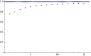
Figure 7: Convergence of the two-loop coefficients to the asymptotic prediction.

5 The three-loop EHL in 1 + 1 dimensional QED

At the three-loop level, the calculation of the EHL becomes challenging even in the two-dimensional case. There are five different topologies of diagrams, but for the exponentiation conjecture only the diagrams with a single electron loop are relevant, depicted in Fig. 8.

A                                 B

Figure 8: Single electron-loop contributions to the three-loop EHL.

We note that, due to the super-renormalizability of two-dimensional QED, at three loops the EHL is already UV finite. There are spurious IR - divergences, but we found that they can be removed by going to the “traceless” or “anti-Feynman” gauge $\xi=-1$. Although this gauge is known to have some special properties (see [15] and A. Kataev’s talk at this workshop) it is not clear to us why this is the case. Both diagrams lead to four-parameter integrals with a trigonometric integrand. The one for diagram A is simple:

$${\cal L}^{3A}(f) = \frac{\tilde{\alpha}^{2}m^{2}}{32\pi}\int_{0}^{\infty}dwdw^{\prime}d\hat{w}d\bar{w}~{}I_{A}~{}\,{\rm e}^{-a}\,,$$

$$I_{A} = \frac{\rho^{3}}{A^{2}\cosh\rho w\cosh\rho\hat{w}(\cosh\rho\bar{w}\cosh\rho w^{\prime})^{2}}\Bigg{[}\frac{\cosh\rho(w-\hat{w})}{2\rho}-\frac{1}{A\cosh\rho w\cosh\rho\hat{w}}\Bigg{]}\,,$$

where $\rho=\frac{ef}{m^{2}},a=w+w^{\prime}+\hat{w}+\bar{w},A=\rm tanh\rho w+\rm tanh\rho w^{\prime}+\rm tanh\rho\hat{w}+\rm tanh\rho\bar{w}$. The calculation of its contribution to the weak-field expansion coefficients $c^{(3)A}(n)=\frac{\tilde{\alpha}^{2}}{64}\Gamma^{A}_{n}$ is straightforward, and yields rational numbers. The first few are

$$\Gamma^{A}_{0}=-\frac{1}{3},\Gamma^{A}_{1}=-\frac{1}{30},\Gamma^{A}_{2}=\frac{17}{63},\Gamma^{A}_{3}=\frac{251}{99},\ldots$$ (7)

(so far we have obtained 13 coefficients). As one would expect, the nonplanar diagram B leads to a more complicated integrand:

$${\cal L}^{3B}(f) = \frac{\tilde{\alpha}^{2}m^{2}}{128\pi}\int_{0}^{\infty}dwdw^{\prime}d\hat{w}d\bar{w}~{}I_{B}~{}\,{\rm e}^{-a}\,,$$

$$I_{B} = \frac{\rho^{3}}{\cosh^{2}\rho w\cosh^{2}\rho w^{\prime}\cosh^{2}\rho\hat{w}\cosh^{2}\rho\bar{w}}\frac{B}{A^{3}C}$$

$$-\rho\frac{\cosh(\rho\tilde{w})}{\cosh\rho w\cosh\rho w^{\prime}\cosh\rho\hat{w}\cosh\rho\bar{w}}\Bigl{[}\frac{1}{A}-\frac{C}{G^{2}}\ln\Bigl{(}1+\frac{G^{2}}{AC}\Bigr{)}\Bigr{]}\,,$$

$$B = (\rm tanh^{2}z+\rm tanh^{2}\hat{z})(\rm tanhz^{\prime}+\rm tanh\bar{z})+(\rm tanh^{2}z^{\prime}+\rm tanh^{2}\bar{z})(\rm tanhz+\rm tanh\hat{z})\,,$$

$$C = \rm tanhz\,\rm tanhz^{\prime}\,\rm tanh\,\hat{z}+\rm tanhz\,\rm tanhz^{\prime}\,\rm tanh\bar{z}+\rm tanhz\,\rm tanh\hat{z}\,\rm tanh\bar{z}+\rm tanhz^{\prime}\,\rm tanh\hat{z}\,\rm tanh\bar{z}\,,$$

$$G = \rm tanhz\,\rm tanh\hat{z}-\rm tanhz^{\prime}\,\rm tanh\bar{z}$$

($z=\rho w$ etc.). For diagram $B$, the calculation of the weak-field expansion coefficients turned out to be much more difficult than for $A$. This is not only because the integrals are of a more difficult structure, and this time produce also $\zeta_{3}$ values, but also because the expansion in the external field creates huge numerator polynomials in the Feynman parameters. In a first attempt using numerical integration [18] we obtained only six coefficients, which is much too few for our purposes. In a forthcoming paper, we show how to use the high symmetry of diagram B to solve both problems. For obtaining a first integral, we introduce the operator

$$\tilde{d} \equiv \frac{\partial}{\partial w}-\frac{\partial}{\partial w^{\prime}}+\frac{\partial}{\partial\hat{w}}-\frac{\partial}{\partial\bar{w}}$$

which acts simply on the building blocks of the integrand. Integrating by parts with this operator, it is possible to write the integrand of the $n$-th coefficient $\beta_{n}$ as a total derivative $\beta_{n}=\tilde{d}\theta_{n}$. Then, using again the symmetries of diagram B,

$$\int_{0}^{\infty}dwdw^{\prime}d\hat{w}d\bar{w}\,\,{\rm e}^{-a}\beta_{n} = \int_{0}^{\infty}dwd\bar{w}d\hat{w}dw^{\prime}\tilde{d}\,\,{\rm e}^{-(w+w^{\prime}+\hat{w}+\bar{w})}\theta_{n}=4\int_{0}^{\infty}dwdw^{\prime}d\hat{w}\,\,{\rm e}^{-(w+w^{\prime}+\hat{w})}\,\theta_{n}|_{\bar{w}=0}\,.$$

The remaining integrals are already of a standard type. In this way we obtained the first two coefficients:

$$\Gamma^{B}_{0} = -\frac{3}{2}+\frac{7}{4}\zeta_{3},\quad\Gamma^{B}_{1}=-\frac{251}{120}+\frac{35}{16}\zeta_{3}\,.$$ (8)

We can also predict that all coefficients will be of the form $r_{1}+r_{2}\zeta_{3}$ with rational numbers $r_{1},r_{2}$.

For the purpose of obtaining more compact Feynman numerator polynomials, we note that Diagram $B$ has the symmetries

$$\qquad w \leftrightarrow \hat{w}$$

$$\quad w^{\prime} \leftrightarrow \bar{w}$$

$$\quad(w,\hat{w}) \leftrightarrow (w^{\prime},\bar{w})$$

Those generate the dihedral group $D_{4}$. Using the theory of polynomial invariants of that group, this allows one to rewrite the numerator polynomials as polynomials in the variable $\tilde{w}\equiv w-w^{\prime}+\hat{w}-\bar{w}$ with coefficients that are polynomials in the four $D_{4}$ - invariants $a,v,j,h$,

$$a = w+w^{\prime}+\hat{w}+\bar{w}\,,$$

$$v = 2(w\hat{w}+w^{\prime}\bar{w})+(w+\hat{w})(w^{\prime}+\bar{w})\,,$$

$$j = a\tilde{w}-4(w\hat{w}-w^{\prime}\bar{w})\,,$$

$$h = a(ww^{\prime}\hat{w}+ww^{\prime}\bar{w}+w\hat{w}\bar{w}+w^{\prime}\hat{w}\bar{w})+(w\hat{w}-w^{\prime}\bar{w})^{2}\,.$$

These invariants are moreover chosen such that they are annihiliated by $\tilde{d}$. Thus they are well-adapted to the integration-by-parts algorithm. This very significantly reduces the size of the expressions generated by the expansion in the field.

6 Outlook

To summarize, we are confident to get enough expansion coefficients to settle the question of the validity of the exponentiation conjecture in $1+1$ dimensional QED by the time of Loops and Legs 2020. The techniques that we have developed for the calculation of the 3-loop EHL in 2D should also become useful in an eventual calulation of this Lagrangian in four dimensions.

References

• [1] W. Heisenberg, H. Euler, Z. Phys. 98 (1936) 714.
• [2] V. Weisskopf, K. Dan. Vidensk. Selsk. Mat. Fy. Medd. 14 (1936) 1.
• [3] L. C. Martin, C. Schubert and V. M. Villanueva Sandoval, Nucl. Phys. B 668 (2003) 335, arXiv:hepth/0301022.
• [4] J. Schwinger, Phys. Rev. 82 (1951) 664.
• [5] G.V. Dunne and C. Schubert, Nucl. Phys. B 564 (2000) 59, hep-th/9907190.
• [6] H. Gies and F. Karbstein, JHEP 1703 (2017) 108, arXiv:1612.07251 [hep-th].
• [7] V. I. Ritus, Zh. Eksp. Teor. Fiz 69 (1975) 1517 [Sov. Phys. JETP 42 (1975) 774].
• [8] S. L. Lebedev, V. I. Ritus, Zh. Eksp. Teor. Fiz. 86 (1984) 408 [JETP 59 (1984) 237].
• [9] W. Dittrich and M. Reuter, Effective Lagrangians in Quantum Electrodynamics, Springer 1985.
• [10] M. Reuter, M. G. Schmidt and C. Schubert, Ann. Phys. (N.Y.) 259 313 (1997), hep-th/9610191.
• [11] V.I. Ritus, Zh. Eksp. Teor. Fiz. 75 (1978) 1560 [JETP 48 (1978) 788].
• [12] I.K. Affleck, O. Alvarez and N.S. Manton, Nucl. Phys. B 197 (1982) 509.
• [13] G.V. Dunne and C. Schubert, J. Phys.: Conf. Ser. 37 (2006) 59, hep-th/0409021.
• [14] M. Krasnansky, Int. J. Mod. Phys. A 23, 5201 (2008), hep-th/0607230.
• [15] A. V. Garkusha, A. L. Kataev and V. S. Molokoedov, JHEP 1802 (2018) 161, arXiv:1801.06231 [hep-ph].
• [16] G. V. Dunne and C. Schubert, JHEP 0208, 053 (2002), hep-th/0205004.
• [17] I. Huet, D.G.C. McKeon and C. Schubert, JHEP 1012 036 (2010), arXiv:1010.5315 [hep-th].
• [18] I. Huet, M. Rausch de Traubenberg and C. Schubert, Adv. High Energy Phys. 2017 (2017) 6214341, arXiv:1707.07655 [hep-th].