DCPT-18/21

The twistor Wilson loop and the amplituhedron

Paul Heslop and Alastair Stewart

Mathematics Department, Durham University, Science Laboratories,
South Rd, Durham DH1 3LE

Abstract

The amplituhedron provides a beautiful description of perturbative superamplitude integrands in ${\mathcal{N}}=4$ SYM in terms of purely geometric objects, generalisations of polytopes. On the other hand the Wilson loop in supertwistor space also gives an explicit description of these superamplitudes as a sum of planar Feynman diagrams. Each Feynman diagram can be naturally associated with a geometrical object in the same space as the amplituhedron (although not uniquely). This suggests that these geometric images of the Feynman diagrams give a tessellation of the amplituhedron. This turns out to be the case for NMHV amplitudes. We prove however that beyond NMHV this is not true. Specifically, each Feynman diagram leads to an image with a physical boundary and spurious boundaries. The spurious ones should be “internal”, matching with neighbouring diagrams. We however show that there is no choice of geometric image of the Wilson loop Feynman diagrams which yields a geometric object without leaving unmatched spurious boundaries.

1 Introduction

Scattering amplitudes in planar ${\mathcal{N}}=4$ SYM have long been a fruitful source of new concepts and techniques in quantum field theory. One of the most exciting recent discoveries relates their perturbative integrands directly to geometric objects. This was first noticed by Hodges [1], and was further developed by Arkani-Hamed et al [2]. Arkani-Hamed and Trnka then interpreted the integrands as being equivalent to generalised polyhedra in positive Grassmannians called ‘amplituhedra’ [3]. This has lead to a great deal of interest from both physicists and mathematicians as well as a number of generalisations [4, 5, 6, 7, 8, 9, 10, 11, 12, 13, 14, 15, 16, 17, 18, 19, 20, 21, 22, 23, 24, 25, 26, 27, 28, 29].

Although early polytope interpretations [1, 2] involved considering amplitudes via twistor Wilson loop diagrams (WLDs) the amplituhedron itself instead arose from considering the BCFW method of obtaining amplitudes. However the WLDs apparently lend themselves very naturally and directly to a geometrical interpretation and in this paper we wish to look again at the relationship between WLDs and the amplituhedron. Previous work also examining this connection includes [9, 18, 26]. In particular in [26] it was shown that the WLDs give a very natural description of the physical boundary of the amplituhedron. Specifically here we wish to examine whether it is possible to use WLDs to define a tessellation of the amplituhedron or more generally a tessellation of any “good” geometrical shape, whereby “good” means it only has a physical boundary (corresponding to poles of the amplitude) without any spurious boundaries. We prove that beyond NMHV this is not the case. The WLDs do not give a tessellation of the amplituhedron or any other geometrical object without remaining unmatched spurious boundaries.

Let us emphasise that we make no assumptions about positivity, or convexity or any particular specific form for this geometrical shape. Our only assumptions are that each WLD is associated with a region of amplituhedron space in such a way that the canonical form [30] of that region gives back the WLD. Since each WLD contains spurious poles which have a geometrical interpretation as spurious boundaries we then ask if it is possible to choose these regions in such a way that all spurious boundaries glue together correctly pairwise with those of other diagrams so that the union of regions leaves no remaining unmatched spurious boundaries. This turns out to be impossible.

Many of the salient points can be illustrated in the toy model for the amplituhedron introduced in [3] consisting simply of polygons in $P^{2}$ with $n$ vertices $Z_{i}\in P^{2}$. The map from this polygon $X$ to the algebraic “amplitude” $\Omega(X)$ is made by associating a “canonical form” with the geometry. This canonical form is a differential volume form with logarithmic divergences on the boundary of the polygon and no divergences inside it. Such differential forms are not easy to obtain directly [30], but have the helpful feature that the volume form of the union of (non-overlapping) polygons gives the sum of the volume forms for each i.e. $\Omega(X_{1}\cup X_{2})=\Omega(X_{1})+\Omega(X_{2})$. This gives a simple means of obtaining the canonical form for a polygon by triangulating it and summing the canonical forms for each triangle.

A simple way to obtain the canonical form for a triangle with vertices $Z_{1},Z_{2},Z_{3}$ is to choose coordinates $a,b$ such that the inside of the triangle coincides with the region $a,b>0$ i.e. $Y=aZ_{1}+bZ_{2}+Z_{3}$. Then the canonical form is simply $\mathop{}\!\mathrm{d}a\mathop{}\!\mathrm{d}b/(ab)$ which can then be rewritten in a co-ordinate independent way as $\langle Y\mathop{}\!\mathrm{d}^{2}Y\rangle\langle 123\rangle^{2}/(\langle Y12\rangle\langle Y23\rangle\langle Y31\rangle)$. Two adjacent triangles with vertices $Z_{1},Z_{2},Z_{3}$ and $Z_{1},Z_{3},Z_{4}$ triangulate a quadrilateral with vertices $Z_{1},Z_{2},Z_{3},Z_{4}$. Each individual triangle has a boundary $[Z_{1}Z_{3}]$ which is not a boundary of the quadrilateral. Such a boundary is referred to as “spurious”. Similarly each canonical form has a corresponding log divergence when $Y$ approaches this boundary, $Y\rightarrow\alpha Z_{1}+\beta Z_{3}$. However in the sum of the two canonical forms, $\langle 123\rangle^{2}/(\langle Y12\rangle\langle Y23\rangle\langle Y31\rangle)+\langle 134\rangle^{2}/(\langle Y13\rangle\langle Y34\rangle\langle Y41\rangle)$ the residues of the two poles cancel there and the resulting canonical form indeed only has log divergences on the boundary of the quadrilateral itself.

Although there is a unique canonical form associated to a polygon, the reverse is not true. For example, given the canonical form for the triangle with vertices $Z_{1},Z_{2},Z_{3}$, $\langle Y\mathop{}\!\mathrm{d}^{2}Y\rangle\langle 123\rangle^{2}/(\langle Y12\rangle\langle Y23\rangle\langle Y31\rangle)$, there are four inequivalent triangles in $P^{2}$ with this canonical form. These are given by the set $\{Y:Y=aZ_{1}+bZ_{2}+Z_{3}\}$ for the four choices $(a,b>0)$, $(a>0,b<0)$, $(a<0,b>0)$ or $(a<0,b<0)$. These are simply the four inequivalent triangles in $P^{2}$ with vertices $Z_{1},Z_{2},Z_{3}$ (see Figure 1a).

Figure 1: Figures illustrating polygons in $P^{2}$ represented as a disc where opposite points of the disc are identified. In Figure a) we illustrate the fact that there are four triangles $\mathrm{I,II,III,IV}$ all of which have the same three vertices $Z_{1},Z_{2},Z_{3}$ and all having the same canonical form $\langle 123\rangle^{2}/(\langle Y12\rangle\langle Y23\rangle\langle Y31\rangle)$. In Figure b) we see a region (shaded area) which has the same canonical form as the quadrilateral $[Z_{1}Z_{2}Z_{3}Z_{4}]$, $\langle 123\rangle^{2}/(\langle Y12\rangle\langle Y23\rangle\langle Y31\rangle)+\langle 134\rangle^{2}/(\langle Y13\rangle\langle Y34\rangle\langle Y41\rangle)$ but which does not represent a good geometrical region as it has spurious boundaries.

So the geometry associated with a given canonical form is not unique but only defined up to sign choices. If on the other hand we are given a canonical form, written as a sum of terms each containing spurious poles that cancel in the sum (which as we will see is precisely what WLDs give us), then the assigning of a geometrical region to each term (i.e. the choice of signs) can not be done independently for each term: the cancelling of spurious poles should correspond geometrically to a matching of the corresponding spurious boundaries (in Figure 1b we see a simple example of a region with the same canonical form as the quadrilateral $[Z_{1}Z_{2}Z_{3}Z_{4}]$ but with left over spurious boundaries).

There are two natural ways to triangulate a polygon illustrated in Figure 2. BCFW recursion for tree-level NMHV diagrams gives the natural (higher dimensional) analogue of the first way, triangulating to one of the vertices.

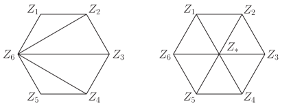
Figure 2: Two possibilities for triangulating a polygon. BCFW give a generalisation of the first whereas WLDs give a generalisation of the second (for NMHV).

Remarkably WLDs for the planar N^kMHV amplitude/ Wilson loop split the amplitude into well-defined pieces, each of which naturally yields a volume form on the space on which the amplituhedron lies, the Grassmannian $\text{Gr}(k,4{+}k)$. Each volume form has physical poles and spurious poles the latter of which all cancel in the sum over diagrams. The physical poles of the WLDs correspond to the physical boundary of the amplituhedron [26]. This therefore strongly suggests that the WLDs should correspond to be a tessellation of the amplituhedron. The canonical forms of each tile corresponding to WLDs. Note that if this were the case the WLDs would then give a very explicit tessellation of the amplituhedron.

In the NMHV tree-level case this intuition indeed turns out to be correct: each WLD can be straightforwardly associated with a tile in the tessellation of the amplituhedron. Indeed NMHV Twistor Wilson loop Feynman diagrams (WLDs) naturally give a higher dimensional analogue of the second way of tessellating polygons, introducing an additional vertex $Z_{*}$ and triangulating to that, Figure 2b.

In this paper we however prove that, for higher NMHV degree this is not the case. More concretely we prove that there do not exist a set of tiles whose canonical forms correspond to WLDs and which glue together to form a geometry without spurious boundaries. The WLDs can therefore not be associated with a tessellation of the amplituhedron or indeed any geometry whose boundary corresponds to only the physical poles of the amplitude.

Note added: The paper [31] by Susama Agarwala and Cameron Marcott dealing with the same problem as this paper was posted on the same day.

2 WLDs and volume forms

2.1 WLDs

Here, we provide a brief description of planar Wilson loops in ${\mathcal{N}}=4$ Super Yang Mills in super twistor space and define the WLDs that arise. We do not derive these here, for their derivation see [32, 33, 34].

The WLDs we are discussing here are simply the Feynman diagrams describing a polygonal holomorphic Wilson-loop in super twistor space with vertices being the super twistors $\mathcal{Z}_{1}\dots\mathcal{Z}_{n}\in{\mathbb{C}}^{4|4}$. In the planar theory this is equivalent, via the Wilson loop / amplitude duality [35, 36, 37], to $n$-point superamplitudes. At tree level the Feynman diagrams consist simply of propagators whose two ends lie on the Wilson loop contour. In the planar theory diagrams are only valid if we can draw all the propagators inside the Wilson loop without crossing. The N^kMHV Wilson loop is the sum over all such diagrams involving $k$ propagators (see Figure 3 for an example of a diagram contributing to 8-point N⁴MHV).

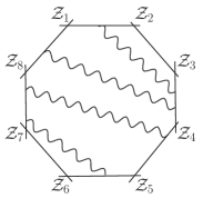
Figure 3: Example of a Wilson loop diagram which contributes to the $8$-point N⁴MHV amplitude.

To each propagator from edge $[{\mathcal{Z}}_{i}{\mathcal{Z}}_{i+1}]$ to $[{\mathcal{Z}}_{j}{\mathcal{Z}}_{j+1}]$ we assign the $(4|4)$ delta function:

(1)

We then integrate over the complex integration variables associated with each end of the propagator with a measure determined by all the propagators ending on the same edge

(2)

In Figure 4 we illustrate these rules with two examples firstly an example diagram contributing to the NMHV six-point amplitude and secondly one contributing to the N²MHV six-point amplitude.

$\begin{array}[]{m{8cm}m{8cm}}\includegraphics[scale={0.5}]{NMHVExample}&\includegraphics[scale={0.5}]{N2MHVExample}\\ $\int\frac{\mathop{}\!\mathrm{d}a\mathop{}\!\mathrm{d}b\mathop{}\!\mathrm{d}c\mathop{}\!\mathrm{d}d}{abcd}{\delta}^{4|4}\left(a{\mathcal{Z}}_{1}{+}b{\mathcal{Z}}_{2}{+}c{\mathcal{Z}}_{4}{+}d{\mathcal{Z}}_{5}{+}{\mathcal{Z}}_{*}\right)$&$\begin{array}[]{l}\int\frac{\mathop{}\!\mathrm{d}a_{1}\mathop{}\!\mathrm{d}b_{1}\mathop{}\!\mathrm{d}c_{1}\mathop{}\!\mathrm{d}d_{1}\mathop{}\!\mathrm{d}f_{1}\mathop{}\!\mathrm{d}g_{1}\mathop{}\!\mathrm{d}h_{1}}{a_{1}b_{1}g_{1}h_{1}e_{1}(c_{1}f_{1}-d_{1}e_{1})d_{1}}\times\\ \times\delta^{(4|4)}\left(a_{1}{\mathcal{Z}}_{1}{+}b_{1}{\mathcal{Z}}_{2}{+}c_{1}{\mathcal{Z}}_{3}{+}d_{1}{\mathcal{Z}}_{4}{+}{\mathcal{Z}}_{*}\right)\\ \times\delta^{(4|4)}\left(e_{1}{\mathcal{Z}}_{3}{+}f_{1}{\mathcal{Z}}_{4}{+}g_{1}{\mathcal{Z}}_{5}{+}h_{1}{\mathcal{Z}}_{6}{+}{\mathcal{Z}}_{*}\right)\end{array}$\end{array}$

Figure 4: Examples of Feynman diagrams in twistor space that contribute to the $6$-point NMHV / N²MHV amplitude with their corresponding expressions following the rules given.

2.2 Amplituhedron volume forms from WLDs

The WLDs are originally defined in supertwistor space, ${\mathbb{C}}^{4|4}$, but have a very direct interpretation as volume forms in the Grassmannian of $k$-planes in ${\mathbb{C}}^{4+k}$, $\text{Gr}(k,4{+}k)$ or “amplituhedron space”.

Essentially the integration variables and delta functions of the WLDs define coordinates in amplituhedron space, and the measure gives the volume form written in terms of these coordinates. All N^kMHV WLDs have the general form, following from the description in the previous subsection

$$\int\Omega_{4k}(a_{i})\delta^{k\times(4|4)}(C(a_{i}).{\mathcal{Z}})\qquad\text{[WLD]}$$ (3)

where $a_{i}$ are the $4k$ coordinates (4 for each of the $k$ propagators), $\Omega_{4k}(a_{i})$ is the integration measure (a $4k$-form obtained as a product of terms of the form (2)) and $\delta^{4k|4k}(C(a_{i}).{\mathcal{Z}})$ are the $k$ delta functions, one for each propagator as in (1), written as a $k\times(n{+}1)$ matrix $C(a_{i})$ acting on the external supertwistors ${\mathcal{Z}}$, themselves viewed as an $(n{+}1)\times(4|4)$ matrix. The corresponding volume form in $\text{Gr}(k,k{+}4)$ is then simply the measure $\Omega_{4k}(a_{i})$ where the coordinates are now reinterpreted as co-ordinates in $\text{Gr}(k,k{+}4)$ via the map

$$\Omega(Y)=\Omega_{4k}(a_{i})\qquad Y=C(a_{i}).Z\in\text{Gr}(k,k+4)$$ (4)

and $Z$ is here an $(n{+}1)\times(4+k)$ matrix, the external ${\mathcal{Z}}$s converted to $4+k$ dimensional bosonised supertwistors in the standard way described in [3].

We illustrate this using the two examples of Figure 4. For the NMHV example diagram of Figure 4a we read off the volume form:

$$\begin{array}[]{cl}\int\frac{\mathop{}\!\mathrm{d}a\mathop{}\!\mathrm{d}b\mathop{}\!\mathrm{d}c\mathop{}\!\mathrm{d}d}{abcd}\,{\delta}^{4|4}\left(a{\mathcal{Z}}_{1}{+}b{\mathcal{Z}}_{2}{+}c{\mathcal{Z}}_{4}{+}d{\mathcal{Z}}_{5}{+}{\mathcal{Z}}_{*}\right)&[\text{WLD}]\\ \downarrow\\ \Omega=\frac{\mathop{}\!\mathrm{d}a\mathop{}\!\mathrm{d}b\mathop{}\!\mathrm{d}c\mathop{}\!\mathrm{d}d}{abcd}\qquad Y=aZ_{1}{+}bZ_{2}{+}cZ_{4}{+}dZ_{5}{+}Z_{*}\in{\mathbb{C}}^{5}&\text{[Amplituhedron Volume form]}\end{array}$$ (8)

This volume form can be covariantised to be written in a coordinate independent way as

$$\frac{\langle Y\mathop{}\!\mathrm{d}^{4}Y\rangle\langle Z_{1}Z_{2}Z_{4}Z_{5}Z_{*}\rangle^{4}}{\langle YZ_{1}Z_{2}Z_{4}Z_{5}\rangle\langle YZ_{2}Z_{4}Z_{5}Z_{*}\rangle\langle YZ_{4}Z_{5}Z_{*}Z_{1}\rangle\langle YZ_{5}Z_{*}Z_{1}Z_{2}\rangle\langle YZ_{*}Z_{1}Z_{2}Z_{4}\rangle}\ ,$$ (9)

where the angle brackets denote $5\times 5$ determinants.

For the second N²MHV example diagram of Figure 4b we get

$$\begin{array}[]{cl}\int\frac{\mathop{}\!\mathrm{d}a_{1}\mathop{}\!\mathrm{d}b_{1}\mathop{}\!\mathrm{d}c_{1}\mathop{}\!\mathrm{d}d_{1}\mathop{}\!\mathrm{d}f_{1}\mathop{}\!\mathrm{d}g_{1}\mathop{}\!\mathrm{d}h_{1}}{a_{1}b_{1}g_{1}h_{1}e_{1}(c_{1}f_{1}-d_{1}e_{1})d_{1}}\delta^{(8|8)}\left(C_{1}\cdot\mathcal{Z}\right)&[\text{WLD}]\\ \downarrow\\ \Omega=\frac{\mathop{}\!\mathrm{d}a_{1}\mathop{}\!\mathrm{d}b_{1}\mathop{}\!\mathrm{d}c_{1}\mathop{}\!\mathrm{d}d_{1}\mathop{}\!\mathrm{d}f_{1}\mathop{}\!\mathrm{d}g_{1}\mathop{}\!\mathrm{d}h_{1}}{a_{1}b_{1}g_{1}h_{1}e_{1}(c_{1}f_{1}-d_{1}e_{1})d_{1}}\qquad Y=C_{1}.Z\in\text{Gr}(2,6)&\text{[Amplituhedron Volume form]}\end{array}$$ (13)

where ${\mathcal{Z}}=({\mathcal{Z}}_{1},{\mathcal{Z}}_{2},\dots\mathcal{Z}_{6},{\mathcal{Z}}_{*})^{T}$ are the external supertwistors (together with ${\mathcal{Z}}_{*}$) viewed as a $7\times(4|4)$ matrix,

$$C_{1}=\begin{pmatrix}a_{1}&b_{1}&c_{1}&d_{1}&0&0&1\\ 0&0&e_{1}&f_{1}&g_{1}&h_{1}&1\end{pmatrix}\in\text{Gr}(2,7)$$ (14)

and similarly $Z=(Z_{1},\dots Z_{6},Z_{*})^{T}$ are the external bosonised supertwistors (with $Z_{*}$) viewed as a $7\times 6$ matrix.

3 NMHV amplituhedron from WLDs

Let us first consider the NMHV case. Here the WLDs do give a good tessellation of the amplituhedron. Indeed WLDs were involved in the original polytope interpretation of amplitudes [1, 2].

The twistor Wilson loop description of the $n$-point NMHV amplitude is simply a sum over all diagrams consisting of a single propagator attached to any two edges of the polygon. Written as a volume form in $\text{Gr}(1,5)$ (amplituhedron space) the WLD corresponding to a propagator from edge $[Z_{i}Z_{i+1}]$ to edge $[Z_{j}Z_{j+1}]$ is (see (8))

$$\Omega=\frac{\mathop{}\!\mathrm{d}a\mathop{}\!\mathrm{d}b\mathop{}\!\mathrm{d}c\mathop{}\!\mathrm{d}d}{abcd}\qquad Y=aZ_{i}{+}bZ_{i+1}{+}cZ_{j}{+}dZ_{j+1}{+}Z_{*}\in{\mathbb{C}}^{5}$$ (15)

which written in a coordinate independent form is (9)

$$\frac{\langle Y\mathop{}\!\mathrm{d}^{4}Y\rangle\langle Z_{i}Z_{i+1}Z_{j}Z_{j+1}Z_{*}\rangle^{4}}{\langle YZ_{i}Z_{i+1}Z_{j}Z_{j+1}\rangle\langle YZ_{i+1}Z_{j}Z_{j+1}Z_{*}\rangle\langle YZ_{j}Z_{j+1}Z_{*}Z_{i}\rangle\langle YZ_{j+1}Z_{*}Z_{i}Z_{i+1}\rangle\langle YZ_{*}Z_{i}Z_{i+1}Z_{j}\rangle}\ .$$ (16)

So the full NMHV amplitude is thus

$$\Omega={\langle Y\mathop{}\!\mathrm{d}^{4}Y\rangle}$$

$$\times \sum_{i,j}\frac{\langle Z_{i}Z_{i+1}Z_{j}Z_{j+1}Z_{*}\rangle^{4}}{\langle YZ_{i}Z_{i+1}Z_{j}Z_{j+1}\rangle\langle YZ_{i+1}Z_{j}Z_{j+1}Z_{*}\rangle\langle YZ_{j}Z_{j+1}Z_{*}Z_{i}\rangle\langle YZ_{j+1}Z_{*}Z_{i}Z_{i+1}\rangle\langle YZ_{*}Z_{i}Z_{i+1}Z_{j}\rangle}\ .$$ (17)

It is clear from (15) that the spurious poles for each WLD arise when any one of $a,b,c,d\rightarrow 0$. In terms of the WLD we view this as one end of the propagator approaching a vertex. Then this spurious pole cancels with the spurious pole of a neighbouring diagram where the end of the propagator approaches the same vertex from the other side see Figure 5.

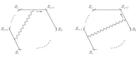
Figure 5: Spurious poles occur when the propagator end reaches the vertex. It is cancelled by the adjacent diagram. Imposing that this cancellation has a corresponding geometric meaning as a matching of spurious boundaries imposes a correlation between the sign choices for the geometric image of the two diagrams.

There is then a natural geometrical interpretation of (17) as a union of tiles, each giving one of the above terms as its canonical form. This is

$$\bigcup_{i,j}\{Y=aZ_{i}{+}bZ_{i{+}1}{+}cZ_{j}{+}dZ_{j{+}1}{+}Z_{*}\,;\,a,b,c,d\geq 0\}\subset{\text{Gr}}(1,5)\ .$$ (18)

Note here that we are using the same variables $(a,b,c,d)$ as given to us by the WLDs to describe the geometric region in question. However, whereas for the WLDs the integration is over complex space, here the variables are restricted to a subspace of the real line.

If the $Z_{i}$ are convex ($\langle Z_{i}Z_{j}Z_{k}Z_{l}Z_{m}\rangle>0$ for all cyclically ordered $Z_{i},Z_{j},Z_{k},Z_{l},Z_{m}$) this provides a tessellation of the amplituhedron as defined in [3]. Indeed this is analogous to the tessellation of the polygon in the toy model depicted in Figure 2b. But note that this defines a good geometrical region (i.e. one without spurious boundaries) even for non convex choices of external $Z_{i}$.

At this point it is interesting to ask how unique this region is. Are there any other ways of defining tiles whose canonical forms give the WLDs, and which would glue together to yield a geometry without spurious boundaries?

As illustrated for the toy model in Figure 1, any choice of signs for the variables $a,b,c,d$ in each tile would give a canonical form of the corresponding WLD. However if we choose arbitrary sign choices for each diagram differently, the spurious boundaries will not glue together properly, even though the spurious poles of the corresponding canonical forms would cancel (recall Figure 1b for an illustration of this sort of phenomenon for the toy model). Let us then consider a particular tile corresponding to the WLD with a propagator from edge $[Z_{i}Z_{i+1}]$ to edge $[Z_{j}Z_{j+1}]$. The most general geometry giving this canonical form (15,16) is

$$\{Y=as_{i}Z_{i}{+}bs_{i+1}Z_{i{+}1}{+}cs_{j}Z_{j}{+}ds_{j+1}Z_{j{+}1}{+}Z_{*}\,:\,a,b,c,d\geq 0\}$$ (19)

where $s_{i},s_{i+1},s_{j},s_{j+1}=\pm 1$ are four arbitrary sign choices. The spurious poles are here seen as spurious boundaries arising when any one of the four coordinates $a,b,c,d\rightarrow 0$ (whereas a fifth, physical boundary occurs when they all simultaneously $a,b,c,d\rightarrow\infty$). Let us focus on the spurious boundary when $a\rightarrow 0$. This must match the boundary when $b\rightarrow 0$ of the adjacent diagram with propagator from edge $[Z_{i+1}Z_{i+2}]$ to edge $[Z_{j}Z_{j+1}]$ (which we also define with arbitrary signs $s^{\prime}_{i+1},s^{\prime}_{i+2},s^{\prime}_{j},s^{\prime}_{j+1}=\pm 1$):

$$\begin{array}[]{c}\{Y=as_{i}Z_{i}{+}bs_{i+1}Z_{i{+}1}{+}cs_{j}Z_{j}{+}ds_{j+1}Z_{j{+}1}{+}Z_{*}\,:\,a=0,b,c,d\geq 0\}\\ =\\ \{Y=as^{\prime}_{i+1}Z_{i+1}{+}bs^{\prime}_{i+2}Z_{i{+}2}{+}cs^{\prime}_{j}Z_{j}{+}ds^{\prime}_{j+1}Z_{j{+}1}{+}Z_{*}\,:\,b=0,\ a,c,d\geq 0\}\end{array}$$ (23)

This mimics the corresponding discussion of cancellation of spurious poles in Figure 5 and associated discussion. Except now the geometrical matching imposes consistency conditions on the sign choices of the two tiles. For these spurious boundaries to match we clearly require

$$s_{i+1}=s^{\prime}_{i+1},\quad s_{j}=s^{\prime}_{j},\quad s_{j+1}=s^{\prime}_{j+1}.$$ (24)

Thus the signs associated with each vertex for different diagrams must be the same. Clearly a similar mechanism applies for matching boundaries when $c$ or $d\rightarrow 0$.

From this discussion one can see then that the most general geometry without spurious boundaries is obtained by assigning a fixed sign, $s_{i}=\pm 1$, to each vertex $Z_{i}$. So the region

$$\bigcup_{i,j}\{Y=as_{i}Z_{i}{+}bs_{i+1}Z_{i{+}1}{+}cs_{j}Z_{j}{+}ds_{j+1}Z_{j{+}1}{+}Z_{*}\,;\,a,b,c,d\geq 0\}\subset{\text{Gr}}(1,5)\$$ (25)

is the most general geometry matching the WLDs and without spurious boundaries. This is true for any choice of signs $s_{i}$. This is equivalent to simply considering the original amplituhedron with all positive signs but flipping the sign of the external $Z$’s. At most one choice of signs for the $Z$s can correspond to a convex shape.

For completeness we should also consider a special case of the spurious poles / boundaries cancellation which occurs when the propagator lies between next-to-adjacent edges, i.e. between edge $[Z_{i}Z_{i+1}]$ and edge $[Z_{i+2}Z_{i+3}]$. The spurious boundary when $a=0$ of this diagram at first sight looks like it is not present (propagators between adjacent edges are not allowed; they give vanishing results). Instead it matches with $d=0$ of the diagram with propagator between edge $[Z_{i+1}Z_{i+2}]$ and edge $[Z_{i+3}Z_{i+4}]$

$$\begin{array}[]{c}\{Y=as_{i}Z_{i}{+}bs_{i+1}Z_{i{+}1}{+}cs_{i+2}Z_{i+2}{+}ds_{i+3}Z_{i+3}{+}Z_{*}\,;\,a=0,b,c,d\geq 0\}\\ =\\ \{Y=as_{i+1}Z_{i+1}{+}bs_{i+2}Z_{i{+}2}{+}cs_{i+3}Z_{i+3}{+}ds_{i+4}Z_{i+4}{+}Z_{*}\,;\,d=0,\ a,b,c\geq 0\}\ .\end{array}$$ (29)

We see that the spurious boundaries indeed match for this special case too even for the general choice of signs.

4 $N^{2}$MHV

Having considered NMHV WLDs and shown how to obtain a “good” geometry from them (in many inequivalent ways) we now consider the same problem for higher MHV degree. We will prove that beyond NMHV the WLDs cannot in fact be glued together to form a geometry without spurious boundaries. To prove this, it is enough to show that there is no set of sign choices for the coordinates that is consistent with the matching of spurious boundaries. In order to illustrate the argument we focus on the case of $n=6$ below, however the argument applies to all $n$.

4.1 Cancellation of spurious poles in $N^{2}$MHV WLDs

Before considering the geometric image as spurious boundaries we consider the algebraic cancellation of spurious poles for N²MHV diagrams. The discussion of spurious poles considered in the previous section, arising when the ends of propagators approach vertices (see Figure 5) goes through in the same way for any MHV degree. However beyond NMHV a new type of spurious pole occurs in the integrals of WLDs. Since now we have two or more propagators, there exists the possibility that the ends of two different propagators can meet each other on an edge. This produces a pole in the WLD. There is an interesting three-way cancellation of this type of spurious pole between three related diagrams (see [38, 34] for previous work also describing this mechanism). An example set of diagrams is shown in Figure 6.

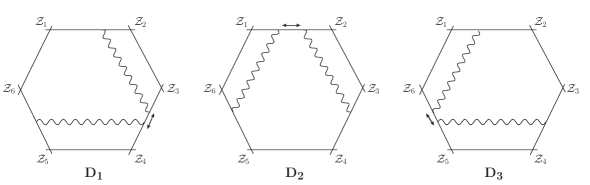
Figure 6: Three diagrams each having a new type of spurious pole occurring when the propagator ends touch. In the sum of the three diagrams however this pole cancels. Note that although this is drawn at six points for definiteness the cancellation only depends on the three sides taking part and can be directly repeated at $n$ points.

Using the rules from section 2.1, the integrals associated with the diagrams under consideration are

$$\mathcal{I}(D_{1})=\int\frac{\mathop{}\!\mathrm{d}a_{1}\mathop{}\!\mathrm{d}b_{1}\mathop{}\!\mathrm{d}c_{1}\mathop{}\!\mathrm{d}d_{1}\mathop{}\!\mathrm{d}e_{1}\mathop{}\!\mathrm{d}f_{1}\mathop{}\!\mathrm{d}g_{1}\mathop{}\!\mathrm{d}h_{1}}{a_{1}b_{1}g_{1}h_{1}e_{1}(c_{1}f_{1}-d_{1}e_{1})d_{1}}\delta^{(8|8)}\left(C_{1}\cdot\mathcal{Z}\right)$$ (30)

$$\mathcal{I}(D_{2})=\int\frac{\mathop{}\!\mathrm{d}a_{2}\mathop{}\!\mathrm{d}b_{2}\mathop{}\!\mathrm{d}c_{2}\mathop{}\!\mathrm{d}d_{2}\mathop{}\!\mathrm{d}e_{2}\mathop{}\!\mathrm{d}f_{2}\mathop{}\!\mathrm{d}g_{2}\mathop{}\!\mathrm{d}h_{2}}{c_{2}d_{2}g_{2}h_{2}b_{2}(a_{2}f_{2}-b_{2}e_{2})e_{2}}\delta^{(8|8)}\left(C_{2}\cdot\mathcal{Z}\right)$$ (31)

and

$$\mathcal{I}(D_{3})=\int\frac{\mathop{}\!\mathrm{d}a_{3}\mathop{}\!\mathrm{d}b_{3}\mathop{}\!\mathrm{d}c_{3}\mathop{}\!\mathrm{d}d_{3}\mathop{}\!\mathrm{d}e_{3}\mathop{}\!\mathrm{d}f_{3}\mathop{}\!\mathrm{d}g_{3}\mathop{}\!\mathrm{d}h_{3}}{a_{3}b_{3}e_{3}f_{3}c_{3}(d_{3}g_{3}-h_{3}c_{3})h_{3}}\delta^{(8|8)}\left(C_{3}\cdot\mathcal{Z}\right).$$ (32)

The $C$ matrices in the above integrals are given by

$$C_{1}=\begin{pmatrix}a_{1}&b_{1}&c_{1}&d_{1}&0&0&1\\ 0&0&e_{1}&f_{1}&g_{1}&h_{1}&1\end{pmatrix},$$ (33)

$$C_{2}=\begin{pmatrix}a_{2}&b_{2}&0&0&c_{2}&d_{2}&1\\ e_{2}&f_{2}&g_{2}&h_{2}&0&0&1\end{pmatrix},$$ (34)

$$C_{3}=\begin{pmatrix}a_{3}&b_{3}&0&0&c_{3}&d_{3}&1\\ 0&0&e_{3}&f_{3}&g_{3}&h_{3}&1\end{pmatrix}.$$ (35)

Each expression clearly has a pole at the point corresponding to the propagator ends coinciding (e.g. $c_{1}f_{1}=d_{1}e_{1}$ for the first case for example).

The claim is that in the the sum of the diagrams, the residues at these poles precisely cancel

$$\operatorname*{Res}_{c_{1}f_{1}=d_{1}e_{1}}\mathcal{I}(D_{1})+\operatorname*{Res}_{a_{2}f_{2}=b_{2}e_{2}}\mathcal{I}(D_{2})+\operatorname*{Res}_{d_{3}g_{3}=h_{3}c_{3}}\mathcal{I}(D_{3})=0.$$ (36)

To see this it is useful to change variables. Using $\mathcal{I}(D_{1})$ as an example, make the following change of variables from $(e_{1},f_{1})$ to $(\alpha,\epsilon_{1})$: $e_{1}=\alpha c_{1}$ and $f_{1}=\alpha d_{1}+\epsilon_{1}$ so that the spurious pole is at $\epsilon_{1}=0$. Substituting these in we have

$$\operatorname*{Res}_{\epsilon_{1}=0}\mathcal{I}(D_{1}) =\operatorname*{Res}_{\epsilon_{1}=0}\int\frac{\mathop{}\!\mathrm{d}a_{1}\mathop{}\!\mathrm{d}b_{1}\mathop{}\!\mathrm{d}c_{1}\mathop{}\!\mathrm{d}d_{1}\mathop{}\!\mathrm{d}g_{1}\mathop{}\!\mathrm{d}h_{1}\mathop{}\!\mathrm{d}\alpha\mathop{}\!\mathrm{d}\epsilon_{1}}{a_{1}b_{1}c_{1}d_{1}g_{1}h_{1}\alpha\epsilon_{1}}\delta^{(8|8)}\left(C_{1}\cdot\mathcal{Z}\right)$$

$$=\int\frac{\mathop{}\!\mathrm{d}a_{1}\mathop{}\!\mathrm{d}b_{1}\mathop{}\!\mathrm{d}c_{1}\mathop{}\!\mathrm{d}d_{1}\mathop{}\!\mathrm{d}g_{1}\mathop{}\!\mathrm{d}h_{1}\mathop{}\!\mathrm{d}\alpha}{a_{1}b_{1}c_{1}d_{1}g_{1}h_{1}\alpha}\delta^{(8|8)}\left(C_{1}|_{\epsilon_{1}=0}\cdot\mathcal{Z}\right)$$ (37)

with

$$C_{1}=\begin{pmatrix}a_{1}&b_{1}&c_{1}&d_{1}&0&0&1\\ 0&0&\alpha c_{1}&\alpha d_{1}+\epsilon_{1}&g_{1}&h_{1}&1\end{pmatrix},$$ (38)

The residues of the other two integrals are dealt with in a similar manner. Changing coordinates from $(e_{2},f_{2})$ to $\beta,\epsilon_{2}$ and from $(g_{3},h_{3})$ to $\gamma,\epsilon_{3}$ with $e_{2}=\beta a_{2},f_{2}=\beta b_{2}+\epsilon_{2}$ and $g_{3}=\gamma c_{3}+\epsilon_{3},h_{3}=\gamma d_{3}$ the measure then has a simple dlog form in all variables (just as in (4.1). Taking the residue at $\epsilon_{i}\rightarrow 0$ then yields

$$C_{2}|_{\epsilon_{2}=0}=\begin{pmatrix}{a_{2}}&{b_{2}}&0&0&c_{2}&d_{2}&1\\ \beta a_{2}&\beta b_{2}&g_{2}&h_{2}&0&0&1\end{pmatrix},$$ (39)

$$C_{3}|_{\epsilon_{3}=0}=\begin{pmatrix}a_{3}&b_{3}&0&0&c_{3}&d_{3}&1\\ 0&0&e_{3}&f_{3}&\gamma c_{3}&\gamma d_{3}&1\end{pmatrix},$$ (40)

and the remaining measure being simply the dlog of all variables as in (4.1).

In order to compare the three $C_{i}\in\text{Gr}(2,7)$, a change of basis must be introduced for $C_{2}$ and $C_{3}$. Utilising the $GL(2)$ invariance, we define

$$C^{\prime}_{2}=\begin{pmatrix}0&1\\ \frac{-\beta}{1-\beta}&\frac{1}{1-\beta}\end{pmatrix}C_{2}$$ (41)

and

$$C^{\prime}_{3}=\begin{pmatrix}\frac{-\gamma}{1-\gamma}&\frac{1}{1-\gamma}\\ 0&1\end{pmatrix}C_{3}.$$ (42)

The matrices $C^{\prime}_{2}$ and $C^{\prime}_{3}$ are now of the same form as $C_{1}$, meaning all three matrices have zeros and ones in the same entries and variables in all of the others:

$$C^{\prime}_{2}=\begin{pmatrix}\beta a_{2}&\beta b_{2}&g_{2}&h_{2}&0&0&1\\ 0&0&\frac{g_{2}}{1-\beta}&\frac{h_{2}}{1-\beta}&\frac{-\beta c_{2}}{1-\beta}&\frac{-\beta d_{2}}{1-\beta}&1\end{pmatrix},$$ (43)

$$C^{\prime}_{3}=\begin{pmatrix}\frac{-\gamma a_{3}}{1-\gamma}&\frac{-\gamma b_{3}}{1-\gamma}&\frac{e_{3}}{1-\gamma}&\frac{f_{3}}{1-\gamma}&0&0&1\\ 0&0&e_{3}&f_{3}&\gamma c_{3}&\gamma d_{3}&1\end{pmatrix}.$$ (44)

Each entry of these two matrices can now be compared directly to the equivalent entry in $C_{1}$. We then change variables again from $a_{2},\ldots,h_{2}$ and $a_{3},\ldots,f_{3}$ to $a_{1},\ldots,h_{1}$ as dictated by matching the entries of $C^{\prime}_{2},C^{\prime}_{3}$ to those of $C_{1}$. In particular we replace $\beta=\frac{-(1-\alpha)}{\alpha}$ and $\gamma=1-\alpha$. Substituting these into the residues of $\mathcal{I}(D_{2})$ and $\mathcal{I}(D_{3})$, and taking the sum of all three integrals gives

$$\int\frac{\mathop{}\!\mathrm{d}a_{1}\mathop{}\!\mathrm{d}b_{1}\mathop{}\!\mathrm{d}c_{1}\mathop{}\!\mathrm{d}d_{1}dg_{1}\mathop{}\!\mathrm{d}h_{1}\mathop{}\!\mathrm{d}\alpha}{a_{1}b_{1}c_{1}d_{1}g_{1}h_{1}}\left(\frac{1}{\alpha}+\frac{1}{1-\alpha}-\frac{1}{\alpha(1-\alpha)}\right)\delta^{(8|8)}\left(C_{1}\cdot\mathcal{Z}\right)=0,$$ (45)

therefore (36) is indeed satisfied.

We now wish to interpret this calculation geometrically. This cancellation does indeed have a geometric interpretation, as a three-way pairwise matching of the corresponding spurious boundaries. However as we will show there is no way to assign geometries to be consistent with the three way cancellation described above, as well as the other spurious pole cancellations.

4.2 Spurious boundary matching

We wish to associate a geometrical subspace of $\text{Gr}(2,6)$ for each N²MHV WLD such that the spurious boundaries all match pairwise with those of other diagrams. It is straightforward to read off a geometrical region whose canonical form gives the WLD volume form. In the coordinates we used in the previous section we have a dlog form for the measure (see for example (4.1)). We expect therefore that the corresponding geometry corresponds to simply taking these coordinates, making them real and assigning signs to them. So for example, the diagram in Figure 6a, using the coordinates chosen in (4.1), corresponds to a dlog volume form (see the first line of (4.1)) and hence we expect it to be the canonical form of the region

$$\begin{array}[]{c}\{Y=C_{1}.Z:a_{1}{>}0,\,b_{1}{>}0,\,d_{1}{>}0,\,e_{1}{>}0,\,g_{1}{>}0,\,h_{1}{>}0,\,\alpha>0,\,\epsilon_{1}>0\}\\ =\\ \{Y=C_{1}.Z:a_{1}{>}0,\,b_{1}{>}0,\,c_{1}>0,\,d_{1}{>}0,\,e_{1}{>}0,\,g_{1}{>}0,\,h_{1}{>}0,\,f_{1}c_{1}>e_{1}d_{1}\}\end{array}$$ (49)

with $C_{1}$ given in (38). But this is not unique, other sign choices for the variables can be chosen to give another region with the same canonical form. So the challenge is to choose consistent signs so that all spurious boundaries match pairwise.

We begin by looking at the geometric interpretation of the three way cancellation described in the previous section to give some insight. In order to do this, compare the rotated matrices in the appropriate limit corresponding to the spurious boundary where two propagator ends meet (described in the previous subsection)

$$C_{1}=\begin{pmatrix}a_{1}&b_{1}&c_{1}&d_{1}&0&0&1\\ 0&0&\alpha c_{1}&\alpha d_{1}&g_{1}&h_{1}&1\end{pmatrix}$$ (50)

$$C^{\prime}_{2}=\begin{pmatrix}\beta a_{2}&\beta b_{2}&g_{2}&h_{2}&0&0&1\\ 0&0&\frac{g_{2}}{1-\beta}&\frac{h_{2}}{1-\beta}&\frac{-\beta c_{2}}{1-\beta}&\frac{-\beta d_{2}}{1-\beta}&1\end{pmatrix}$$ (51)

$$C^{\prime}_{3}=\begin{pmatrix}\frac{-\gamma a_{3}}{1-\gamma}&\frac{-\gamma b_{3}}{1-\gamma}&\frac{e_{3}}{1-\gamma}&\frac{f_{3}}{1-\gamma}&0&0&1\\ 0&0&e_{3}&f_{3}&\gamma c_{3}&\gamma d_{3}&1\end{pmatrix}\ .$$ (52)

At points where the regions touch we thus have $\alpha=\frac{1}{1-\beta}$ and $\alpha=1-\gamma$. We now need to choose signs (positive or negative) for the variables $\alpha$, $\beta$ and $\gamma$ such that $\alpha$, $\beta(\alpha)$ and $\gamma(\alpha)$ share boundaries pairwise. Two different cases arise from this consideration:

1. One of the variables is positive and the other two negative. Without loss of generality we consider $\alpha>0$, $\beta,\gamma<0$.

2. $\alpha$, $\beta$ and $\gamma$ are all positive.

The two cases are illustrated in Figure 7.

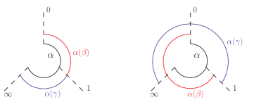
Figure 7: The two possibilities for three way boundary matching. We plot the range of $\alpha$ on a circle from $[-\infty,\infty]$ passing through 0 and 1. Black is the range of $\alpha$ in diagram D1, in red that of $\alpha(\beta)$ in $D_{2}$ and in blue the range of $\alpha(\gamma)$ in $D_{3}$. We see there is always a pairwise matching of the three diagrams in both cases. In Case 1 D2 and D3 each only overlap with D1 and not with each other. For Case 2 all diagrams overlap the other two.

4.2.1 Case 1: $\alpha>0$, $\beta<0$ and $\gamma<0$

Looking at Figure 7a, $C_{1}$ and $C^{\prime}_{2}$ should overlap when $0<\alpha<1$ whereas $C_{1}$ and $C^{\prime}_{3}$ should overlap when $1<\alpha<\infty$.

Now at the points where the regions overlap we also need all other variables to match. In particular this fixes the signs of the variables for the second two diagrams in terms of the first. Defining

$$\operatorname{sgn}(a_{1})=s_{1},\quad\operatorname{sgn}(b_{1})=s_{2},\quad\operatorname{sgn}(c_{1})=s_{3},$$

$$\operatorname{sgn}(d_{1})=s_{4},\quad\operatorname{sgn}(g_{1})=s_{5},\quad\operatorname{sgn}(h_{1})=s_{6}$$ (53)

Then by comparing (51,52) to (50) and undoing the $GL(2)$ transformation we must have the following signs in each entry

$$\operatorname{sgn}(C_{1})=\begin{pmatrix}s_{1}&s_{2}&s_{3}&s_{4}&0&0&1\\ 0&0&s_{3}&s_{4}&s_{5}&s_{6}&1\end{pmatrix}$$ (54)

$$\operatorname{sgn}(C_{2})=\begin{pmatrix}-s_{1}&-s_{2}&0&0&s_{5}&s_{6}&1\\ s_{1}&s_{2}&s_{3}&s_{4}&0&0&1\end{pmatrix}$$ (55)

$$\operatorname{sgn}(C_{3})=\begin{pmatrix}s_{1}&s_{2}&0&0&-s_{5}&-s_{6}&1\\ 0&0&s_{3}&s_{4}&s_{5}&s_{6}&1\end{pmatrix}.$$ (56)

Given a set of signs for $C_{1}$, the three way cancellation fixes the signs of $C_{2}$ and $C_{3}$. Although these signs are derived by looking at their values at the spurious boundary, crucially the signs remain unchanged inside the region even on moving away from the boundary.

But now the sign choices for diagrams $D_{1},D_{2},D_{3}$ (forced on us by the three way cancellation Case 1) can be seen to be inconsistent with the consecutive matching of the other type of spurious boundary where propagator ends approach vertices. The problem comes down to the difference in signs in the top row of (55) with those of (56).

Now, consider starting with diagram $D_{2}$ and moving the propagator defined by the second line in $C_{2}$ around clockwise until the diagram $D_{3}$ is reached. At each vertex we match spurious boundaries, meaning the signs of the top row (corresponding to the propagator left fixed) must remain the same. Under this sequence of moves

$$\operatorname{sgn}(C_{2})\to\begin{pmatrix}-s_{1}&-s_{2}&0&0&s_{5}&s_{6}&1\\ 0&0&s^{\prime}_{3}&s^{\prime}_{4}&s^{\prime}_{5}&s^{\prime}_{6}&1\end{pmatrix},$$ (57)

where the prime variables represent new signs not fixed in this process.

Now comparing this new matrix to $C_{3}$ (56) one can see immediately that the signs on the top row are different, regardless of what the bottom row becomes. Therefore, the signs that are found from the matching of the three-way spurious boundary are not consistent with the matching of boundaries obtained by following the propagators round the Wilson Loop polygon. The WLDs cannot be glued together to form a geometry without spurious boundaries with this choice of $\alpha$, $\beta$ and $\gamma$.

Note this argument has been illustrated for at points but clearly doesn’t depend in any key way on the number of points.

4.2.2 Case 2: $\alpha,\beta,\gamma>0$

We then consider the second possibility for having pairwise matching boundaries where $\alpha,\beta,\gamma>0$.

Looking at Figure 7b, $C_{1}$ and $C^{\prime}_{2}$ should overlap when $1<\alpha<\infty$ and $0<\beta<1$ and $C_{1}$ and $C^{\prime}_{3}$ should overlap when $0<\alpha<1$ and $0<\gamma<1$. Now there is an additional overlap between $C^{\prime}_{2}$ and $C^{\prime}_{3}$ when $1<\beta<\infty$ and $1<\gamma<\infty$.

At these overlaps the entries of the rotated matrices (50-52) must be equal. Defining the signs of the $C_{1}$ variables as previously (53) this means the signs of the entries of $C_{2}^{\prime}$ and $C_{3}^{\prime}$, must be the same as those of $C_{1}$ in the region where they overlap with $C_{1}$ (i.e. $0<\beta<1$, $0<\gamma<1$). However when $\beta,\gamma>1$ some of the entries changes sign due their dependence on $\beta$ or $\gamma$. Thus the signs of the entries of the rotated $C$ matrices are as follows:

$$\operatorname{sgn}(C_{1}):\begin{pmatrix}s_{1}&s_{2}&s_{3}&s_{4}&0&0&1\\ 0&0&s_{3}&s_{4}&s_{5}&s_{6}&1\end{pmatrix}_{0<\alpha<\infty}$$ (58)

$$\operatorname{sgn}(C^{\prime}_{2}):\begin{pmatrix}s_{1}&s_{2}&s_{3}&s_{4}&0&0&1\\ 0&0&s_{3}&s_{4}&s_{5}&s_{6}&1\end{pmatrix}_{0<\beta<1},\begin{pmatrix}s_{1}&s_{2}&s_{3}&s_{4}&0&0&1\\ 0&0&-s_{3}&-s_{4}&-s_{5}&-s_{6}&1\end{pmatrix}_{1<\beta<\infty}$$ (59)

$$\operatorname{sgn}(C^{\prime}_{3}):\begin{pmatrix}s_{1}&s_{2}&s_{3}&s_{4}&0&0&1\\ 0&0&s_{3}&s_{4}&s_{5}&s_{6}&1\end{pmatrix}_{0<\gamma<1},\begin{pmatrix}-s_{1}&-s_{2}&-s_{3}&-s_{4}&0&0&1\\ 0&0&s_{3}&s_{4}&s_{5}&s_{6}&1\end{pmatrix}_{1<\gamma<\infty}.$$ (60)

But now there is a clear problem. Looking at the matrices for $1<\beta<\infty$ and $1<\gamma<\infty$, it can be seen they do not match as they should. Matching diagram $D_{2}$ with $D_{1}$ correctly and $D_{3}$ with $D_{1}$ correctly fixes the signs of $D_{2},D_{3}$ in a way incompatible with $D_{2}$ and $D_{3}$ matching.

Thus there is in fact no valid three way boundary matching for this case.

5 Conclusion

We have shown that surprisingly it is not possible to consistently assign a subspace of $\text{Gr}(k,k+4)$ (amplituhedron space) to each WLD consistent with its canonical form and pairwise matching of all spurious boundaries. In other words WLDs can not be used to tessellate the amplituhedron or any other shape without spurious boundaries. This despite their promising properties: WLDs do have natural (but non-unique) interpretations as subspaces in $\text{Gr}(k,k+4)$ and they do sum up to give the amplitude. The situation is similar to the example in Figure 1b where we see an attempted tessellation of the quadrilateral: although the canonical forms of the two triangles sum to the corresponding canonical forms of the quadrilateral, this is clearly not a tessellation of the quadrilateral and there are left over unmatched spurious boundaries. Of course for the quadrilateral we could choose a more sensible tessellation with matched spurious boundaries, for WLDs we have shown there is no such sensible tessellation possible.

Note that we have shown this for the N²MHV case and illustrated for six points only. We have already mentioned that the proof does not depend on the number of points. It is also clear that the proof goes through in the same way for higher MHV degree: just add another propagator somewhere away from the three way cancellation and recycle the same argument given here. We have also here focussed on tree level but it would be very surprising if moving to loop level improves the situation.

One might hope that although the WLDs do not tessellate the amplituhedron they may instead give a nice tessellation of the squared amplituhedron [18, 19] which has a more direct definition and for which there are $2^{k}$ copies of most diagrams, which could conceivably provide a way out of the problems found here. However this also seems not to be the case (although the proof is more involved and we omit it here).

We should emphasise that despite the fact that the WLDs can not provide a geometric tessellation of the amplituhedron, they do still give a very concrete and suggestive “tessellation” at the level of its canonical form. It seems likely that this property generalises for more general positive Grassmannians and may prove useful in their further mathematical study.

Acknowledgements

PH would like to thank Lionel Mason for many invaluable discussions on topics related to this. PH and AS would also like to thank Susama Agarwala and other members of the WLD virtual seminar series for the interesting seminars and discussions. AS is supported by an STFC studentship and PH acknowledges support from STFC grant ST/P000371/1.

References

- [1] A. Hodges, “Eliminating spurious poles from gauge-theoretic amplitudes,” JHEP 1305 (2013) 135 doi:10.1007/JHEP05(2013)135 [arXiv:0905.1473 [hep-th]].
- [2] N. Arkani-Hamed, J. L. Bourjaily, F. Cachazo, A. Hodges and J. Trnka, “A Note on Polytopes for Scattering Amplitudes,” JHEP 1204 (2012) 081 doi:10.1007/JHEP04(2012)081 [arXiv:1012.6030 [hep-th]].
- [3] N. Arkani-Hamed and J. Trnka, “The Amplituhedron,” JHEP 1410 (2014) 030 doi:10.1007/JHEP10(2014)030 [arXiv:1312.2007 [hep-th]].
- [4] N. Arkani-Hamed and J. Trnka, “Into the Amplituhedron,” JHEP 1412 (2014) 182 doi:10.1007/JHEP12(2014)182 [arXiv:1312.7878 [hep-th]].
- [5] Y. Bai and S. He, “The Amplituhedron from Momentum Twistor Diagrams,” JHEP 1502 (2015) 065 doi:10.1007/JHEP02(2015)065 [arXiv:1408.2459 [hep-th]].
- [6] S. Franco, D. Galloni, A. Mariotti and J. Trnka, “Anatomy of the Amplituhedron,” JHEP 1503 (2015) 128 doi:10.1007/JHEP03(2015)128 [arXiv:1408.3410 [hep-th]].
- [7] T. Lam, “Amplituhedron cells and Stanley symmetric functions,” Commun. Math. Phys. 343 (2016) no.3, 1025 doi:10.1007/s00220-016-2602-2 [arXiv:1408.5531 [math.AG]].
- [8] N. Arkani-Hamed, A. Hodges and J. Trnka, “Positive Amplitudes In The Amplituhedron,” JHEP 1508 (2015) 030 doi:10.1007/JHEP08(2015)030 [arXiv:1412.8478 [hep-th]].
- [9] S. Agarwala and E. Marin-Amat, Commun. Math. Phys. 350 (2017) no.2, 569 doi:10.1007/s00220-016-2659-y [arXiv:1509.06150 [math-ph]].
- [10] Y. Bai, S. He and T. Lam, “The Amplituhedron and the One-loop Grassmannian Measure,” JHEP 1601 (2016) 112 doi:10.1007/JHEP01(2016)112 [arXiv:1510.03553 [hep-th]].
- [11] L. Ferro, T. Lukowski, A. Orta and M. Parisi, “Towards the Amplituhedron Volume,” JHEP 1603 (2016) 014 doi:10.1007/JHEP03(2016)014 [arXiv:1512.04954 [hep-th]].
- [12] Z. Bern, E. Herrmann, S. Litsey, J. Stankowicz and J. Trnka, “Evidence for a Nonplanar Amplituhedron,” JHEP 1606 (2016) 098 doi:10.1007/JHEP06(2016)098 [arXiv:1512.08591 [hep-th]].
- [13] D. Galloni, “Positivity Sectors and the Amplituhedron,” arXiv:1601.02639 [hep-th].
- [14] S. N. Karp and L. K. Williams, “The m=1 amplituhedron and cyclic hyperplane arrangements,” arXiv:1608.08288 [math.CO].
- [15] T. Dennen, I. Prlina, M. Spradlin, S. Stanojevic and A. Volovich, “Landau Singularities from the Amplituhedron,” JHEP 1706 (2017) 152 doi:10.1007/JHEP06(2017)152 [arXiv:1612.02708 [hep-th]].
- [16] L. Ferro, T. Lukowski, A. Orta and M. Parisi, “Yangian symmetry for the tree amplituhedron,” J. Phys. A 50 (2017) no.29, 294005 doi:10.1088/1751-8121/aa7594 [arXiv:1612.04378 [hep-th]].
- [17] L. Ferro, T. Lukowski, A. Orta and M. Parisi, “Tree-level scattering amplitudes from the amplituhedron,” J. Phys. Conf. Ser. 841 (2017) no.1, 012037 doi:10.1088/1742-6596/841/1/012037 [arXiv:1612.06276 [hep-th]].
- [18] B. Eden, P. Heslop and L. Mason, “The Correlahedron,” JHEP 1709 (2017) 156 doi:10.1007/JHEP09(2017)156 [arXiv:1701.00453 [hep-th]].
- [19] N. Arkani-Hamed, H. Thomas and J. Trnka, “Unwinding the Amplituhedron in Binary,” JHEP 1801 (2018) 016 doi:10.1007/JHEP01(2018)016 [arXiv:1704.05069 [hep-th]].
- [20] S. N. Karp, L. K. Williams and Y. X. Zhang, arXiv:1708.09525 [math.CO].
- [21] J. Rao, “4-particle Amplituhedron at 3-loop and its Mondrian Diagrammatic Implication,” JHEP 1806 (2018) 038 doi:10.1007/JHEP06(2018)038 [arXiv:1712.09990 [hep-th]].
- [22] Y. An, Y. Li, Z. Li and J. Rao, “All-loop Mondrian Diagrammatics and 4-particle Amplituhedron,” JHEP 1806 (2018) 023 doi:10.1007/JHEP06(2018)023 [arXiv:1712.09994 [hep-th]].
- [23] N. Arkani-Hamed, P. Benincasa and A. Postnikov, “Cosmological Polytopes and the Wavefunction of the Universe,” arXiv:1709.02813 [hep-th].
- [24] N. Arkani-Hamed, Y. Bai, S. He and G. Yan, “Scattering Forms and the Positive Geometry of Kinematics, Color and the Worldsheet,” JHEP 1805 (2018) 096 doi:10.1007/JHEP05(2018)096 [arXiv:1711.09102 [hep-th]].
- [25] P. Galashin and T. Lam, “Parity duality for the amplituhedron,” arXiv:1805.00600 [math.CO].
- [26] S. Agarwala and S. Fryer, “A study in : from the geometric case book of Wilson loop diagrams and SYM ,” arXiv:1803.00958 [math.CO].
- [27] L. Ferro, T. Lukowski and M. Parisi, “Amplituhedron meets Jeffrey-Kirwan Residue,” arXiv:1805.01301 [hep-th].
- [28] J. Rao, “4-particle Amplituhedronics for 3-5 loops,” arXiv:1806.01765 [hep-th].
- [29] J. Bourjaily and H. Thomas, “What is the Amplituhedron?,” Not. Amer. Math. Soc. 65 (2018) no.2, 167. doi:10.1090/noti1630
- [30] N. Arkani-Hamed, Y. Bai and T. Lam, “Positive Geometries and Canonical Forms,” JHEP 1711 (2017) 039 doi:10.1007/JHEP11(2017)039 [arXiv:1703.04541 [hep-th]].
- [31] S. Agarwala and C. Marcott, “Wilson loops in SYM N=4 do not parametrize an orientable space,” arXiv:1807.05397 [math-ph].
- [32] L. J. Mason and D. Skinner, “The Complete Planar S-matrix of N=4 SYM as a Wilson Loop in Twistor Space,” JHEP 1012 (2010) 018 doi:10.1007/JHEP12(2010)018 [arXiv:1009.2225 [hep-th]].
- [33] D. Chicherin and E. Sokatchev, JHEP 1702 (2017) 062 doi:10.1007/JHEP02(2017)062 [arXiv:1601.06803 [hep-th]].
- [34] D. Chicherin, P. Heslop, G. P. Korchemsky and E. Sokatchev, “Wilson Loop Form Factors: A New Duality,” JHEP 1804 (2018) 029 doi:10.1007/JHEP04(2018)029 [arXiv:1612.05197 [hep-th]].
- [35] L. F. Alday and J. M. Maldacena, “Gluon scattering amplitudes at strong coupling,” JHEP 0706 (2007) 064 doi:10.1088/1126-6708/2007/06/064 [arXiv:0705.0303 [hep-th]].
- [36] J. M. Drummond, G. P. Korchemsky and E. Sokatchev, “Conformal properties of four-gluon planar amplitudes and Wilson loops,” Nucl. Phys. B 795 (2008) 385 doi:10.1016/j.nuclphysb.2007.11.041 [arXiv:0707.0243 [hep-th]].
- [37] A. Brandhuber, P. Heslop and G. Travaglini, “MHV amplitudes in N=4 super Yang-Mills and Wilson loops,” Nucl. Phys. B 794 (2008) 231 doi:10.1016/j.nuclphysb.2007.11.002 [arXiv:0707.1153 [hep-th]].
- [38] D. Chicherin, R. Doobary, B. Eden, P. Heslop, G. P. Korchemsky, L. Mason and E. Sokatchev, “Correlation functions of the chiral stress-tensor multiplet in SYM,” JHEP 1506 (2015) 198 doi:10.1007/JHEP06(2015)198 [arXiv:1412.8718 [hep-th]].