Understanding the Local Flow Rate Peak of a Hopper Discharging Discs through an Obstacle Using a Tetris-like Model

Abstract

Placing a round obstacle above the orifice of a flat hopper discharging uniform frictional discs has been experimentally and numerically shown in the literature to create a local peak in the gravity-driven hopper flow rate. Using frictionless molecular dynamics (MD) simulations, we show that the local peak is unrelated to the interparticle friction, the particle dispersity, and the obstacle geometry. We then construct a probabilistic Tetris-like model, where particles update their positions according to prescribed rules rather than in response to forces, and show that Newtonian dynamics are also not responsible for the local peak. Finally, we propose that the local peak is caused by an interplay between the flow rate around the obstacle, greater than the maximum when the hopper contains no obstacle, and a slow response time, allowing the overflowing particles to converge well upon reaching the hopper orifice.

I Introduction

Placing a round obstacle near the orifice of a granular hopper has recently been shown to reduce particle clogging Zuriguel et al. (2011, 2014); Endo et al. (2018) and locally speed up the gravity-driven hopper flow rate Zuriguel et al. (2011); Lozano et al. (2012); Alonso-Marroquin et al. (2012); Pastor et al. (2015); Murray and Alonso-Marroquin (2016). The flow rate exhibits a peak as the obstacle is placed an optimal distance away from the orifice of the hopper. Intrigued by these findings, we want to understand what role interparticle friction, particle size dispersity, obstacle geometry, and the Newtonian dynamics that produce interparticle cooperative motion plays in the appearance of a flow rate peak.

To study the role of interparticle friction, we use a molecular dynamics (MD) method to simulate frictionless, monodisperse discs flowing about a round obstacle placed near the orifice of a hopper. We measure the gravity-driven flow rate $J_{a}$ in terms of number of discs out of the hopper per unit time. Interestingly, eliminating friction in the system does not prevent the local flow rate peak from occurring even though the peak value, normalized by the flow rate $J_{o}$ when the hopper contains no obstacle, becomes smaller than unity. Changing particle dispersity from monodisperse to bidisperse or altering the obstacle shape from round to nearly flat also does not annihilate the local peak. The MD results suggest that interparticle friction, particle dispersity, and obstacle geometry are not fundamental factors responsible for the hopper flow rate peak. We therefore propose a necessary condition for predicting the occurrence of the flow rate peak: the peak should appear soon after the flow rate $J_{i}$ measured at the obstacle becomes greater than $J_{o}$. This condition approximately forecasts where the local flow rate peak happens without resorting to the continuum theory of granular hopper flow. We successfully verify the proposed necessary condition, $J_{i}/J_{o}>1$, using frictionless MD simulations.

In light of our MD results, we further reduce the dynamics of the system by completely switching off Newton’s equations of motion through the introduction of a Tetris-like model. Circular particles of equal size in a hopper update their positions sequentially under a set of prescribed rules, similar to the classical video game Tetris, forming a probability-driven hopper flow with adjustable driving strength. Another identically-named but more simplified model has been used to study the compaction of granular materials under vibration Caglioti et al. (1997). In the Tetris-like model, particles interact with their nearest neighbors by means of trial-and-error position-update cycles. The model maintains the essential dynamics of granular materials through non-overlap geometrical constraints, which occasionally creates particle clogging. The lack of Newtonian dynamics in the Tetris-like model inherently suspends interparticle cooperative motion via forces. Surprisingly, we can observe the local flow rate peak so long as the necessary condition $J_{i}/J_{o}>1$ is satisfied and a slow response time explained below even in this probabilistic model with minimal dynamics, and the maximum value of the normalized local flow rate peak $J_{a}/J_{o}$ can be below or above unity, similar to the results reported in studies using inanimate frictionless or frictional objects, or even animals Garcimartín et al. (2015); Zuriguel et al. (2016).

Based on the results of the Tetris-like model, we suggest that the local flow rate peak can be qualitatively understood by combining a linearly increasing $J_{i}$, satisfying the necessary condition $J_{i}/J_{o}>1$, and a slow response time, restricting the flow rate of particles passing the obstacle to reaching the hopper orifice. The slow response time allows discharged particles to merge more fully as they move towards the hopper orifice, resulting in the merged particles having a packing density high enough to show a local peak of $J_{a}/J_{o}$ as long as the obstacle is placed at some optimal height. We expect that a slower response time corresponds to a larger variation in the number of times a particle fails to update its position, $n_{hit}$, as a function of obstacle location. We observe the expected relation in representative cases showing local flow rate peaks, and verify our idea successfully.

Below we elaborate on our Tetris-like model which generates the probability-driven hopper flow in section II, followed by quantitative investigation of the hopper flow rates in section III. Finally, we conclude our study in section IV. Since we focus on the Tetris-like model in the main text, we leave the description of our frictionless MD simulations to the appendix section VII for reference.

II The Tetris-like model

To study the externally-driven granular hopper flow without the involvement of Newtonian dynamics, we propose a purely geometrical Tetris-like model. Tetris is a classic video game where solid objects with given shapes drop down one by one towards the bottom of the playing field. The player can shift the objects horizontally at will during the dropping process. In our Tetris-like model, each circular particle $i$ of equal diameter $d$ has exactly one chance per position-update cycle to change its horizontal ($x$) and vertical ($y$) positions from $(x_{i}^{old},y_{i}^{old})$ to $(x_{i}^{new},y_{i}^{new})$ , according to

$$x_{i}^{new}={N_{x}}(x_{i}^{old},\sigma),$$ (1)

and

$$y_{i}^{new}=\left|{{N_{y}}(y_{i}^{old},\alpha\sigma)}\right|,$$ (2)

where $N_{x}$ and $N_{y}$ are two independent Gaussian functions. $N_{x}$ has a mean at $x_{i}^{old}$ and a standard deviation $\sigma$, while $N_{y}$ has a mean at $y_{i}^{old}$ and a standard deviation $\alpha\sigma$, as shown schematically in Fig.1(a). The absolute value about $N_{y}$ forbids backward movements of particles. We choose $\sigma=0.05d$ throughout this study, and $\alpha$ is a control parameter representing the strength of driving particles towards the orifice of the hopper, similar to the driving force of discharging animate or inanimate particles through constrictions Pastor et al. (2015).

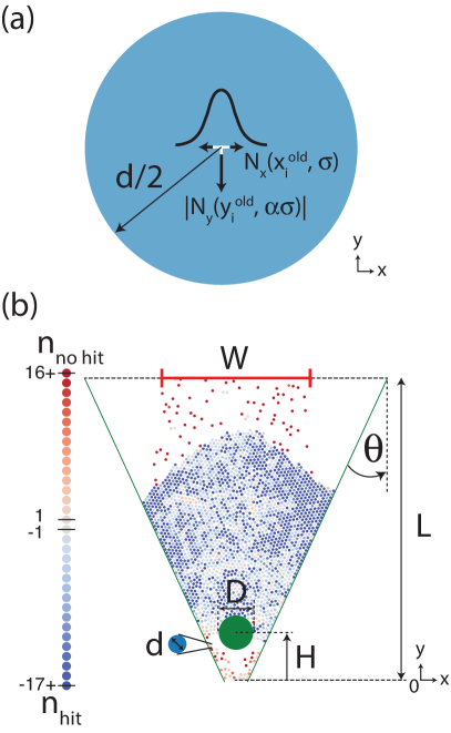
Figure 1: (Color online) (a) The objects of the Tetris-like model are demonstrated by the disc particle of diameter $d$ (blue circle). The particle’s next position is governed by two independent Gaussian functions, $N_{x}$ and $N_{y}$ having (mean, standard deviation) equal to ($x_{i}^{old},\sigma$) and ($y_{i}^{old},\alpha\sigma$), respectively. $\sigma=0.05d$ and $\alpha$ is a variable of the driving strength in this study. (b) The simulation setup of a symmetric hopper (green lines) with equal height and top-width $L$, and a hopper angle $\theta$. An obstacle (green circle) of diameter $D$ is located at a height $H$ above the hopper orifice. The hopper discharges particles, colored by $n_{no\ hit}$ or $n_{hit}$ recording the history of successfully or unsuccessfully updating their positions successively in a linear scale. The discharged particles reenter the hopper from its top border within $W=0.5L$ through a random dispersion. The snapshot is taken with $\alpha=0.128$.

There are $N=2048$ randomly placed particles in the hopper in the beginning of a simulation, and we update their positions sequentially using a random list, renewed repetitively per position-update cycle. The Tetris-like model accepts a position update of a particle if it creates no overlap with any other objects in the system. A positive parameter $n_{no\ hit}$, starting from zero, is increased by one to save this successful trial. Otherwise, the update is rejected and the particle stays still. Similarly, a negative parameter $n_{hit}$, also starting from zero, is decreased by one to save this failed trial. $n_{no\ hit}$ is reset when $n_{hit}$ becomes nonzero, and vice versa. The hopper is geometrically symmetric and has a height $L=83d$ and a hopper angle $\theta=0.4325$ radians. A circular obstacle of diameter $D=0.112L$ and $D/d=9.296$ is placed along the symmetric axis of the hopper a height $H$ above its orifice. To maintain a constant $N$, a particle leaving the hopper will reenter it from its top border with the particle’s $x$ position randomly reassigned within a range $W\in[-L/4,L/4]$. A snapshot of the probability-driven hopper flow is shown in Fig.1(b). Further details about the Tetris-like model can be found in our previous study Gao (2018).

Using the Tetris-like model, we measure the actual flow rate $J_{a}$ in terms of the average number of particles passing the hopper orifice per position-update cycle, and define $J_{o}$ as the value of $J_{a}$ while the hopper contains no obstacle. We also measure the average number of particles $J_{i}$ flowing out of the two channels between the obstacle and the hopper walls, essentially considering the flow rate of an imperfect hopper with the part of its orifice lower than the center of the obstacle removed. Our Tetris-like model sometimes encounters persistent clogging events due to geometrical particle arching, as shown by the explanatory snapshots in Fig.2. These events exist within a completely different timescale. This issue becomes serious when the driving strength $\alpha$ is very weak, similar to extremely slow grain velocities cause orders of magnitude higher hopper clogging probability found in experiments Gella et al. (2018). To ensure that measured flow rates are free from persistent clogging events we discard simulation data containing clogging events lasting longer than $10,000$ position-update cycles, a practice similar to using vibration to resume the clogged hopper flow in experiments Pastor et al. (2015).

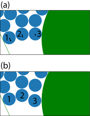
Figure 2: (Color online) Snapshots of an arch forming and breaking event in the Tetris-like model with $\alpha=1.0$. (a) Particles 1, 2, and 3 form the arch. The arrows on the particles indicate the minimal jump distance for escaping from the geometrical constraint without creating any overlap with their neighboring particles. (b) The arch breaks when particle 3, having the shortest jump distance for escaping and therefore the highest chance of success, is the first to undermine the arch.

III Results and Discussions

Below, we show the normalized hopper flow rates $J_{a}/J_{o}$ as a function of the driving strength $\alpha$. We then focus on two exemplary cases: $\alpha=0.333$ showing a local flow rate peak and $\alpha=0.439$ showing no peak. Finally, we offer a plausible mechanism for the observed peaks backed by our simulation evidence.

III.1 The effect of the driving strength $\alpha$ on the hopper flow rate

To test the effect of the driving strength $\alpha$ on the normalized hopper flow rate $J_{a}/J_{o}$, we tried six different values of $\alpha$ between $0.062$ and $0.439$ and measured the corresponding $J_{a}/J_{o}$. The results are shown in Fig.3. We can see that when the driving strength is weak ($\alpha=0.062$ and $0.083$), $J_{a}/J_{o}$ exhibits a mild local peak below unity as the obstacle is placed around $H/d=13.5$. A similar phenomenon has been found using frictionless MD simulations, shown in Fig. 8 in the appendix section VII.4. When we increase $\alpha$ to $0.128$ and $0.222$, the local peak value of $J_{a}/J_{o}$ increases to greater than unity; the peak value of $J_{a}/J_{o}$ decreases slightly as $\alpha$ becomes $0.333$. Similar enhanced flow rates have been reported using frictional MD simulations in the literature Alonso-Marroquin et al. (2012). Finally, when we increase $\alpha$ to $0.439$, the local peak disappears and $J_{a}/J_{o}$ becomes a monotonically increasing function of $H/d$, consistent with the findings of another experimental study Endo and Katsuragi (2017).

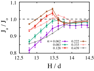
Figure 3: (Color online) Hopper flow rates $J_{a}$ measured at the hopper orifice with $\alpha=0.062$ (purple), $0.083$ (green), $0.128$ (red), $0.222$ (brown), $0.333$ (pink), and $0.439$ (grey), respectively. The error bars of each curve are obtained using $45$ different initial conditions.

III.2 Examining the hopper flow rate with or without a local peak

We take a closer look at two representative cases to learn more about what happens when a local peak in $J_{a}/J_{o}$ is shown or not shown: $\alpha=0.333$ and $0.439$, respectively.

In Fig. 4(a), we plot $J_{a}/J_{o}$, the normalized flow rate leaving the hopper orifice, and $J_{i}/J_{o}$, the normalized flow rate measured at the obstacle, as a function of $H/d$ when $\alpha=0.333$. We can see clearly that $J_{a}/J_{o}$ exhibits a local peak around $H/d=13.6$ after $J_{i}/J_{o}$ becomes greater than unity around $H/d=11.1$, which shows that $J_{i}/J_{o}>1$ is a necessary condition for a local flow rate peak of $J_{a}/J_{o}$.

We then calculate the time lapse $\Delta t$ between the egress of two consecutive particles leaving the hopper at position-update cycles $i$ and $i+\Delta t$. From the $\Delta t$ data, we plot the complementary cumulative distribution function $P(\Delta t\geq\tau)$, which gives the probability of finding a time lapse $\Delta t$ equal to or larger than $\tau$ Zuriguel et al. (2014); Pastor et al. (2015). For a given value of $H/d$, we build $P(\Delta t\geq\tau)$ using $990,000$ position-update cycles. It is possible for two or more particles to leave the hopper during the same position-update cycle, but we treat this as a single egress event and obtain only one $\Delta t$ from it. The multi-particle egress is rare and accounts for less than $1\%$ of the total egress events in the data reported here.

Fig. 4(b1-b3) show $P(\Delta t\geq\tau)$ in three continuous ranges of $H/d$, where $J_{a}/J_{o}$ first increases (Range A-B-C), then decreases (Range C-D-E), and finally reaches a steady value (Range E-F-G-H) under the mild driving strength $\alpha=0.333$. In Range A-B-C with a moderate $J_{i}/J_{o}>1$, the mild driving strength allows the two groups of particles, discharged from the two sides of the obstacle toward the center of the hopper orifice through a narrowing passage, to merge more efficiently by means of non-overlapping particle position-updates without hitting the hopper walls too often. As a result, we observe an increasing $J_{a}/J_{o}$, and upon reaching the hopper orifice, the concentration of confluent particles can be high enough to deliver a $J_{a}/J_{o}>1$ if we place the obstacle at the optimal height C, as shown by the A-B-C series of reducing $P(\Delta t\geq\tau)$ in Fig. 4(b1). However, in Range C-D-E with a stronger $J_{i}/J_{o}>1$, the clogging effect appears, shown by the C-D-E series of increasing $P(\Delta t\geq\tau)$ in Fig. 4(b2). The overall effect is a decreasing $J_{a}/J_{o}$. Lastly, in Range E-F-G-H, because the obstacle is located far from the hopper orifice, its influence on the flow rate becomes negligible, and the E-F-G-H series of $P(\Delta t\geq\tau)$ shows no clear trend, as can be seen in Fig. 4(b3).

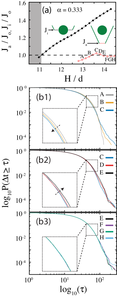
Figure 4: (Color online) (a) Hopper flow rates $J_{i}$ measured at the obstacle height (black dotted line with diamonds) and $J_{a}$ measured at the hopper orifice (pink solid line with circles) with $\alpha=0.333$. The error bars of $J_{i}$ and $J_{a}$ are obtained using $13$ and $45$ different initial conditions, respectively. The fluidized flow regime, where $J_{i}<J_{o}$, is shaded. (b1), (b2) and (b3) show representative $P(\Delta t\geq\tau)$, zoomed in the dashed boxes, using log-10 scales for both axes within three continuous ranges, A-B-C, C-D-E, and E-F-G-H, on the $J_{a}$ curve.

Similarly, in Fig. 5(a), we plot $J_{a}/J_{o}$ which exhibits no local peak under the strong driving strength $\alpha=0.439$, and the corresponding $J_{i}/J_{o}$ as a function of $H/d$. Fig. 5(b1-b3) show the related $P(\Delta t\geq\tau)$ in the same three ranges of $H/d$ as before. Unlike the milder driving strength $\alpha=0.333$, where $J_{a}/J_{o}$ can be greater than unity, discharged particles prompted by the stronger driving strength $\alpha=0.439$ block one another and hit the hopper walls more often, which on average gives a higher $n_{hit}$ per particle, resulting in less efficient merging on the way toward the hopper orifice and stagnation in the Tetris-like hopper. We can still observe an increasing $J_{a}/J_{o}$, as shown by the A-B-C series of reducing $P(\Delta t\geq\tau)$ in Fig. 5(b1); however, the concentration of confluent particles can never deliver a $J_{a}/J_{o}>1$. Due to $J_{a}/J_{o}$ remaining lower than unity, in the following range we do not observe a substantial counteractive clogging effect as in Fig. 4(b2), and $P(\Delta t\geq\tau)$ keeps decreasing until it reaches a steady value, as shown in Fig. 5 (b2) and (b3), respectively.

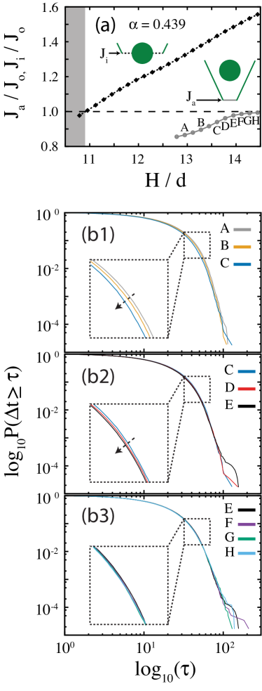
Figure 5: (Color online) The same plots as Fig. 4, except $\alpha=0.439$.

III.3 An explanation for the local flow rate peak

In our previous work Gao (2018), we suggest that ${J_{a}}\sim{{{J_{i}}}\mathord{\left/{\vphantom{{{J_{i}}}{{P_{c}}}}}\right.\kern-1.2pt}{{P_{c}}}}$, where $P_{c}$ is the probability of particle clogging below the obstacle. Reasonably, the flow rate leaving the hopper $J_{a}$ should be proportional to $J_{i}$, measuring the number of particles released from the two passages between the obstacle and the hopper walls. As $J_{i}$ increases with higher placement of the obstacle, more particles comes out from the passages. As a result, the clogging probability $P_{c}$ should also become higher, a reasoning consistent with studies claiming that the probability for a given particle to be able to participate in a clog is constant in granular hopper flow Thomas and Durian (2013, 2015). Besides, we also assume that the increasing $P_{c}$ puts a strong constraint on the value of $J_{a}$.

In this study, we explicitly show in Fig. 4(a) and Fig. 5(a) that $J_{i}$ is a linear function of $H/d$ obtained by discarding data of $J_{i}$ containing clogging events in the Tetris-like model, as discussed in section II and shown in Fig.2. In addition, we assume that $P_{c}$ is proportional to the absolute value of $n_{hit}$, defined as a negative number recording how many times a particle fails to update its position due to creating an overlap with other objects in the hopper, that is, ${P_{c}}\sim\left|{{n_{hit}}}\right|$. Using only the $n_{hit}$ data of particles whose positions are below the obstacle, we build its complementary cumulative distribution function $P(\left|{{n_{hit}}}\right|\geq\nu)$, which gives the probability of finding a particle failing to move equal to or larger than $\nu$ times. The results of $P(\left|{{n_{hit}}}\right|\geq\nu)$ for $\alpha=0.333$ and $\alpha=0.439$, covering the same three ranges of $H/d$ discussed in Fig. 4 and Fig. 5, are shown in Fig. 6.

In Fig. 6(a) with the weaker driving strength $\alpha=0.333$, we can see that the variation of $P(\left|{{n_{hit}}}\right|\geq\nu)$ is larger. This indicates a slower response time of the system, once it senses an increasing supply of particles $J_{i}$ in the upper stream and tries to regulate the output flow rate $J_{a}$ by increasing $n_{hit}$. In the inset, we schematically draw ${J_{a}}\sim{J_{i}}\times\frac{1}{{{P_{c}}}}$. A linearly increasing $J_{i}$ and a steep ${1\mathord{\left/{\vphantom{1{{P_{c}}}}}\right.\kern-1.2pt}{{P_{c}}}}\sim{1\mathord{\left/{\vphantom{1{\left|{{n_{hit}}}\right|}}}\right.\kern-1.2pt}{\left|{{n_{hit}}}\right|}}$ presumably can allow $J_{a}$ to overshoot briefly and exhibit a local peak, as observed in our simulation results and reported in other experimental and numerical studies. In the literature Zuriguel et al. (2011), it has been claimed that an effective pressure reduction in the region of arch formation below the obstacle and above the orifice can explain the local hopper flow rate peak. However, in the Tetris-like model where force and pressure are undefined, we can still see the local flow rate peak; our explanation offers a novel point of view.

On the other hand, if the driving strength is stronger, the response time of the system becomes faster and, therefore, the variation in $P(\left|{{n_{hit}}}\right|\geq\nu)$ is smaller, as shown in Fig. 6(b). In its inset, the nearly flat ${1\mathord{\left/{\vphantom{1{{P_{c}}}}}\right.\kern-1.2pt}{{P_{c}}}}\sim{1\mathord{\left/{\vphantom{1{\left|{{n_{hit}}}\right|}}}\right.\kern-1.2pt}{\left|{{n_{hit}}}\right|}}$ restricts $J_{a}$ from having a local peak. We will pursue the functional form of ${J_{a}}\sim{{{J_{i}}}\mathord{\left/{\vphantom{{{J_{i}}}{\left|{{n_{hit}}}\right|}}}\right.\kern-1.2pt}{\left|{{n_{hit}}}\right|}}$ in future work.

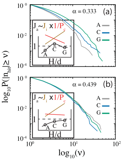
Figure 6: (Color online) Representative $P(\left|{{n_{hit}}}\right|\geq\nu)$, using log-10 scales for both axes, across a range of A-C-G on the $J_{a}$ curves of (a) $\alpha=0.333$ and (b) $\alpha=0.439$ as in Fig. 4(a) and Fig. 5(a), respectively. The insets show schematically drawn ${J_{a}}\sim{J_{i}}\times\frac{1}{{{P_{c}}}}$, where $J_{i}$ (brown) are alike, but $1/P_{c}$ (red) is steeper in (a), where the driving strength $\alpha$ is weaker, and allows a local peak of the hopper flow $J_{a}$.

IV Conclusions

Using frictionless MD simulations, we show that the interparticle friction, obstacle geometry, and particle dispersity have no fundamental contribution to the occurrence of a local peak in the actual hopper flow rate $J_{a}$, as recently reported in frictional systems with discs passing about a round obstacle Alonso-Marroquin et al. (2012). Guided by our frictionless MD results, we suggest a necessary condition, $J_{i}/J_{o}>1$, for observing the local peak, formulated in terms of the flow rate $J_{i}$ measured at the obstacle and the maximum flow rate $J_{o}$ at the orifice when the hopper contains no obstacle. Our evidence from frictionless MD simulations supports the proposed necessary condition well.

While the necessary condition identifies when one can expect a local flow rate peak to happen, it does not explain the reason behind it. The local effect is still perplexed by factors such as the interparticle collaborative motion that emerges from the Newtonian dynamics. For example, a group of particles can crystallize above the obstacle or there could be coordinated motions between particles below the obstacle before they leave the hopper. To reveal the fundamental cause for the focused phenomenon we proposed a Tetris-like model to reduce the dynamics of the system to its bare-bones minimum. In this model, particles moved sequentially according to prescribed probability functions without any communication through Newton’s equations of motion, creating an artificial probability-driven hopper flow. The non-overlap position-update procedure in the model allows particles to clog. Strikingly, the peak of $J_{a}$ still occurs. This serves as indisputable evidence that the Newtonian dynamics and associated interparticle collaborative motion are not essential for this local phenomenon.

Enlightened by the results of our Tetris-like model, we devise a mechanism to explain the local flow rate peak by introducing a response time that uses detection of $J_{i}/J_{o}>1$ to restrict flow rate $J_{a}$ exiting the hopper. The mechanism utilizes the dependence of $J_{a}$ on the linearly increasing flow rate $J_{i}$ and the effect of the hopper below the obstacle. As $J_{a}$ is regulated within the response time, the particles below the obstacle rearrange themselves, subject to the non-overlap condition, as they move toward the hopper orifice. If the necessary condition $J_{i}/J_{o}>1$ is satisfied and the response time is slower, the two groups of particles discharged from the two passages between the obstacle and the hopper wall can merge better. This promotes a higher packing density at the hopper orifice, allowing the local peak of $J_{a}/J_{o}$ to be possible. We link a slower response time with a larger variation in the clogging probability $P_{c}$ within the space between the obstacle and the hopper orifice. $P_{c}$ is quantified by measuring the number of times a particle fails to update its position, $n_{hit}$, as a function of the obstacle location. For representative cases where $J_{a}/J_{o}$ exhibits a local peak, we do observe the expected large variations in $n_{hit}$; however, for cases showing no local peak of $J_{a}/J_{o}$, the variations become reasonably small. In this, we indirectly verify the proposed mechanism. Our Tetris-like model offers an example of how one can elucidate underlying mechanisms of a complicated local phenomenon in an athermal granular system using a simplified model that preserves only the essential dynamics.

V acknowledgments

GJG gratefully acknowledges financial support from startup funding of Shizuoka University (Japan).

VI Compliance with ethical standards

Conflict of Interest: The authors declare that they have no conflict of interest. The research presented did not involve human participants and/or animals.

VII Appendix: Frictionless MD simulations

VII.1 System geometry

In our MD simulations studying the gravity-driven discharging of monodisperse or 50-50 bidisperse frictionless circular dry particles, shown schematically in Fig.7, the hopper and the obstacle have the same geometry as in the Tetris-like model. The obstacle could be one disc of diameter $D$ or three horizontally-aligned discs, each of diameter $D/3$ to resemble a flat obstacle. The disc diameter $d$ of the monodisperse system is about the same as the large disc diameter $d_{l}$ of the bidisperse system, with $L/d=83$ and $L/d_{l}=82.857$. The size ratio between the obstacle and a particle is $D/d=9.296$ and $D/d_{l}=9.28$. In the bidisperse system, the diameter ratio between large and small discs is $d_{l}/d_{s}=1.4$ to prevent artificial crystallization in a two dimensional environment. There are $N$ discs in the system, where $N=2048$ and $2712$ for the monodisperse and bidisperse systems, respectively. These values ensure that the particles in each system only fill the hopper up to about $2/3$ of its height while a steady hopper flow is maintained. To maintain a constant number of particles $N$ in our hopper flow simulation, a particle dropping out of the hopper will reenter it from its top border by artificially shifting the particle’s vertical (y) position by a distance $L$ while keeping its horizontal (x) position and velocities in both directions unchanged.

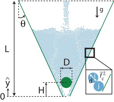
Figure 7: (Color online) The MD simulation setup modeling steady gravity-driven hopper flow of frictionless discs (blue circles) of diameter $d$. An obstacle (green circle) of diameter $D$ sits at a height $H$ above the orifice of a symmetric hopper (green straight lines) with a height $L$ and a hopper angle $\theta$. Gravity $g$ is in the downward (-y) direction. The inset shows that the discs are subject to interparticle normal forces only.

VII.2 Interactions between objects within the system

In our MD simulation, initially orderly placed discs fall under gravity and the system eventually reaches a steady state to form a gravity-driven hopper flow. Each particle $i$ obeys Newton’s translational equation of motion

$${{\mathord{\buildrel{\lower 3.0pt\hbox{$\scriptscriptstyle\rightharpoonup$}}\over{F}}}_{i}}=\mathord{\buildrel{\lower 3.0pt\hbox{$\scriptscriptstyle\rightharpoonup$}}\over{F}}_{i}^{{\mathop{\rm int}}}+\mathord{\buildrel{\lower 3.0pt\hbox{$\scriptscriptstyle\rightharpoonup$}}\over{F}}_{i}^{W}+\mathord{\buildrel{\lower 3.0pt\hbox{$\scriptscriptstyle\rightharpoonup$}}\over{F}}_{i}^{I}+\mathord{\buildrel{\lower 3.0pt\hbox{$\scriptscriptstyle\rightharpoonup$}}\over{F}}_{i}^{G}={m_{i}}{{\mathord{\buildrel{\lower 3.0pt\hbox{$\scriptscriptstyle\rightharpoonup$}}\over{a}}}_{i}},$$ (3)

where ${{\mathord{\buildrel{\lower 3.0pt\hbox{$\scriptscriptstyle\rightharpoonup$}}\over{F}}}_{i}}$ is the total force acting on particle $i$ with mass $m_{i}$, and acceleration ${{\mathord{\buildrel{\lower 3.0pt\hbox{$\scriptscriptstyle\rightharpoonup$}}\over{a}}}_{i}}$. $\mathord{\buildrel{\lower 3.0pt\hbox{$\scriptscriptstyle\rightharpoonup$}}\over{F}}_{i}^{{\mathop{\rm int}}}$, $\mathord{\buildrel{\lower 3.0pt\hbox{$\scriptscriptstyle\rightharpoonup$}}\over{F}}_{i}^{W}$, $\mathord{\buildrel{\lower 3.0pt\hbox{$\scriptscriptstyle\rightharpoonup$}}\over{F}}_{i}^{I}$ and $\mathord{\buildrel{\lower 3.0pt\hbox{$\scriptscriptstyle\rightharpoonup$}}\over{F}}_{i}^{G}$ are forces acting on particle $i$ from its contact neighbors, the hopper wall, the obstacle, and gravity, respectively.

The simplest model of frictionless granular materials considers only the interparticle normal forces Gao et al. (2009). The interparticle force $\mathord{\buildrel{\lower 3.0pt\hbox{$\scriptscriptstyle\rightharpoonup$}}\over{F}}_{i}^{{\mathop{\rm int}}}$ on particle $i$ having $N_{c}$ contact neighbors can be expressed as

$$\mathord{\buildrel{\lower 3.0pt\hbox{$\scriptscriptstyle\rightharpoonup$}}\over{F}}_{i}^{{\mathop{\rm int}}}=\sum\limits_{j\neq i}^{{N_{c}}}{[\mathord{\buildrel{\lower 3.0pt\hbox{$\scriptscriptstyle\rightharpoonup$}}\over{f}}_{ij}^{n}}({r_{ij}})+\mathord{\buildrel{\lower 3.0pt\hbox{$\scriptscriptstyle\rightharpoonup$}}\over{f}}_{ij}^{d}({r_{ij}})],$$ (4)

where $\mathord{\buildrel{\lower 3.0pt\hbox{$\scriptscriptstyle\rightharpoonup$}}\over{f}}_{ij}^{n}({r_{ij}})$ and $\mathord{\buildrel{\lower 3.0pt\hbox{$\scriptscriptstyle\rightharpoonup$}}\over{f}}_{ij}^{d}({r_{ij}})$ are the interparticle normal force and normal damping force defined below in Eqn.(5) and Eqn.(6), respectively.

Specifically, we assume that each frictionless particle $i$ is subjected to a finite-range, purely repulsive linear spring normal force from its contact neighbor $j$

$$\mathord{\buildrel{\lower 3.0pt\hbox{$\scriptscriptstyle\rightharpoonup$}}\over{f}}_{ij}^{n}({r_{ij}})=\frac{\epsilon}{{d_{ij}^{2}}}{\delta_{ij}}\Theta({\delta_{ij}}){{\hat{r}}_{ij}},$$ (5)

where $r_{ij}$ is the separation between disc particles $i$ and $j$, $\epsilon$ is the characteristic elastic energy scale, $d_{ij}=(d_{i}+d_{j})/2$ is the average diameter, $\delta_{ij}=d_{ij}-r_{ij}$ is the interparticle overlap, $\Theta(x)$ is the Heaviside step function, and ${{\hat{r}}_{ij}}$ is the unit vector connecting particle centers.

Similarly, we consider only the interparticle normal damping force proportional to the relative velocity between particles $i$ and $j$

$$\mathord{\buildrel{\lower 3.0pt\hbox{$\scriptscriptstyle\rightharpoonup$}}\over{f}}_{ij}^{d}({r_{ij}})=-b\Theta({\delta_{ij}})({{\mathord{\buildrel{\lower 3.0pt\hbox{$\scriptscriptstyle\rightharpoonup$}}\over{v}}}_{ij}}\cdot{{\hat{r}}_{ij}}){{\hat{r}}_{ij}},$$ (6)

where $b$ is the damping parameter, and ${{\mathord{\buildrel{\lower 3.0pt\hbox{$\scriptscriptstyle\rightharpoonup$}}\over{v}}}_{ij}}$ is the relative velocity between the two particles. The normal damping force results in deduction of the kinetic energy of the system after each pairwise collision.

The interaction force $\mathord{\buildrel{\lower 3.0pt\hbox{$\scriptscriptstyle\rightharpoonup$}}\over{F}}_{i}^{W}$ between particle $i$ and a hopper wall has an analogous form to the interparticle interaction $\mathord{\buildrel{\lower 3.0pt\hbox{$\scriptscriptstyle\rightharpoonup$}}\over{F}}_{i}^{{\mathop{\rm int}}}$ with $\epsilon^{W}=2\epsilon$, which means when a particle hits a wall, it experiences a repulsive force as if it hit another mirrored self on the other side of the wall. The particle-obstacle interaction force $\mathord{\buildrel{\lower 3.0pt\hbox{$\scriptscriptstyle\rightharpoonup$}}\over{F}}_{i}^{I}$ also has the same analogous form, and its value stays zero if the hopper contains no obstacle. Finally, $\mathord{\buildrel{\lower 3.0pt\hbox{$\scriptscriptstyle\rightharpoonup$}}\over{F}}_{i}^{G}=-{m_{i}}g\hat{y}$, where $g$ is the gravitational constant, and $\hat{y}$ is the unit vector in the upward direction. There is no tangential interaction on particles in this model, and therefore Newton’s rotational equation of motion is automatically satisfied.

The MD simulations in this study use the diameter $d$ and the mass $m$ of the monodisperse particles and the interparticle elastic potential amplitude $\epsilon$ as the reference length, mass, and energy scales, respectively. For the bidisperse system, the diameter $d_{s}$ and the mass $m_{s}$ of the small particles separately replace $d$ and $m$. To maintain a steady hopper flow without particles piling up to the upper border of the hopper and bringing in unwanted boundary effects, we use the dimensionless damping parameter to $b^{*}=db/\sqrt{m\epsilon}=0.5$, the dimensionless gravity $g^{*}$ to $10^{-4}$, and a dimensionless time step $dt^{*}=dt/{d}\sqrt{{m}/\epsilon}$ to $10^{-3}$ throughout this study.

VII.3 Measuring the hopper flow rate

To measure the hopper flow rate while the obstacle is placed at a given value of $H$ above the hopper orifice, we initiate one simulation with orderly arranged particles. We also randomized size identities for the bidisperse system. Then we wait for a time interval $\Delta t^{*}=5\times 10^{4}$ until the system forgets the initial arrangement and reaches a steady state to form a gravity-driven hopper flow. After that, we count the number of particles passing the orifice of the hopper within another $\Delta t^{*}$. For each value of $H$, we use 18 different initial conditions to evaluate the average and the variance of the actual flow rate $J_{a}$ in terms of number of particles leaving the hopper per unit time. We define $J_{o}$ as the value of $J_{a}$ while the hopper contains no obstacle.

VII.4 Simulation results

Our investigation contains two parts: A) To understand the influence of the interparticle friction on the locally enhanced hopper flow rate, we compare our frictionless results of the same hopper geometry with the frictional data, copied from reference Alonso-Marroquin et al. (2012), where monodisperse disc particles are passing about a round obstacle. B) To understand the contribution of the obstacle geometry or particle dispersity, we measured the flow rates of frictionless discs in three cases: (1) monodisperse discs and a round obstacle, (2) monodisperse discs and a flat obstacle, and (3) 50-50 bidisperse discs and a round obstacle. The results are shown in Fig. 8, where the actual flow rate $J_{a}$, normalized by $J_{o}$, is plotted against the normalized obstacle position $H/d$ or $H/d_{l}$ for the monodisperse or bidisperse system. $J_{o}$ is $\approx 0.0319$ for the monodisperse system, and its value increases by about $27\%$ to $\approx 0.0406$ for the bidisperse system.

Figure 8: (Color online) Averaged frictionless flow rates $J_{a}/J_{o}$ under different simulation setup: (1) monodisperse discs and a round obstacle (red); (2) monodisperse discs and a near flat obstacle (green); (3) bidisperse discs and a round obstacle (blue). The inset zooms in the dashed area. Each data point is obtained using 18 different initial conditions. A simulation snapshot of each frictionless setup is shown on the top with corresponding border color. The frictional flow rate of monodisperse discs and a round obstacle (black) is reproduced from Fig. 3(b) in Ref. Alonso-Marroquin et al. (2012) for a quantitative comparison.

VII.4.1 Comparing with the frictional data

Unlike their frictional counterparts, reproduced from reference Alonso-Marroquin et al. (2012), frictionless particles start to flow earlier and the normalized flow rate $J_{a}/J_{o}$ already reaches about $60\%$ or higher as the obstacle is lifted to about ten-particles high ($H/d\approx 10$) above the hopper orifice. On the other hand, the frictional normalized flow rate is only slightly above zero at a similar $H/d$. The local peak value of frictional $J_{a}/J_{o}$ can be greater than unity, while all three frictionless peaks have $J_{a}/J_{o}$ below unity with lower heights.

VII.4.2 Comparing between frictionless cases

We find that the normalized hopper flow rate $J_{a}/J_{o}$ exhibits a local peak in all three frictionless cases when the obstacle is lifted to about eleven to twelve particles high ($H/d\approx 11$ to $12$) above the orifice of the hopper. Among the three cases, the bidisperse one with a larger $J_{o}$ exhibits its flow rate peak at $H/d\approx 11.4$, earlier than the other two monodisperse cases. Between the two monodisperse cases with a round and a flat obstacle, the round obstacle blocks the hopper flow less than the flat one, and the system shows a peak slightly earlier at $H/d\approx 12$.

VII.4.3 An necessary condition for the local flow rate peak

Our results clearly show that none of the interparticle friction, the obstacle geometry, or the particle dispersity is directly responsible for the appearance of a local flow rate peak, though they do effectively affect its position and magnitude. To better predict when a flow rate peak occurs, we propose an indicator which is the flow rate $J_{i}$, measured at the obstacle and normalized by $J_{o}$ while the hopper contains no obstacle, as schematically shown in Fig. 9(a). Here we measure $J_{i}$ at the same vertical height where the center of the obstacle is located, that is, the height $H$ above the orifice of the hopper. Practically, we measure $J_{i}$ by cutting off the part of the hopper below the center of the obstacle so that the removed piece of hopper has no effect on $J_{i}$.

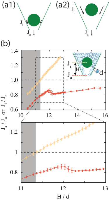
Figure 9: (Color online) (a1) Schematic defining a fluidized flow regime where the flow rate $J_{i}$ at the obstacle is smaller than the maximum $J_{o}$ when the hopper contains no obstacle. (a2) Schematic defining a clogging flow regime where $J_{i}>J_{o}$. (b) Averaged flow rates, $J_{i}$ (orange) and $J_{a}$ (red), normalized by $J_{o}$ for the frictionless system with monodisperse disc particles and a round obstacle. Each data point is obtained using 18 different initial conditions. A zoomed-in plot at the bottom emphasizes the transition from $J_{i}<J_{o}$ (fluidized flow regime, shaded) to $J_{i}>J_{o}$ (clogging flow regime, unshaded), followed by the occurrence of a local peak of $J_{a}$.

When the obstacle is located closer to the hopper orifice, $J_{i}$ is lower than $J_{o}$, defined as a fluidized flow regime as shown in Fig. 9(a1), and we should observe a monotonic increase of the actual flow rate $J_{a}$. On the other hand, when the obstacle is placed further away from the orifice, the two internal passages between the obstacle and the two hopper walls on its either side together can allow $J_{i}$ to become higher than $J_{o}$, defined as a clogging flow regime, as shown in Fig. 9(a2). Presumably, $J_{a}$ can be locally boosted in the clogging regime, due to a greater-than-unity $J_{i}/J_{o}$ that cannot be smoothly constrained by the hopper until the flow leaves its orifice, and therefore exhibits a local peak. $J_{a}$ then increases again as the position $H$ of the obstacle becomes higher until it eventually reaches its maximum $J_{o}$. We believe that $J_{i}/J_{o}>1$ is a necessary condition for observing a local flow rate peak.

To offer simulation evidence showing the proposed necessary condition is true, we plot $J_{o}$, $J_{i}$ and $J_{a}$ of the frictionless case of monodisperse discs and a round obstacle as an example. The results are shown in Fig. 9(b). To numerically measure $J_{i}$, we put particles dropping below $H$ back the top of the hopper but slightly lower than its top border by a distance of $0.1L$. Additionally, we place a lid with a dimensionless damping parameter $b^{*}_{l}=50b^{*}$ at the top border of the hopper to prevent fast-flying particles from escaping the simulation domain and conserve the total number of particles $N$ in the system. As expected, we observe a monotonic increase of $J_{a}$ while $J_{i}$ is below $J_{o}$. A peak of $J_{a}$ occurs soon after $J_{i}/J_{o}>1$, and therefore we validate the proposed necessary condition.

References

- Zuriguel et al. (2011) I. Zuriguel, A. Janda, A. Garcimartín, C. Lozano, R. Arévalo, and D. Maza, Phys. Rev. Lett. 107, 278001 (2011).
- Zuriguel et al. (2014) I. Zuriguel, D. R. Parisi, R. C. Hidalgo, C. Lozano, A. Janda, P. A. Gago, J. P. Peralta, L. M. Ferrer, L. A. Pugnaloni, E. Clément, D. Maza, I. Pagonabarraga, and A. Garcimartín, Sci. Rep. 4, 7324 (2014).
- Endo et al. (2018) K. Endo, K. A. Reddy, and H. Katsuragi, Phys. Rev. Fluids 2, 094302 (2018).
- Lozano et al. (2012) C. Lozano, A. Janda, A. Garcimartín, D. Maza, and I. Zuriguel, Phys. Rev. E 86, 031306 (2012).
- Alonso-Marroquin et al. (2012) F. Alonso-Marroquin, S. I. Azeezullah, S. A. Galindo-Torres, and L. M. Olsen-Kettle, Phys. Rev. E 85, 020301 (2012).
- Pastor et al. (2015) J. M. Pastor, A. Garcimartín, P. A. Gago, J. P. P. amd César Martín-Gómez, L. M. Ferrer, D. Maza, D. R. Parisi, L. A. Pugnaloni, and I. Zuriguel, Phys. Rev. E 92, 062817 (2015).
- Murray and Alonso-Marroquin (2016) A. Murray and F. Alonso-Marroquin, Paper in Physics 8, 080003 (2016).
- Caglioti et al. (1997) E. Caglioti, V. Loreto, H. J. Herrmann, and M. Nicodemi, Phys. Rev. Lett. 79, 1575 (1997).
- Garcimartín et al. (2015) A. Garcimartín, J. M. Pastor, L. M. Ferrer, J. J. Ramos, C. Martín-Gómez, and I. Zuriguel, Phys. Rev. E 91, 022808 (2015).
- Zuriguel et al. (2016) I. Zuriguel, J. Olivares, J. M. Pastor, C. Martín-Gómez, L. M. Ferrer, J. J. Ramos, and A. Garcimartín, Phys. Rev. E 94, 032302 (2016).
- Gao (2018) G. J. Gao, J. Phys. Soc. Jpn. 87, to appear (2018), arXiv:1807.05699.
- Gella et al. (2018) D. Gella, I. Zuriguel, and D. Maza, Phys. Rev. Lett. 121, 138001 (2018).
- Endo and Katsuragi (2017) K. Endo and H. Katsuragi, EPJ Web Conf. 140, 03004 (2017).
- Thomas and Durian (2013) C. C. Thomas and D. J. Durian, Phys. Rev. E 87, 052201 (2013).
- Thomas and Durian (2015) C. Thomas and D. Durian, Phys. Rev. Lett. 114, 178001 (2015).
- Gao et al. (2009) G. J. Gao, J. Blawzdziewicz, C. S. O’Hern, and M. D. Shattuck, Phys. Rev. E 80, 061304 (2009).