The orbital architecture and debris disks of the HR 8799 planetary system

Abstract

The HR 8799 planetary system with four $\simeq 10\,\mbox{m}_{{\mbox{\scriptsize Jup}}}$ planets in wide orbits up to $\simeq 70$ au, and orbital periods up to 500 yrs has been detected with the direct imaging. Its intriguing orbital architecture is not yet fully resolved due to time-limited astrometry covering only $\simeq 20$ years. Earlier, we constructed a heuristic model of the system based on rapid, convergent migration of the planets. Here we developed a better structured and CPU-efficient variant of this model. With the updated approach, we re-analyzed the self-consistent, homogeneous astrometric dataset in (Konopacky et al., 2016). The best-fitting configuration agrees with our earlier findings. The HR 8799 planets are likely involved in dynamically robust Laplace 8e:4d:2c:1b resonance chain. Hypothetical planets with masses below the current detection limit of 0.1-3 Jupiter masses, within the observed inner, or beyond the outer orbit, respectively, do not influence the long term stability of the system. We predict positions of such non-detected objects. The long-term stable orbital model of the observed planets helps to simulate the dynamical structure of debris disks in the system. A CPU-efficient fast indicator technique makes it possible to reveal their complex, resonant shape in $10^{6}$ particles scale. We examine the inner edge of the outer disk detected between $90$ and $145$ au. We also reconstruct the outer disk assuming that it has been influenced by convergent migration of the planets. A complex shape of the disk strongly depends on various dynamical factors, like orbits and masses of non-detected planets. It may be highly non-circular and its models are yet non-unique, regarding both observational constraints, as well as its origin.

1 Introduction

The HR 8799 planetary system has been discovered by Marois et al. (2008) as a three-planet configuration. Shortly, after two years, the fourth innermost planet has been announced by the same team (Marois et al., 2010). Since the discovery, this unusual extrasolar planetary system was studied in literally tens of papers. The parent star age, companions masses, as well as the orbital architecture and its long-term stability, debris disks, and formation are analyzed in, e.g., Read et al. (2018); Wilner et al. (2018); Wertz et al. (2017); Götberg et al. (2016); Booth et al. (2016); Konopacky et al. (2016); Contro et al. (2016); Currie (2016); Maire et al. (2015); Zurlo et al. (2016); Pueyo et al. (2015); Matthews et al. (2014); Marleau & Cumming (2014); Goździewski & Migaszewski (2014); Oppenheimer et al. (2013); Baines et al. (2012); Esposito et al. (2013); Currie et al. (2012); Sudol & Haghighipour (2012); Soummer et al. (2011); Bergfors et al. (2011); Currie et al. (2011); Galicher et al. (2011); Hinz et al. (2010); Marshall et al. (2010); Moro-Martín et al. (2010); Metchev et al. (2009); Fabrycky & Murray-Clay (2010); Lafrenière et al. (2009); Goździewski & Migaszewski (2009); Su et al. (2009); Reidemeister et al. (2009), and counting.

Regarding a characterization of the parent star and its planets, as well as the past and to date observations of debris disks in the system, we refer to the recent papers by Booth et al. (2016), Read et al. (2018), Wilner et al. (2018), and references therein. Following these works, the star is very young of $\sim 60$ Myr, within the most likely interval of 30 Myr to 160 Myr. We adopt its mass $m_{\star}$ of $1.52\,\mbox{M}_{\odot}$, and masses of the planets in the range of $5$–$10\,\,\mbox{m}_{{\mbox{\scriptsize Jup}}}$ (Marois et al., 2010).

In spite of the enormous literature on the HR 8799 system, many questions are still open. The global, orbital structure of the HR 8799 system is a particularly interesting problem. The ratio of $\simeq 120$ $(\alpha,\delta)$ measurements in the literature, collected in (Wertz et al., 2017), to 24 geometrical elements (free parameters) is 4–5 and it did not significantly change for a few past years, since the discovery of the forth companion in (Marois et al., 2010). Moreover, the major limitation of the astrometric models is a small coverage of the orbits by the measurements, between $\simeq 3\%$ and $\simeq 12\%$ for planets HR 8799b and HR 8799e, respectively, given significant uncertainties of $\simeq 10$ mas. These weak observational constraints permit a variety of non-unique orbital geometries, although all of them seem equally good fit the observations (e.g. Wertz et al., 2017; Konopacky et al., 2016).

A dynamical analysis of the best-fitting, Keplerian solutions reveal that they represent crossing orbits and configurations unstable in an enormously short 0.5–1 Myr time scale. Simple and natural requirements of the stability, like the Hill criterion, do not constrain the orbital models either, e.g., (Konopacky et al., 2016, their Fig. 3) and (Wertz et al., 2017, their Fig. B.1, especially panel for planet d). Finding long-term stable configurations simultaneously fulfilling astrometric and mass constraints is difficult even for the lower limit of the star age of 30 Myr and the low limit of the planet masses. It is still uncertain whether or not the system is strongly resonant, long-term or only marginally stable, or unstable at all (e.g., Götberg et al., 2016; Goździewski & Migaszewski, 2014, 2009; Fabrycky & Murray-Clay, 2010). It may remain a matter of somehow philosophical debate unless the orbits are observationally sampled for a sufficiently long interval of time. Furthermore, it is unclear how the system has been formed (Marois et al., 2010), given that massive planetary or brown-dwarf companions are found relatively close to the star.

Regarding dynamical arguments, none of analytic or semi-analytic criteria of stability apply to the HR 8799 system. The early dynamical studies of the three-planet system (Fabrycky & Murray-Clay, 2010; Goździewski & Migaszewski, 2009; Reidemeister et al., 2009; Marois et al., 2008) revealed that even quasi-circular and apparently wide $\simeq 70$ au orbits are separated by less than 3–4 mutual Hill radii. Such configurations are predicted as self-destructing statistically in a fraction of 1 Myr time-scale (Morrison & Kratter, 2016; Chambers et al., 1996; Chatterjee et al., 2008) unless a protecting dynamical mechanism is present. Indeed, coplanar, or close to coplanar orbits of three outer planets involved in a stable Laplace 4d:2c:1b MMR were found, explaining the astrometric observations of the HR 8799 system, shortly after its discovery (Fabrycky & Murray-Clay, 2010; Goździewski & Migaszewski, 2009; Reidemeister et al., 2009; Soummer et al., 2011; Marshall et al., 2010).

However, the stability problem became much harder with the fourth planet announced in (Marois et al., 2010). Even assuming a protecting MMR mechanism, the orbital parameters of long-living configurations may vary only within small limits (Goździewski & Migaszewski, 2014) or must be particularly tuned, since they are extremely chaotic and prone to tiny changes of the initial conditions and the numerical integrator scheme (Götberg et al., 2016).

Seeking for long-term stable orbits of the planets has a “practical” aspect, since they are needed for simulating debris disks in the system (Contro et al., 2016; Booth et al., 2016; Read et al., 2018; Wilner et al., 2018). The outer debris disk might be present between $\simeq 90$ au and $\simeq 450$ au. According to models of the ALMA observations in (Booth et al., 2016) and (Read et al., 2018), the inner edge of this disk should be placed at $\sim 145$ au, beyond the direct influence attributed to planet HR 8799b roughly at $\sim 90$ au. It might indicate the presence of an additional fifth planet, below the current detection limit of a few Jupiter masses. However Wilner et al. (2018) argue that combined ALMA and VLA observations with higher spatial resolution do not favour the fifth planet hypothesis, and the inner border of the disk may be detected at $\simeq 104$ au, consistent with the currently known four planet configuration. Moreover, they constrained the outermost planet mass $m_{\rm b}\simeq 6^{+7}_{-3}\,\mbox{m}_{{\mbox{\scriptsize Jup}}}$.

We note that some of the works devoted to debris disks (Booth et al., 2016; Read et al., 2018; Contro et al., 2016) made use of our best-fitting model representing the Laplace MMR chain (Goździewski & Migaszewski, 2014) which was found with observations up to the epoch of 2013. The most recent papers regarding astrometric models of the HR 8799 system based on to date observations, till epoch 2014.93, focus mostly on Keplerian solutions (Wertz et al., 2017; Konopacky et al., 2016). These best-fitting, or most likely models, in terms of the Bayesian inference, exhibit different geometries, such as non-coplanar, highly eccentric non-resonant or partly resonant orbits but have not been examined for their long-term orbital stability. Therefore such solutions are not suitable for the dynamical analysis of the debris disks.

In this work, we propose to resolve the structure of these disks with CPU efficient fast indicators, based on the maximal Lyapunov Characteristic Exponent (mLCE), instead of integrating orbits for a required full time span. For that purpose we need to construct long-term, rigorously stable orbits of the planets which are robust against small perturbations. Such stable planetary models are helpful to localize “missing” (non-detected) planets, or to investigate influence of such putative planets on the debris disks.

This paper is structured as follows. After this Introduction, Section 2 presents an update of the model of astrometric data through constraining it by the process of planetary migration. Section 3 regards the results and details of orbital architectures of the HR 8799 system derived for a self-consistent set of astrometric measurements in (Konopacky et al., 2016) made with the Keck II telescope. The results in this part support our idea of the orbital analysis, or could be at least an alternative and reasonable approach when compared with other solutions in the literature. Section 4 is for our model of debris disks based on the fast indicator technique, and we describe the results of its time-calibration with the direct numerical integrations. Simulations of yet undetected planets in the system are described in Sects. 5 and 6. We analyse the dynamical structure of the inner and outer debris disks in Sect. 5 and 7, respectively. We also investigate a scenario of the outer disk influenced by migrating planets in Sect. 8. Some apparent discrepancies between our approach and the results in the recent literature are addressed in Sect. 9. We summarize the work in Section 10.

2 The migration algorithm revisited

The phase space of mutually interacting planetary systems has a discrete, non-continuous structure (Malhotra, 1998). This feature may be useful to introduce implicit constraints on the otherwise huge multidimensional space of free parameters. The key idea relies in the evolution of the orbital elements in migrating planetary systems. Due to the planetary migration, these elements may be tightly self-constrained, depending on an established mean motion resonance (MMR). We assume that such, although not necessarily realistic nor fully resolved dynamical process, orders the planetary system, and drives it to an equilibrium state. In such a state the orbital elements, like the semi-major axes, orbital phases and eccentricities are limited to certain, narrow ranges. This coherence is crucial since it also provides the long-term dynamical stability.

The essential optimization problem is to find MMR-trapped systems which reproduce the observations at some time. We solved it with the Migration Constrained Optimization Algorithm (MCOA), as dubbed earlier in (Goździewski & Migaszewski, 2014). The MCOA makes use of a heuristic model of the planetary migration (Beaugé et al., 2006; Moore et al., 2013) and theoretical estimates of the planetary masses, consistent with the recent cooling theory (Marois et al., 2010; Baines et al., 2012; Marleau & Cumming, 2014).

The original MCOA would require repeating CPU demanding computations if the astrometric data significantly change. A recent publication of revised and unified astrometric measurements in (Konopacky et al., 2016) inspired us to search for CPU efficient, and perhaps improved implementation of the method. Indeed, we developed a better structured computational strategy which consists of two essentially independent steps. These steps may be conducted standalone, instead of running the original monolithic code. The updated scheme, much easier to follow and repeat, if necessary, is illustrated in Fig. 1 and described below. (Fig. 1 may be considered as a graphical plan of this paper).

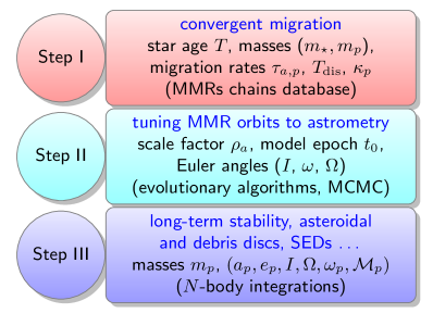
Figure 1: A graphical representation of the Migration Constrained Optimization Algorithm. Major steps and the most important parameters are listed. The diagram illustrates also a plan of this work. See the text for details.

2.1 A set of MMR captured systems

At the first step, we build a database of systems formed through migration of an appropriate number of planets. Their semi-major axes may be only roughly consistent with the observations. We consider co-planar systems, following arguments behind the planetary migration theory (e.g., Armitage, 2018, and references therein). Orbital elements such as eccentricity, nodal angle and the mean anomaly are self-consistently tuned by the migration. The planetary masses may be constrained by cooling models (Baraffe et al., 2003; Marleau & Cumming, 2014) or sampled from a preselected distribution.

We may consider any reasonable variant of the migration theory at this stage. The crucial point is that the planetary migration leads to the MMR capture, and establishes stable systems. In order to mimic the migration with the $N$-body code, we modify the astrocentric equations of motion with a force term (Papaloizou & Terquem, 2006; Beaugé et al., 2006; Moore et al., 2013)

$${\boldsymbol{f}}_{i}=-\frac{{\boldsymbol{v}}_{i}}{2\tau_{i}}-\frac{{\boldsymbol{v}}_{i}-{\boldsymbol{v}}_{c,i}}{\kappa_{i}^{-1}\tau_{i}},$$ (1)

where ${\boldsymbol{v}}_{i}$ is the astrocentric velocity of planet $i=1,2,3,\ldots,N$, ${\boldsymbol{v}}_{c,i}$ is a velocity of planet $i$ at a circular Keplerian orbit at the distance of this planet. We note that the HR 8799 planets are numbered with $i=1,2,3,\ldots$ with respect to their increasing distance from the star, or, we mark them with Roman letters, from the innermost “e” $\equiv$ “1” to the outermost “4” $\equiv$ “b” or “f” $\equiv$ “5”, following the order in which they were discovered and named (Marois et al., 2008, 2010).

The timescale of migration of planet $i$ is denoted with $\tau_{i}$, while $\kappa_{i}$ is the ratio between $\tau_{i}$ and the timescale of orbital circularization, which may be uniform for all planets in the system. Moreover, $\tau_{i}$ could depend on time, that simulates a dispersal of the disc, i.e., $\tau_{i}=\tau_{i}(t=0)\exp(t/T_{\rm dis})$, where $T_{\rm dis}$ is the characteristic time of the decay.

  

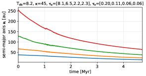
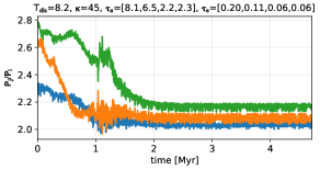
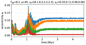
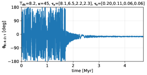
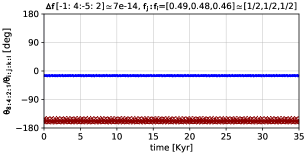
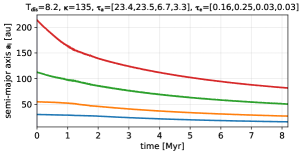
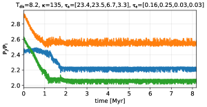
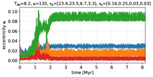
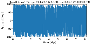
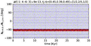
Figure 2: The migration capture of four HR 8799 planets into the generalized Laplace resonances. Panels from the top to bottom illustrate temporal evolution of the semi-major axes, orbital period ratios of subsequent pairs of planets, eccentricities, and the critical arguments (two bottom panels), respectively. The disk decay timescale $T_{\rm dis}$, as well the migration time-scales $\tau_{\rm a}$ and $\tau_{\rm e}\equiv\kappa^{-1}\tau_{a}$ in square brackets are in Myrs; $P_{j}:P_{i}$ and $f_{j}:f_{i}$ mean ratios of the astrocentric orbital periods and the proper mean motions $f_{i}$ for subsequent pairs of planets; $\Delta f[\eta_{1},\eta_{2},\eta_{3},\eta_{4}]$ is for the absolute range of the linear combination of the frequencies $f_{i}$, and is expressed in radians per the so called long day of $2\pi\,$yr${}^{-1}\simeq 58.13$ d. All panels were generated in course of the simulations. See the text for more details.

The migration experiments described below were conducted with the initial semi-major axes by three-four times as large as in the observed system, yet each one selected randomly within $50$% deviation from its nominal values for the 8e:4d:2c:1b Laplace resonance. The initial eccentricities were selected randomly, $e_{1,2,3,4}\in[0,0.16)$. The pericenter arguments $\varpi_{i}$ and the mean anomalies ${\cal M}_{i}$ were drawn from the uniform distribution in $[0^{\circ},360^{\circ}$). As for the planetary masses $m_{i}$, we choose the uniform distribution limited within $[6,{10}$] $\,\mbox{m}_{{\mbox{\scriptsize Jup}}}$ range.

In order to introduce a variability in the outcome configurations, we considered a few variants of Eq. 1, with $\kappa_{i}$ selected randomly for each planet around a mean $\kappa\in[1,300)$, or by choosing it the same for all planets. We also randomly changed the dispersal time $T_{\rm dis}\in[1,30]$ Myr, or it was infinite. We randomised individual timescales of the migration $\tau_{i}\in[1,30]$ Myr, forming a decreased sequence, in order to obtain convergent migration.

The equations of motion were integrated until a traced system did not disrupt and the hierarchy of the initial semi-major axes was preserved. We stopped the integrations when the inner semi-major axis in the migrating systems becomes $a_{1}<14.6$ au. Then we integrated the $N$-body equations of motion without dissipation for additional 32768 steps of 400 days ($\sim 1/40$ of the innermost period), in order to determine the proper mean motions for all planets. The proper mean motions are the fundamental frequencies $f_{i}$ resolved with the refined Fourier frequency analysis (Laskar, 1993; Šidlichovský & Nesvorný, 1996) of the time series $\{a_{i}(t)\exp(\mbox{i}\lambda_{i}(t))\}$, where $a_{i}(t)$ and $\lambda_{i}(t)$ are the canonical osculating semi-major axis and the mean longitude, respectively, as inferred in the Jacobi or Poincaré frame. Then we computed the linear combinations of the fundamental frequencies,

$$\Delta f({\boldsymbol{n}})\equiv\sum_{i=1}^{N}n_{i}f_{i},$$

where ${\boldsymbol{n}}\equiv[n_{1},\ldots,n_{N}]$ is a vector of integers in the $[-6,6]$ range, which yield small $|\Delta f|$. In this way, we aimed to find possible, low-order multi-body mean motion resonances (MMRs chains). Simultaneously, we examined critical angles corresponding to ${\boldsymbol{\eta}}=\mbox{arg}\min|\Delta f({\boldsymbol{n}})|$

$$\theta_{{\boldsymbol{\eta}}}(t)\equiv\sum_{i=1}^{N}\eta_{i}\lambda_{i}.$$

If $|{\boldsymbol{\eta}}|=0$, in accord with the d’Alambert rule, then the resonant configuration may be called the generalized Laplace resonance (Papaloizou, 2015), or the multiple MMR chain of the zero-th order.

Two typical examples of the resonance capture of four-planet systems are illustrated in Fig. 2. The left column is for a system trapped in the generalised Laplace resonance which exhibits librations of at least two critical angles, with amplitudes of several degrees: the “classic” Laplace resonance, which we studied in (Goździewski & Migaszewski, 2014), is distinguished through

$$\theta_{8:4:2:1}\equiv\theta_{1:-2:-1:2}=\lambda_{1}-2\lambda_{2}-\lambda_{3}+2\lambda_{4},$$

as well as another critical angle $\theta_{-1:4,-5:2}$. In this four-body MMR chain, the orbital period ratios are pairwise close to 2.

The second example in the right column of Fig. 2 shows a zero-th order four-body MMR with librations of only one critical angle $\theta_{-1,4,-6,3}$ ($\theta_{8:4:2:1}$ circulates). Moreover, the middle pair of planets exhibits the orbital period ratio close to 2:5 (see the bottom plot with $\Delta f$ in Fig. 2).

In both cases, the inner eccentricities are excited to moderate values of $\simeq 0.1$, which usually leads to good orbital fits.

Figure 3 shows the distribution of osculating astrocentric orbital periods and eccentricities attained when $a_{1}<14.6$ au. At this moment, which is the reference zero-epoch for further optimization, the migration simulation was stopped. A feature of this distribution is an over-populated regime of 2:1 MMR for subsequent pairs of planets. The 2:1 MMR appears most “easily”, in spite of significantly varied initial orbits, masses and migration parameters. The final eccentricities may be as large as 0.2, yet the most frequent values are found around 0.02–0.05.

The statistics of migrated configurations illustrated in Fig. 3 involves also a significant fraction of systems with the innermost and the outermost pairs in the 3:1 MMR. However, such systems do not fit observations since the semi-major axis of HR 8799b appears too wide, $a_{\rm b}\sim 80$ au.

An interesting result flowing from identification of the MMRs is a dominant proportion of the zero-th order MMR chains, which may be estimated as large as $\sim 90\%$ in the total sample of $\sim 1.5\times 10^{5}$ systems. It may deserve further study, which we aim to conduct in a separate work.

Similar results were obtained at early preparation of this paper, regarding five planets systems, with a hypothetical planet HR 8799f beyond the orbit of HR 8799b, and with a small mass of $\simeq 2~{}\,\mbox{m}_{{\mbox{\scriptsize Jup}}}$ below the present detection level. In this case, the initial spread of semi-major axes in migrating systems was more close ($\pm 20\%$) to the 2:1 MMRs for subsequent pairs. Regarding eccentricity, the only qualitative difference with the four-planet simulations is a longer tail in the histogram for planet b, extended for $e_{\rm b}\sim 0.15$, which is forced by the outer planet HR 8799f.

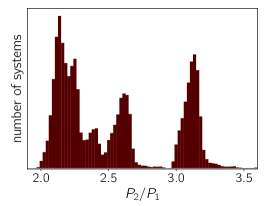
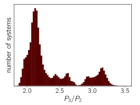
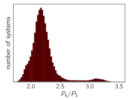
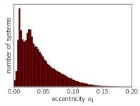
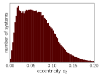
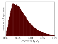
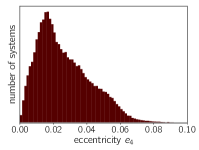
Figure 3: A graphical representation of the MCOA database that consists of $\sim 1.5\times 10^{5}$ four-planet configurations obtained through the planetary migration. The top row is for the distribution of osculating, astrocentric period ratios at the epoch zero, when inner semi-major axis $a_{\rm e}<14.6$ au. Peaks in the top row indicate low-order two-body MMRs. The bottom row is for the distribution of osculating, astrocentric eccentricities at the zero-epoch.

Here, we consider essentially the most simple model of the migration. One could apply more sophisticated theories accounting for the mass growth, or stochastic migration (Papaloizou & Terquem, 2006; Armitage, 2018). At this stage it is more important to gather a large set of orbital elements representing long-term stable systems, trapped in possibly different MMRs, rather than analysing the process in fully realistic settings.

2.2 Constraining MMR orbits with astrometric data

At the next step II, the MMR trapped systems from the MCOA database are fine-tuned to fit particular or all available observations. Only a fraction of them may reproduce the observed system. Here, we rely on the scale-free property of the $N$-body equations of motion, which allows for scaling the semi-major axes through a factor of $\rho_{a}>0$, without changing a dynamical character of the scaled system.

We find the osculating epoch $t_{0}\in[-T_{0},T_{0}]$, relative to the end-time of the migration (zero-epoch), where $T_{0}$ is typically $\sim 10^{3}$ outermost periods, since the orbits have different orbital periods and they quickly precess. We also need to fit three Euler angles $(I,\Omega,\omega)$ which rotate the orbital plane of the original system to the observer (sky) plane. The synthetic astrocentric signal is derived by propagating linearly re-scaled orbits through the numerical solution of the $N$-body equations of motion for time $t_{0}$, relative to the zero-epoch of the migration, with the initial eccentricities and orbital phases of their self-consistent, MMR-fixed values. The parameters ${\boldsymbol{p}}=(\rho_{a},t_{0},I,\Omega,\omega)$ are arguments of the merit function expressed as $\chi^{2}_{\nu}({\boldsymbol{p}})$ or the maximum likelihood function $\log{\cal L}({\boldsymbol{p}})\sim-\chi^{2}_{\nu}({\boldsymbol{p}})/2$ (Bevington & Robinson, 2003). We use the Bulirsh-Stoer-Gragg (BSG) numerical integrator to solve the equations of motion (Hairer et al., 2002). The absolute and relative local error limits are set to $\sim 10^{-15}$.

We underline that the astrocentric model of the observations is based on the self-consistent, canonical $N$-body dynamics, unlike Keplerian, geometric parametrization used frequently in the literature. The $N$-body model is more CPU-demanding, but it explicitly accounts for the planetary masses and the mutual gravitational interactions between the planets. We demonstrate its importance, when discussing the results (Sect. 3).

The optimization is performed for a number of MMR systems with the help of evolutionary algorithms (Price et al., 2005; Izzo et al., 2012; Charbonneau, 1995). Furthermore, the Bayesian inference and MCMC sampling makes it possible to introduce prior information on the system parameters, in order to estimate their uncertainties and correlations. We choose models yielding reasonably small $\chi^{2}_{\nu}$ as the best-fitting solutions.

What separates the planetary migration (Step I) from the orbital optimization (Step II) is the scale-free property of the $N$-body Newtonian dynamics. In the barycenter frame they read as follows

$$\ddot{{\boldsymbol{r}}}_{i}=k^{2}\sum_{j}m_{j}\frac{{\boldsymbol{r}}_{ji}}{|{{\boldsymbol{r}}}_{ji}|^{3}},\quad i\neq j=0,\ldots,N,$$ (2)

where ${{\boldsymbol{r}}_{ji}}\equiv{{\boldsymbol{r}}}_{j}-{{\boldsymbol{r}}}_{i}$ is the relative radius vector from a body $i$ to a body $j$, where $i,j=0$ denotes the star, $m_{j}$ are for the masses ($m_{0}\equiv m_{\star}$), and $k^{2}$ is the gravitational constant. The scaling invariance of the particular Ordinary Differential Equations (ODEs), here Eqs. 2, means that if a particular ${\boldsymbol{r}}_{i}(t)$ is the solution to these equations, then $\rho_{a}^{-2/3}{\boldsymbol{r}}_{i}(\rho_{a}t)$ with some fixed and constant scaling factor $\rho_{a}>0$ is also the solution. Therefore the orbital radii, or orbital arcs at prescribed time intervals, may be scaled by the same factor, yet with an appropriate time change. Such a geometrically re-scaled copy of the orbits exhibits the same dynamical character as the original system.

The $N$-body ODEs scaling invariance is illustrated in Fig. 4. By following a migrating planetary configuration, we usually end up with too compact (the left column) or too wide (the right column) orbits, with respect to the observations. In fact, these configurations are re-scaled copies, by a factor of 0.8 and 1.33, respectively, of the directly simulated system in the middle column. Apparently, it fits relatively well to the observations. This resonant configuration has been obtained through a fast migration during only 1.8 Myr. In spite of a substantial scaling, the dynamical character of all configurations is preserved for at least 100 Myr: the critical angles of the zero-th order generalized Laplace resonance (Papaloizou, 2015) oscillate around the same center, as well as the eccentricities vary within the same limits (the middle- and bottom panels in Fig. 4).

We note that the reference configuration is weakly chaotic in the sense of a small mLCE. However, in this Lagrange-stable configuration, all orbits remain bounded for a very long time. The system remains stable since it is resonant, actually in an unusual way – one of the critical arguments librates around the same libration center, while the second one “switches” between two centers. This example is selected intentionally, to show that even weakly chaotic configurations may be scaled without loosing any of the geometric features, like the critical angles or eccentricity evolution.

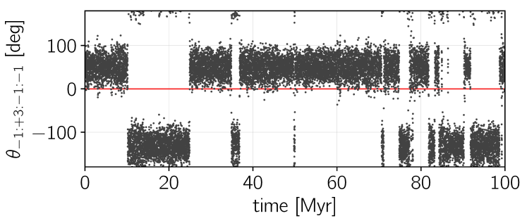
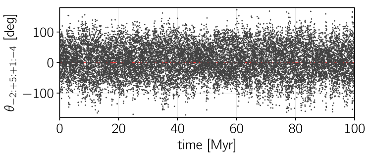
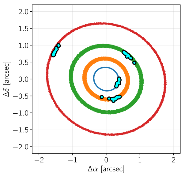
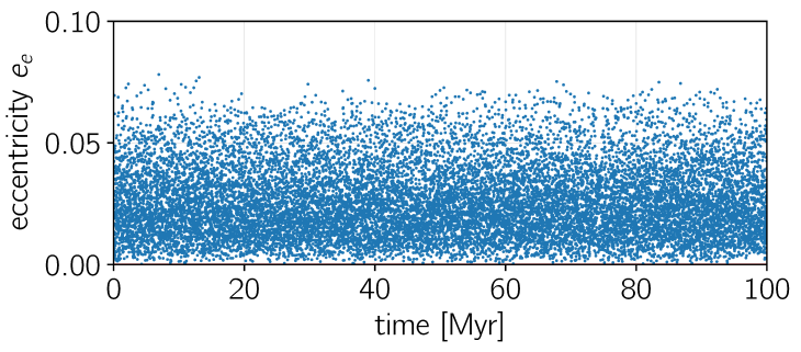
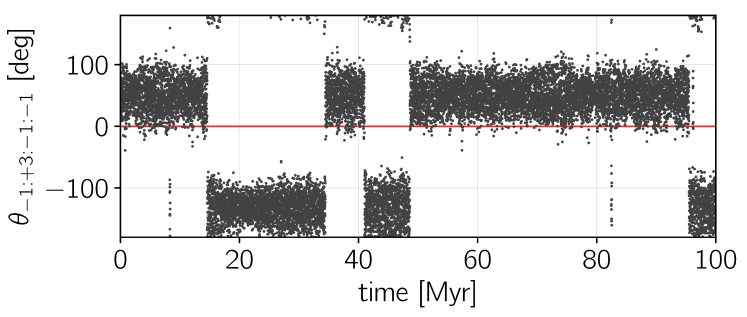
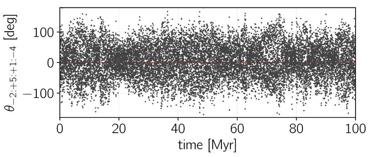
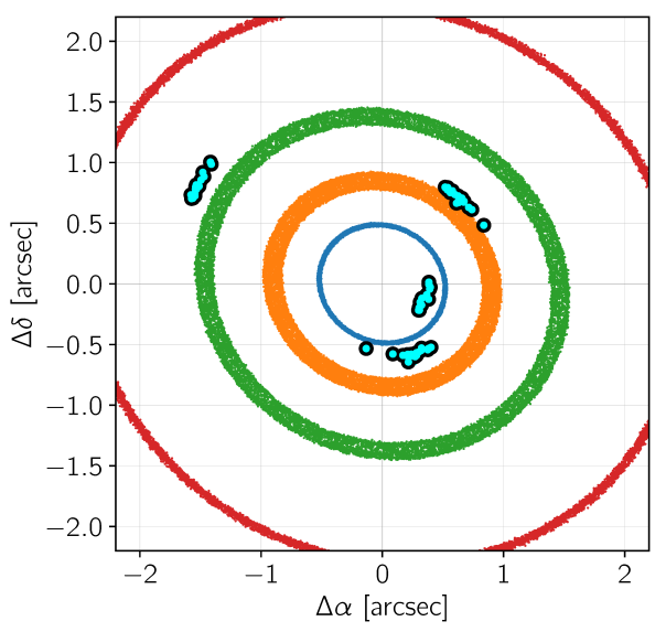
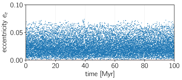
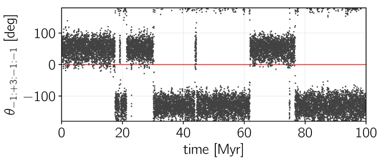
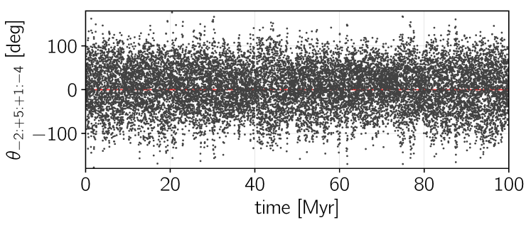
Figure 4: Illustration of scale-free dynamics at the second step of MCOA. Initial semi-major axes in a resonant configuration of four planets shown in the middle column are linearly scaled by a factor of $0.8$ (the left column), and by a factor of $1.33$ (the right column), respectively. We selected two critical arguments of the generalized Laplace resonance, $\theta=\lambda_{1}-3\lambda_{2}+\lambda_{3}+\lambda_{4}$ and $\theta=2\lambda_{1}-5\lambda_{2}-\lambda_{3}+4\lambda_{4}$, respectively (two middle rows) which librate with similar amplitudes (two bottom rows). The innermost eccentricity (the second row from top), shown as an example, varies within similar limits.

The scale-free dynamics property releases us from an uncertainty of the star distance. The present determination of the parallax $\pi=24.22\pm 0.09$ mas ($\sim 41.3$ pc) in the GAIA Data Release 2 catalogue (Gaia Collaboration et al., 2018) places the system almost 2 pc farther than assumed in the literature to date, $d=39.4$ pc (van Leeuwen & Fantino, 2005). The relatively significant correction of the parallax has essentially no implication on the orbital models, besides the planetary masses may be larger due to a correction for the absolute luminosity.

3 The best-fitting orbital model

We searched for the best-fitting solutions to the astrometric measurements in (Konopacky et al., 2016) with the approach described above. Homogeneous observations of the HR 8799 system in (Konopacky et al., 2016) are obtained between 2007 and 2014 with NIRC2 on the Keck II telescope and with the same reduction pipeline. The data are corrected for systematic biases present in observations in the discovery papers (Marois et al., 2008, 2010). Keplerian (kinematic) solutions in (Konopacky et al., 2016) favour co-planar, low eccentric orbits, as well as agree to within $1\sigma$ with the 8e:4d:2c:1b resonance model, hence our assumptions are supported by their independent analysis.

We aim to verify whether the MCOA model of these observations, which are a subset of data available to date and gathered in (Wertz et al., 2017, their Appendix), may be extrapolated and fit all measurements made by different authors with other instruments. We also found a significant deviation of the synthetic model orbit IVa in (Goździewski & Migaszewski, 2014) for the outermost planet, which systematically precedes the latest observations in (Pueyo et al., 2015) and (Maire et al., 2015). The new analysis could improve the previous model.

Among the found solutions, we selected the best-fitting configuration yielding $\chi^{2}_{\nu}~{}\simeq 0.87$. Its osculating elements at epoch $t_{0}=2004.532{}$ of the first observation in (Konopacky et al., 2016), as determined from the primary fit parameters ${\boldsymbol{p}}$, are displayed in Tab. 1 (model IV_K). We found tens of geometrically similar configurations within $\chi^{2}_{\nu}\simeq 1$, therefore we focus on this particular, basis configuration. This model, representing the 8e:4d:2c:1b MMR chain, is similar to the best-fitting solution IVa in (Goździewski & Migaszewski, 2014). Yet we note a smaller value of the initial semi-major axis $a_{4}\simeq 67$ au. We examined this difference closely. As expected, the new solution improves the astrometric model by providing a better match to the first and the last observations at epochs of 1998.83 and 2014.93 in the whole data set, respectively. Indeed, it removes the systematic trend and the “too fast” orbital motion of planet b predicted by our earlier model IVa.

Table 1: Osculating elements of the best-fitting four- and five-planet solutions. For model IVa reproduced from (Goździewski & Migaszewski, 2014), the osculating epoch is $1998.83$, and the stellar mass $m_{\star}=1.56\,\mbox{M}_{\odot}$. Model IV_K found in this work is determined at the osculating epoch of 2004.532 and for the star mass of $m_{\star}=1.52\,\mbox{M}_{\odot}$. Co-planar solutions postscripted with “A”, “B”, “C”, “D” and “E” extend model IV_K with a fifth hypothetical planet in a stable orbit. Model IV_MCMC is a non-coplanar four-planet stable solution with small $\chi^{2}_{\nu}\simeq 1$ found with the MCMC sampling around model IV_K. These models are solutions to the measurements in (Konopacky et al., 2016). Model V_A is a preliminary fit to all observations collected in (Wertz et al., 2017), and found with the MCOA for a five-planet system. Uncertainties for parameters in models IV_K and IV_MCMC are determined as ranges of $\langle Y\rangle$-stable samples yielding $\chi^{2}_{\nu}<1.6$ around their median values. Formal errors, determined as the 16-th and 86-th percentile of the samples are by 2–3 times smaller. For a reference, parameter values for fits IV_K and IV_A with five digits after decimal point are provided, as literally used in our experiments. Parameter $\nu=N_{(\alpha,\delta)}-\dim{{\boldsymbol{p}}}$ is for the degrees of freedom, where $N_{(\alpha,\delta)}$ denotes the number of $(\alpha,\delta)$ measurements, and $\dim{{\boldsymbol{p}}}$ is the number of free parameters.

	$m\,[\,\mbox{m}_{{\mbox{\scriptsize Jup}}}]$	$a\,$[au]	$e$	$I\,$[deg]	$\Omega\,$[deg]	$\varpi\,$[deg]	$\mathcal{M}\,$[deg]
Model IVa at epoch of $1998.83$, $m_{\star}=1.56\,\mbox{M}_{\odot}$ (Fig. 7, top row)
HR 8799e	$9\pm 2$	$15.4\pm 0.2$	$0.13\pm 0.03$			$176\pm 6$	$326\pm 5$
HR 8799d	$9\pm 3$	$25.4\pm 0.3$	$0.12\pm 0.02$	$25\pm 3$	$64\pm 3$	$91\pm 3$	$58\pm 3$
HR 8799c	$9\pm 3$	$39.4\pm 0.3$	$0.05\pm 0.02$			$151\pm 6$	$148\pm 6$
HR 8799b	$7\pm 2$	$69.1\pm 0.2$	$0.020\pm 0.003$			$95\pm 10$	$321\pm 10$
Model IVK at epoch of 2004.532, $m_{\star}=1.52\,\mbox{M}_{\odot}$, $\chi^{2}_{\nu}=0.87$, $\nu=97$, $\dim{{\boldsymbol{p}}}=5$ (Figs. 8–11)
HR 8799e	$9.4\pm 0.5$	$15.45\pm 0.25$	$0.127\pm 0.011$			$107.5\pm 1.5$	${13.7}\pm 1.5$
	9.426	15.45001	0.12696			107.54637	13.67259
HR 8799d	$8.2\pm 0.8$	$25.36\pm 0.30$	$0.095\pm 0.006$			$26.9\pm 2.5$	$79.4\pm 3.0$
	8.185	25.35505	0.09540			26.94575	79.41486
HR 8799c	$6.9\pm 0.5$	$39.78\pm 0.40$	$0.048\pm 0.005$	$25\pm 2$	$64\pm 5$	${105.8}\pm 2.0$	${137.2}\pm 5.0$
	6.857	39.77699	0.04829	25.289	64.414	105.79908	137.18943
HR 8799b	${6.7}\pm 0.5$	$67.01\pm 0.35$	$0.023\pm 0.003$			${120.1}\pm 3.0$	${235.7}\pm 5.0$
	6.680	67.00881	0.02297			120.07543	235.66545
HR 8799fA	1.660	115.25600	0.02222			174.59807	54.13554
HR 8799fB	0.660	116.43105	0.02222			174.59807	54.13554
HR 8799fC	1.000	134.16610	0.02218	25.289	64.414	11.33805	327.42380
HR 8799fD	0.330	133.86900	0.02218			11.33805	327.42380
HR 8799fE	0.100	137.76200	0.02218			11.33805	327.42380
Model IVMCMC at epoch of 2004.532, $m_{\star}=1.52\,\mbox{M}_{\odot}$, $\chi^{2}_{\nu}=0.98$, $\nu=74$, $\dim{{\boldsymbol{p}}}=28$    (Fig. 6)
HR 8799e	$9.5\pm 0.5$	$15.48\pm 0.25$	$0.123\pm 0.011$	$26\pm 2$	$64\pm 5$	$110.2\pm 1.5$	$12.5\pm 1.5$
	9.489	15.48223	0.12278	26.138	63.612	110.23990	12.49904
HR 8799d	$7.5\pm 0.8$	$25.35\pm 0.30$	${0.097}\pm 0.006$	$29\pm 2$	$56\pm 5$	$33.1\pm 2.5$	$80.8\pm 3.0$
	7.490	25.35133	0.09669	29.096	56.160	33.05848	80.78110
HR 8799c	$7.1\pm 0.5$	$39.95\pm 0.40$	$0.046\pm 0.005$	$25\pm 2$	$63\pm 5$	$104.8\pm 2.0$	$140.0\pm 5.0$
	7.082	39.94936	0.04629	25.318	62.732	104.77760	139.98150
HR 8799b	$6.8\pm 0.5$	$67.11\pm 0.35$	$0.024\pm 0.003$	$31\pm 2$	$60\pm 5$	$118.5\pm 3.0$	$242.9\pm 4.5$
	6.753	67.11155	0.02358	30.517	59.595	118.49210	242.91630
Model VA at epoch of 1998.83, $m_{\star}=1.52\,\mbox{M}_{\odot}$, $\chi^{2}_{\nu}=2.71$, $\nu=229$, $\dim{{\boldsymbol{p}}}=5$ (Fig. 7, bottom row)
HR 8799e	$9.450$	15.45863	0.09789			115.18157	330.89613
HR 8799d	$6.851$	25.59693	0.09300			29.67592	62.45914
HR 8799c	$7.121$	39.78074	0.05227	26.103	60.210	101.42421	136.56084
HR 8799b	$8.847$	70.24633	0.05055			52.58777	306.83016
HR 8799f	$2.500$	111.48326	0.01205			140.41787	65.69502

3.1 Measuring stability of orbital solutions

In order to reveal the global dynamical structure of the system, we use the fast indicator technique, besides the direct integration of the equations of motion. The idea behind this approach relies in determining the character of motion (chaotic or regular) on relatively short orbital arcs. A configuration classified as the fast indicator-stable for relatively short motion time of $\simeq 10^{4}$ outer periods may be extrapolated for 10-100 longer Lagrange stability time (called also the event time, $T_{\rm E}$), implying non-crossing, non-colliding and bounded orbits. Usually, the fast indicators are related either to the maximal Lyapunov Characteristic Exponent (mLCE, Cincotta & Simó, 2000; Goździewski et al., 2008) or to a diffusion of the fundamental frequencies (Laskar, 1993).

As the fast indicator, essentially equivalent to the mLCE, we use the Mean Exponential Growth factor of Nearby Orbits (MEGNO, or $\langle Y\rangle$ from hereafter) developed by Cincotta & Simó (2000); Cincotta et al. (2003). It is implemented in our Message Passing Interface (MPI) parallelized code $\mu$Farm. The required system of the equations of motion and their variation equations may be integrated with the Bulirsh-Stoer-Gragg (BSG) scheme (Hairer et al., 2002). We also used the symplectic algorithm (Goździewski et al., 2008), which is much more CPU efficient, but it might be non-reliable in strongly chaotic zones where collisional events are possible. We decided to use the BSG scheme for final experiments, to avoid such numerical and artificial biases.

For brevity, orbital configurations are called $\langle Y\rangle$-stable if $\left|\langle Y\rangle-2\right|<\epsilon$, where $\epsilon\simeq 0.05$, for a particular number of characteristic periods, counted in $10^{4}$ outermost planet orbits. The MEGNO integrations were stopped if $\left|\langle Y\rangle-2\right|>5$, and we consider such configurations as unstable ($\langle Y\rangle$-unstable). As we found in previous papers, $\langle Y\rangle$-stable models are equivalent to Lagrange-stable solutions for one-two orders of magnitude longer intervals of time.

More details on these MEGNO calibration to determine the Lagrange stability, regarding the HR 8799 system, and also low-mass planet systems were discussed in our earlier papers (Goździewski et al., 2008; Goździewski & Migaszewski, 2014) as well as in a new work (Panichi et al., 2017). We also note that MEGNO has been recently used as a reference tool by Hadden & Lithwick (2018), who developed a new, quasi-analytic stability criterion for eccentric two-planet systems.

3.2 The MCMC experiments setup

We conducted followup MCMC experiments, aiming to determine the orbital parameter uncertainties for stable solutions found with MCOA, and to demonstrate the degree of instability of the four-planet system. For that purpose we performed single-temperature MCMC sampling with the emcee package (Foreman-Mackey et al., 2013). Recalling our results in (Goździewski & Migaszewski, 2014), the orbital elements in stable four-planet models may be only varied within tiny ranges. Here, we release the co-planarity constraint and we search for stable solutions around the best-fitting model IV_K. The Bayesian inference makes it possible to introduce prior information, like indirect observational constraints. For instance, the debris disks geometry determined independently of the imaging astrometry are reported almost coplanar with the planetary orbits, and seen at the position angle around of $50^{\circ}$–$60^{\circ}$ (Matthews et al., 2014; Booth et al., 2016). Therefore the debris disk models could impose additional, indirect constraints on the inclination $I$ and nodal angle $\Omega$ of the system.

With the MCMC sampling of the parameter space, stable planetary configurations might be detected, perhaps relatively distant from the model IV_K in Tab. 1. Therefore, in the search for stable solutions, we conducted the MCMC sampling with up to 2048 emcee walkers initiated in a small hyper-cube in the orbital parameter space centered at the best-fitting model, for 128,000 to 256,000 iterations each, mostly limited by CPU-demanding stability checks made with the MEGNO indicator. We evaluated $\chi^{2}_{\nu}$ and the likelihood function $\log{\cal L}\sim-\chi^{2}_{\nu}/2$ required to compute the posterior distribution. In this experiment, masses of the planets and all orbital elements are considered as free parameters of the astrometric model.

In order to narrow the parameter space, and to reduce possible degeneracies, we imposed Gaussian priors ${\cal N}(\mu,\sigma_{\mu})$ with the mean $\mu$ equal to the best-fitting values in Tab. 1. As for the variances $\sigma_{\mu}$, we choose: for the masses, $\sigma_{m}=3\,\,\mbox{m}_{{\mbox{\scriptsize Jup}}}$; for the semi-major axes, $\sigma_{a}=5$ au; for the Poincaré elements $x_{i}=e_{i}\cos\omega_{i}$, and $y_{i}=e_{i}\sin\omega_{i}$, $\mu_{x,y}=0$ and $\sigma_{x,y}=0.3$; for the inclinations and the nodal longitudes, $\sigma_{I}=30^{\circ}$ and $\sigma_{\Omega}=60^{\circ}$, respectively. The priors have been set as improper (uniform) for the osculating mean anomalies at the initial epoch, ${\cal M}_{i}\in[0^{\circ},360^{\circ})$, $i=1,\ldots,4$.

During the MCMC sampling with the Gaussian priors, we also evaluated the MEGNO of all solutions with $\chi^{2}_{\nu}<2.6$, to determine limits of stability zone around the best-fitting stable solution. The $\langle Y\rangle$ integration time was set to $\simeq 7,000$ outermost periods, hence permitting for marginally Lagrange-stable models. In accord with our earlier experiments (Goździewski & Migaszewski, 2014), the $\langle Y\rangle$ integration interval should be safely longer than $10^{4}$ characteristic periods, in order to determine long-term Lagrange-stable configurations for at least 160 Myr. The $\langle Y\rangle$-stable solutions for $7,000$ outermost orbits should provide ten times longer Lagrange stability time (at least $\simeq 30$ Myr).

For a reference, we also performed the MCMC sampling with all priors uniform, and determined in wide parameter ranges, spanning 24 $\,\mbox{m}_{{\mbox{\scriptsize Jup}}}$ for masses $m_{i}$, and 30 au for semi-major axes $a_{i}$ around their best-fitting values IV_K in Table 1, as well as $x_{i},y_{i}\in[0,0.67]$ for the Poincaré elements, $I_{i}\in[0^{\circ},90^{\circ}]$, $\Omega_{i}\in[0^{\circ},180^{\circ}]$, and ${\cal M}_{i}\in[0^{\circ},360^{\circ}]$ ($i=1,\ldots,4$).

We tried to estimate the auto-correlation time $\tau_{\rm emcee}$ through sampling experiments without stability checks, in order to reduce the CPU overhead. We increased the chain length up to $512,000$. We used a method of Sokal (1996), as proposed by (Foreman-Mackey et al., 2013) in the recent version of the emcee sampler. We found that $\tau_{\rm emcee}$ is typically very long and varies between $\sim 40,000$ and $\sim 120,000$ for different elements and priors. The second parameter expressing the sampling “health”, the acceptance rate, was typically well below 0.2, unless the emcee scaling parameter $a_{\rm emcee}$ was set to low values of $\sim 1.2$. Similarly difficult and ill-conditioned Monte-Carlo and MCMC sampling experiments are reported by Konopacky et al. (2016) and Wertz et al. (2017), regarding kinematic (Keplerian) models.

We found a particularly strange discrepancy of the distribution of the node arguments $\Omega_{i}$. As reported in Konopacky et al. (2016), two $\Omega_{i}$ peaks wide for up to a few tens degrees are centered around roughly $\sim 60^{\circ}$ and $\sim 130^{\circ}$–$150^{\circ}$, respectively, for all planets but HR 8799d with one, much wider dominant peak around $\Omega_{\rm d}\sim 100^{\circ}$. The first mode around $\sim 60^{\circ}$ is consistent with the outer debris disk orientation (Matthews et al., 2014; Booth et al., 2016). However, it is missing at all among single-mode posteriors of $\Omega_{\rm c}$ and $\Omega_{\rm e}$ derived by Wertz et al. (2017). We note here that our $N$-body MCMC experiments made with fixed masses in the best-fitting solution IV_K, that could mimic the Keplerian model, yet with Gaussian priors on the eccentricity, reveal a two-modal posterior only in $\Omega_{\rm c}$, while all remaining peaks of $\Omega_{\rm b,d,e}$ are found between $50^{\circ}$ and $60^{\circ}$. This most strong two-modal distribution of $\Omega_{\rm c}$ divided with a shallow posterior valley might explain a low acceptance rate in our experiments. Also a dynamical sense of the second mode of $\Omega_{i}\simeq 130^{\circ}$, implying mutually inclined orbits, remains uncertain.

3.3 The MCMC experiments and the best-fitting model

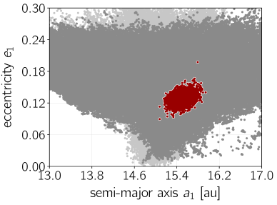
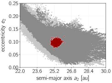
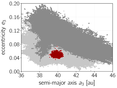
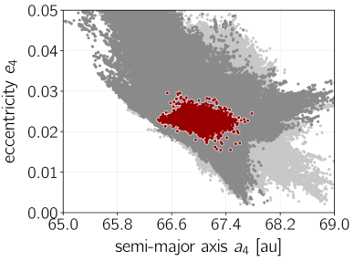
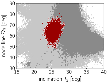
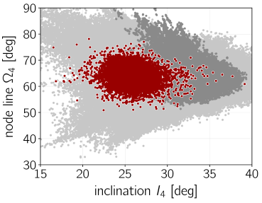
Figure 5: The results of MCMC experiments as 2-dim $\chi^{2}_{\nu}$ projections of samples onto selected parameter planes. Light-gray and dark-grey filled circles mark solutions derived with uniform priors, with $\chi^{2}_{\nu}<1.6$ and $\chi^{2}_{\nu}<0.74$, respectively. Dark-red filled circles for $\langle Y\rangle$-stable models with $\chi^{2}_{\nu}<2.6$. See Fig. 6 for the sky-plane representation of configurations selected from the illustrated samples.

Our results derived in two example MCMC experiments are illustrated in Fig. 5, as 2-dim $\chi^{2}_{\nu}$ distributions for selected parameters. The light-grey filled circles represent solutions with $\chi^{2}_{\nu}<1.6$ and darker filled circles are for samples with $\chi^{2}_{\nu}<0.74$, derived with uniform priors. We note that the lowest $\chi^{2}_{\nu}\simeq 0.60$. The dark-red filled circles mark solutions $\langle Y\rangle$-stable for $\sim 7,000$ outer periods when Gaussian priors are set only for masses and semi-major axes. The number of illustrated samples is $\sim 2\times 10^{6}$.

Clearly, even for the very limited $\chi^{2}_{\nu}<0.74$ range, the model parameters are practically unbounded. They vary in wide limits both for the uniform and Gaussian priors. Also the 1-dim posterior distributions (not shown) imply that the $N$-body astrometric model is unconstrained, similarly to the Keplerian models in (Konopacky et al., 2016) and (Wertz et al., 2017). Stable solutions are found only relatively close to the initial resonant configuration, and the overall shape of stable, compact zones agrees with the results derived with constrained genetic algorithm (see, Goździewski & Migaszewski, 2014, for details). Here, however, the search for stable non-coplanar solutions has been performed with an independent method.

We performed the same experiment for different choices of the Gaussian priors (the mean values and their $\sigma_{\mu}$) for masses and orbital elements. All these attempts to find stable configurations resulted in outputs qualitatively similar to those demonstrated in Fig. 5. We estimate that the total number of tested samples with $\chi^{2}_{\nu}<2.6$ has reached $10^{9}$ in more than 20 MCMC experiments performed on 256 CPU cores each. We did not find any $\langle Y\rangle$-stable model beyond a close neighborhood of the best-fitting, stable resonant model IV_K. Therefore finding a stable configuration by chance, or without imposing tight or a’priopri constraints on the model parameters, would be extremely difficult.

Finally, the results of the MCMC sampling experiments shown in Fig. 5 are further illustrated in Fig. 6. We selected 20 stable solutions with $\chi^{2}_{\nu}<1.04$, and 500 other (unstable) models with low $\chi^{2}_{\nu}<0.74$ from the MCMC-derived posterior samples. Their orbital arcs, marked with red and grey curves, respectively, are over-plotted on the astrometric data in (Konopacky et al., 2016) as blue, filled circles, and all other measurements in the literature collected in (Wertz et al., 2017), with yellow diamonds. In spite of the tight restriction, $\chi^{2}_{\nu}<0.74$, the grey curves span a wide region of the sky. Moreover, stable models to a subset of data in (Konopacky et al., 2016) extrapolate very well to the full data set. We may note the proper timing of the synthetic orbits both with the most recent, as well as the earliest measurements (the top-middle, the top-right and the bottom-left panels in Fig. 6).

An interesting conclusion regards the top-middle panel for planet HR 8799d. Low $\chi^{2}_{\nu}<0.74$ solutions (dark curves) widely spread around the Hubble Space Telescope (HST) observation at epoch 1998.98 in (Lafrenière et al., 2009). However, stable, resonant models pass in the middle of these solution orbits, closely to the HST measurement made a few years before. It might be a lucky coincidence, but we recall that stable solutions are extrapolated back from the model epoch of 2004.532, and the HST measurement was not included in the optimization.

One more feature of stable solutions is illustrated in the right-bottom panel of Fig. 6, showing model orbits for the two inner planets. In this panel, each of the orbits are computed for their osculating period. Surprisingly, orbital arcs of stable solutions for planet HR 8799d do not close. It means that the gravitational interactions may be detected even within the narrow observational window. It is also a warning that kinematic models which do not account for the mutual planetary interactions may be soon non-adequate in a longer time-basis.

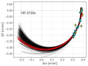
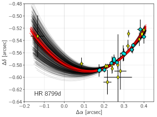
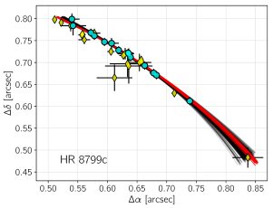
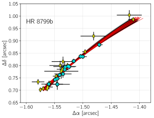
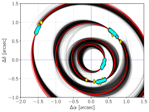
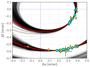
Figure 6: The best-fitting solution to the four-planet model illustrated at the sky-plane. The $y$-axis corresponds to N, and the $x$-axis corresponds to E direction, respectively (note that the numerical values of $\Delta\alpha$ are sign-opposite to regarding the formal left-hand direction of the right ascension $\alpha$). Light-blue (white-gray) filled circles are for measurements in (Konopacky et al., 2016), and dark-blue (dark-grey) filled circles are for measurements in other papers, as collected in (Wertz et al., 2017). Red curves mark several stable solutions with $\chi^{2}_{\nu}\simeq 1$ from the MCMC sampling. Grey curves are for orbital arcs derived from unstable models within $\chi^{2}_{\nu}<0.74$, marginally worse from $\chi^{2}_{\nu}\simeq 0.6$ for the mathematically best-fitting $N$-body solutions. All model orbits have been derived for measurements in (Konopacky et al., 2016), and then extended between the epochs of 1998.83 and 2014.93 in the full data set in (Wertz et al., 2017). The osculating epoch is 2004.532, i.e., the first epoch in (Konopacky et al., 2016).

In order to summarise, we consider the results of our MCMC experiments mostly as an attempt of determining the range of stable islands, rather than a rigorous optimisation and statistical inference presented in (Pueyo et al., 2015; Konopacky et al., 2016; Wertz et al., 2017). Moreover, since stability zones are extremely tiny with respect to wide posteriors, the results of statistically reliable MCMC sampling made with the kinematic orbital model (without stability checks) might bring only limited information on stable solutions.

4 The $\langle Y\rangle$-model of debris disks

Having the long-term stable configurations of the system, we may simulate debris disks in a framework of the restricted and non-restricted problems. In the first version, mass-less particles (asteroids) are influenced by the gravitational tug of the planets (primaries), and we assume that the asteroids do not attract the planets nor mutually interact. In the second, non-restricted case, hypothetical massive bodies may be added to the system of observed planets. Such bodies may be detected indirectly through resolving the global architecture of the observed system. For instance, a signature of the fifth planet beyond HR 8799b may be the radius of the inner edge of the outer debris disk (Booth et al., 2016). Also Wilner et al. (2018) constrained a mass of the outer planet HR 8799b to $\simeq 6\,\mbox{m}_{{\mbox{\scriptsize Jup}}}$ through modeling the inner edge with ALMA and VLA observations. Based on the ALMA observations alone, Read et al. (2018) deduced a mass of an additional planet HR 8799f beyond the orbit of planet b.

We conducted extensive Monte Carlo simulations of the debris disks in both frameworks. The initial semi-major axis, as well as eccentricity and orbital phases are drawn randomly within prescribed ranges. These elements extend the initial condition for the observed planets (primaries), and the resulting orbits are integrated. We then analyze a large volume of the initial conditions with two numerical methods.

For simulating the debris disk as the restricted problem, we use the direct $N$-body integrations with the hybrid scheme in the Mercury 6.3 package (Chambers, 1999), corrected by de Souza Torres & Anderson (2008). This approach is common in the literature (e.g., Contro et al., 2016; Read et al., 2018). We fixed the step-size of 64 days for the mixed variables leapfrog (MVS) and the local accuracy $\epsilon=10^{-13}$ in the BSG algorithm, providing the relative energy error as small as $10^{-9}$.

The second numerical model makes use of the fast indicator idea and relies in determining stability of the test orbits through their $\langle Y\rangle$-signature, following arguments in Sect. 3.1. We call the approach as the $\langle Y\rangle$-model from hereafter.

The results of simulations, which are osculating orbital elements of stable systems, are projected onto the Cartesian coordinates $(x,y)$-plane, and also are shown in the semi-major axis–eccentricity $(a,e)$-plane. It helps to reveal and identify resonant structures in the phase space.

We conducted two CPU-intensive tests, on up to 256 CPU cores, to validate the $\langle Y\rangle$-model for debris disk through the direct numerical integrations. Computations are carried out for fixed masses of the bodies moving in the same plane.

4.1 The restricted four-planet system

In the first test, including four planets, we conducted a number of Mercury 6.3 runs with up to 4096 mass-less particles each. Our primary goal of this, and of further experiments, is to reconstruct the inner edge of the outer disk, hence we limit the semi-major axes to smaller range than predicted for the whole radius as large as $\sim 450$ au. Beyond the inner region of the disk, filled with strong MMRs, the population of asteroids might be determined with some quasi-analytic distribution (Booth et al., 2016; Read et al., 2018).

In order to compare the results with findings in earlier papers, the initial conditions of the planets in this experiment are the same as in the best-fitting model IVa in (Goździewski & Migaszewski, 2014), also Tab. 1. We integrated the orbits of primaries and mass-less particles for 34 Myr, which may be considered as the low limit of the system age. The simulation has been restricted to the inner part of the disk, i.e., the initial semi-major axes $a_{0}(t=0)\in[60,150]$ au. We sampled eccentricities $e_{0}(t=0)\in[0,0.33]$, as well as orbital phases randomly, with $\varpi_{0},{\cal M}_{0}\in[0^{\circ},360^{\circ})$.

The total number of particles traced with the direct $N$-body integration was $\simeq 6\times 10^{5}$. Figure 7 shows two snapshots of the simulation at $t=7$ Myr (the top-left panel), and at the end of the integration interval, $t=34$ Myr (the top-right panel). They represent instant coordinates of mass-less asteroids which have not been ejected beyond 1000 au. The final snapshot encompasses $3.7\times 10^{5}$ objects surviving the integration.

The MEGNO test is illustrated in the top-middle panel of Fig. 7. Almost $10^{6}$ particles with $\langle Y\rangle$ are marked at the integration time of $7$ Myr, which corresponds to $\sim$14,000 orbital periods of the outermost planet and roughly 8,000 revolutions at $\simeq 100$ au. Particles marked as $\langle Y\rangle$-stable for that interval should persist for more than 10 times longer interval in Lagrange-stable orbits, roughly $60$–$70$ Myr. Indeed, the inner border of the debris disk derived with the direct Mercury 6.3 integration looks very similar to the non-circular oval shape revealed by the $\langle Y\rangle$-model.

A different density of particles in the two snapshots may be explained by a sampling strategy. In regions, where the test orbits are strongly chaotic, like just beyond the orbit of HR 8799b, the motion is $\langle Y\rangle$-unstable during short intervals $\simeq 0.1$ Myr, and the $\langle Y\rangle$ integration may be stopped as soon as $\langle Y\rangle>5$, safely larger than $\langle Y\rangle\simeq 2$ for stable systems. That made it possible to examine huge sets of $\sim 10^{8}$ initial conditions, orders of magnitude larger than they could be sampled with the direct $N$-body integrations. Such strongly chaotic regions are explored in a CPU-efficient way, and we argue that the inner, complex edge may be revealed more detailed with the $\langle Y\rangle$-model.

We also note similarly extended Lagrange islands $L_{4}$, $L_{5}$ of stable particles, indicating a sensitivity of the $\langle Y\rangle$ indicator for unstable solutions.

The $\langle Y\rangle$-model plot at the $(x,y)$-plane of Cartesian coordinates may be understood as a snapshot of all possible, stable (quasi-periodic, regular) orbits of the probe masses with various orbital phases and eccentricity for the same values of the semi-major axis. These orbits might be populated in a real system, but not necessarily they are. The actual population of asteroids may depend on the prior planetary system history, its migration, as well as locally variable density of asteroids.

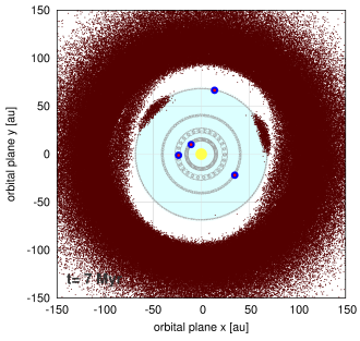
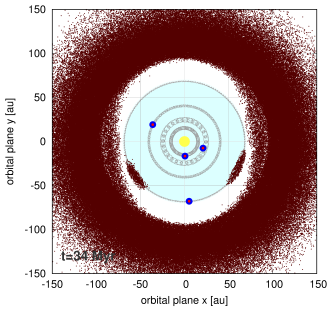
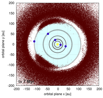
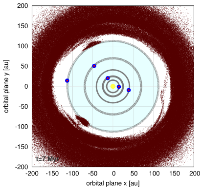
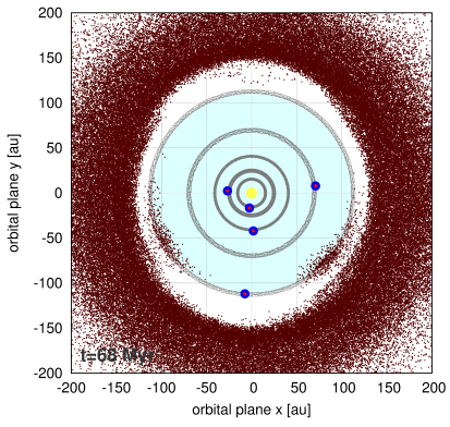
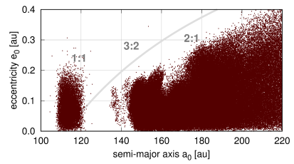
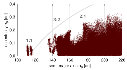
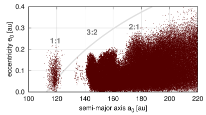
Figure 7: Top row: the outer debris disk of the four-planet HR 8799 system, in accord with model IVa in (Goździewski & Migaszewski, 2014). The left-hand and the right-hand panels show snapshots of astrocentric coordinates $(x,y)$ of mass-less asteroids at the orbital plane, at times $\simeq 7$ Myr and $\simeq 34$ Myr, respectively, derived with the direct $N$-body integrations conducted with the Mercury 6.3 package (the hybrid scheme). Filled circles are for positions of the planets, and light-grey curves are orbital arcs sampled for the times-span $\simeq 34$ Myr. The final snapshot involves $370,000$ mass-less particles which survived the integration. The middle panel shows astrocentric coordinates $(x,y)$ of $\simeq 10^{6}$ test particles with masses $10^{-15}~{}\,\mbox{m}_{{\mbox{\scriptsize Jup}}}$ in $\langle Y\rangle$-stable orbits. Middle row: the outer debris disk of the five-planet HR 8799 model V_A (Tab. 1). The left-hand and the right-hand panels show snapshots of astrocentric coordinates $(x,y)$ of mass-less asteroids at the orbital plane, at the motion times $\simeq 7$ Myr and $\simeq 68$ Myr, respectively. Planet orbits are sampled and marked with grey dots for $\simeq 68$ Myr. The final snapshot involves $125,000$ mass-less particles which survived the integration. The middle panel is for astrocentric coordinates $(x,y)$ of $\simeq 1.5\times 10^{6}$ test particles with masses $10^{-15}~{}\,\mbox{m}_{{\mbox{\scriptsize Jup}}}$ in $\langle Y\rangle$-stable orbits. Integrations done with the $\mu$Farm package. Bottom row: Osculating, astrocentric Keplerian elements of the mass-less particles in the $(a_{0},e_{0})$-plane in the five planet model (the middle row). The light-grey curve marks the collision curve with planet HR 8799e. Approximate positions of low-order MMRs with this planet are labelled.

4.2 The restricted five-planet system

We made also a second $\langle Y\rangle$ calibration test with essentially the same settings, but for a preliminary five-planet model to the observations in (Wertz et al., 2017) found with the MCOA. Parameters of this solution are displayed in Tab. 1 as model V_A. In this model, a hypothetical, yet undetected $2.5\,\mbox{m}_{{\mbox{\scriptsize Jup}}}$ planet at $a_{\rm f}\simeq 111.5$ au forms the 16e:8d:4c:2b:1f MMR chain with the observed planets. The test particles were integrated with the Mercury 6.3 code for the interval of 68 Myr, even longer than before, but for the same interval of $7$ Myr with the $\mu$Farm MEGNO code.

The results are shown in the bottom row of Fig. 7. We sampled asteroid orbits with $a_{0}(t=0)\in[60,220]$ au and $e_{0}\in[0,0.4]$ implying the initial orbits up to the collision zone with orbit of planet f. Also in this case, although the $\langle Y\rangle$ interval is relatively short, the results of the direct $N$-body integrations and from the Monte Carlo $\langle Y\rangle$ sampling closely overlap. Even subtle structures, such as a narrow arc made of particles opposite to the position of HR 8799b, are clearly present in the two last panels. Also the overall, egg-like shape of the inner edge looks the same. Initially massive $L_{4}$ and $L_{5}$ Lagrangian clumps of asteroids in the bottom-left panel are finally reduced to smaller, dispersed islands with similarly wide centers, as seen in the bottom-right panel. These islands appear as much more compact structures in the $\langle Y\rangle$-model plot (bottom-middle panel). This implies that particles initially forming a kind of echo around $L_{4}$ and $L_{5}$ co-rotation centers in the direct integration plot (bottom-left panel) are secularly unstable. They are eventually removed from the system.

We projected the Keplerian elements of the test particles at the $(a_{0},e_{0})$-plane, as shown in the bottom row of Fig. 7. The distribution of the elements derived with short-term $\langle Y\rangle$ integrations (the bottom-middle panel) closely matches with data after $68$ Myr found directly with the Mercury 6.3 code. We note a two-modal structure of the 1:1 MMR (the bottom-midle $\langle Y\rangle$ panel), which has been detected with a dense sampling of the particles. The distribution of elements appears diffuse due to their representation in the common, astrocentric Keplerian frame (Lee & Peale, 2003). It hinders the true, resonant structure of the disk, and we address this issue further in Sect. 6 and 7.

One should be aware that the $\langle Y\rangle$-model regards the short-term resonant dynamics (e.g., Laskar & Robutel, 2001), and the relatively short integration times may not be sufficient to resolve long-term secular resonances present in all systems with more than two planets (e.g., Morbidelli, 2002). However, since the obtained $\langle Y\rangle$ distribution of elements overlap with the results of the direct $N$-body integrations, the dynamical effects of the secular resonances are either non-detectable during $\sim 70$ Myr or overlap with the short-term MMR dynamics.

5 The inner disk dynamical structure

In order to even better validate the $\langle Y\rangle$-model, we compared its outcomes with the results in a recent work by Contro et al. (2016), regarding the inner debris disk in the HR 8799 system (Su et al., 2009; Reidemeister et al., 2009; Hinkley et al., 2011; Matthews et al., 2014). Its structure is not yet fully resolved.

We conducted experiments for varied mass of test particles: small, essentially mass-less asteroids of $m_{0}=10^{-15}\,\mbox{m}_{{\mbox{\scriptsize Jup}}}$, a super-Earth with $m_{\rm f}=10$ Earth masses, and $m_{\rm f}=1\,\mbox{m}_{{\mbox{\scriptsize Jup}}}$ Jovian planet, respectively. We investigated a zone beyond $4$ au from the star up to 2 au beyond the inner orbit of HR 8799e ($\simeq 17$ au), and orbits with $e_{0,\rm f}\in[0,0.4]$, roughly within the collision zone with the orbit of planet e. As before, we aim to resolve the outer edge of the disk which is carved by the closest planet and by the whole system indirectly, through the coupled resonant motion. The initial conditions for the primaries are the same as in our new astrometric model IV_K (Tab. 1).

The results are illustrated in Fig. 8. In all panels, the innermost planet HR 8799e is marked with a filled circle.

The left-hand column of panels is for the restricted problem. The orbits of planets HR 8799e,d are sampled and marked with gray dots for the integration interval of 3 Myr. That corresponds to 40,000 revolutions of the innermost perturber HR 8799e and for more than 4,000 revolutions of the outermost planet b. The $(x,y)$ plots, representing stable orbit s at the initial osculating epoch, are accompanied by the final distribution of the astrocentric Keplerian elements in the $(a_{0},e_{0})$-plane for mass-less objects and in the $(a_{\rm f},e_{\rm f})$-plane for non-zero mass planets (the two remaining columns).

Although a mass of the fifth body is varied, the inner disk reveals similar features determined by low-order MMRs with the innermost planet e. By including mass-less particles with moderate eccentricities $e_{0}\in[0,0.4]$ in the initial distribution, we obtain highly asymmetric shape of the outer parts of the disk, with large Lagrangian $L_{4},L_{5}$ clumps accompanied by complex structures of the 3:2 MMR with the innermost planet e. We note that the overall border of the disk edge is different from that found by Contro et al. (2016), who also mapped the phase space with the $\langle Y\rangle$ indicator. By fixing initial phases of the asteroids in 2-dim scans one obtains non-exhaustive representation of stable regions. For instance, the 3:2 MMR is missing at $(a_{0},e_{0})$ scans shown in (Contro et al., 2016).

The $\langle Y\rangle$-model is also useful to “predict” positions of a hypothetical innermost, yet undetected fifth planet “f” in the system. Such a body has been considered as an explanation of the observed Spectral Energy Distribution (SED) in (Su et al., 2009; Hinkley et al., 2011). In (Goździewski & Migaszewski, 2014), we simulated such a body with the MCOA algorithm, and we found a few possible locations of the missing planet, associated with low order 2:1 and 3:1 MMR with HR 8799e.

However, the gravitational influence of such a hypothetical planet on the inner companion HR 8799e could be hardly detected through deviations of astrometric measurements, given short orbital arcs and relatively large uncertainties. We can simulate potential locations of the hypothetical planet more efficiently with the $\langle Y\rangle$-model, attributing non-zero mass to the “asteroids”. We conducted such experiments for $m_{\rm f}=10$ Earth masses and for $m_{\rm f}=1\,\mbox{m}_{{\mbox{\scriptsize Jup}}}$ (the middle and the right-hand columns in Fig. 8, respectively). The most noticeable phase-space structures are preserved and look similar to the restricted case. The additional, putative planet should be involved in 2-body MMRs with the inner observed planet HR 8799e at orbits down to $a_{\rm f}\simeq 6$ au. It also means that the four-planet model is robust against perturbations. These predictions overlap with our earlier simulations in (Goździewski & Migaszewski, 2014).

We note that attempts to detect or dismiss the hypothetical inner fifth planet failed so far. This planet is below detection limits due to small mass or too close proximity to the star and insufficient contrast (Skemer et al., 2012; Matthews et al., 2014; Maire et al., 2015; Zurlo et al., 2016).

Bottom panels in Fig. 8 are for the sky-projected snapshots of stable orbits at the initial epoch of 2004.532 (for a reference, marked with a star), overplotted with several model orbits from the MCMC sampling and all measurements in (Wertz et al., 2017). These plots might be useful in interpreting the direct imaging observations. Down to $\simeq 7$–8 au ($\simeq 0^{\prime\prime}.2$), the “missing” planet may be found in discrete, isolated islands associated with 3:2, 2:1, 5:2 and 3:1 MMRs with planet e. Below that limit, it could persist essentially everywhere in a wide ring around the star.

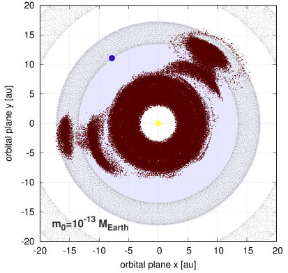
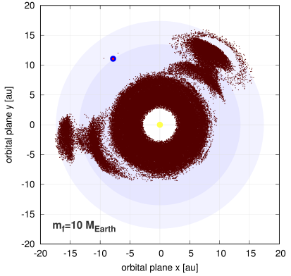
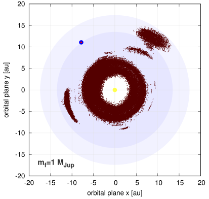
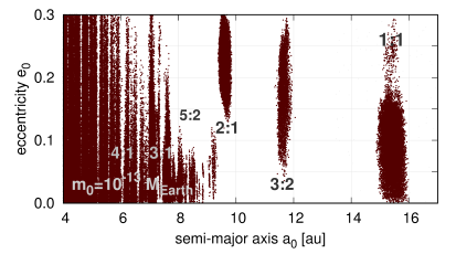
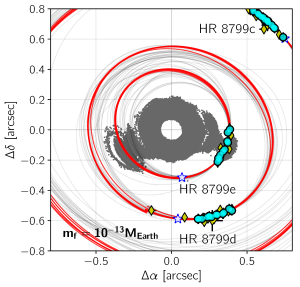
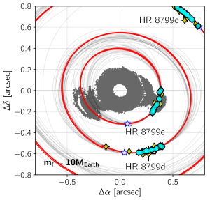
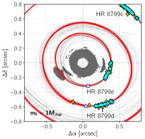
Figure 8: The inner debris disk (the left column) and possible orbits of yet undetected innermost planet HR 8799f (the middle and right columns) in model IV_K at the initial osculating epoch 2004.532. Panels in the top row are for instant astrocentric $(x,y)$ coordinates for different masses of test bodies in stable orbits. The left column is for $10^{-15}\,\mbox{m}_{{\mbox{\scriptsize Jup}}}$, the middle column is for $10$M_Earth, and the right column is for $1$M_Jup, respectively. A filled circle marks the initial position of planet HR 8799e. Light-grey dots in the top-left panel illustrate orbits of two inner planets sampled for the integration time of 3 Myr. For a reference, light-blue discs in two next panels mark the nominal periastron and apoastron distance of HR 8799e. Panels in the middle row are for the $(a_{0},e_{0})$- or $(a_{\rm f},e_{\rm f})$-planes of the initial Keplerian elements with labels identifying low-order MMRs with the innermost planet HR 8799e. Panels in the bottom row are for the $(x,y)$ coordinates rotated to the sky plane, in which the $y$-axis corresponds to N, and the $x$-axis corresponds to E (note the numerical values of $\Delta\alpha$ are sign-opposite to with respect to the formal left-hand direction of the right ascension $\alpha$). Astrometric observations in (Konopacky et al., 2016) are marked with filled circles, and other measurements listed in (Wertz et al., 2017) are marked with diamonds. Several models selected from the MCMC sampling are marked with red (stable, $\chi^{2}_{\nu}\simeq 1$) and grey curves (unstable, $\chi^{2}_{\nu}<0.74$), respectively. For a reference, positions of planets HR 8799c,d,e at the initial epoch of 2004.532 are marked with a star symbol. Note a variability of unstable models, in spite of relatively small $\chi^{2}_{\nu}$. Snapshots in subsequent panels illustrate $\sim 250,000$, $\sim 240,000$ and $\sim 220,000$ $\langle Y\rangle$-stable orbits, respectively, for 3 Myr ($\simeq 6\times 10^{4}$ and $\simeq 3\times 10^{4}$ revolutions of the two closest perturbers HR 8799e,d).

6 The outermost planet V hypothesis

The inner edge of the outer cold debris disk has been detected at $145$ au, hence much farther than $\simeq 90$ au that could be explained by the gravitational pull of planet HR 8799b (Booth et al., 2016; Read et al., 2018). With the same framework and orbital model IV_K of the primaries, as in the previous section regarding the inner disk structure, we aim to investigate locations of a hypothetical fifth planet HR 8799f exterior to HR 8799b. We computed the $\langle Y\rangle$-model for a few choices of the mass $m_{\rm f}$ of the putative planet. The results are illustrated in Fig. 9, for $m_{\rm f}=0.1\,\mbox{m}_{{\mbox{\scriptsize Jup}}}$, $m_{\rm f}=1\,\mbox{m}_{{\mbox{\scriptsize Jup}}}$, and $m_{\rm f}=1.66\,\mbox{m}_{{\mbox{\scriptsize Jup}}}$, respectively, as well as we made a similar experiment for $m_{\rm f}=2.5\,\mbox{m}_{{\mbox{\scriptsize Jup}}}$ (not shown).

The top row in Fig. 9 illustrates possible, stable positions of HR 8799f in the orbital plane at the initial epoch of 2004.532. Again, it should be understood as a representation of the initial conditions implying stable evolution of the system, rather than a physical disk. The distribution of orbits is very similar to that one derived for mass-less or low-mass asteroids shown in Fig. 7. In order to understand the dynamical structure of this quasi-disk, we also plotted the same orbits projected onto the $(a_{\rm f},e_{\rm f})$-plane (the middle-row panels), where $a_{\rm f}$ and $e_{\rm f}$ are the canonical, Poincaré elements (Morbidelli, 2002; Goździewski et al., 2008). This parametrization of the orbital elements is critical to “disentangle” the structure of MMRs. Otherwise, a classification of orbits is obscure with the common, Keplerian astrocentric elements due to significant variation of the osculating semi-major axes of the outer planets (for instance, Lee & Peale, 2003), see also the bottom row in Fig. 6.

As can be deduced from Fig. 9, a Neptune-mass planet could belong to a stable system when involved in a low order 2-body resonance with HR 8799b, like the 1:1, 3:2, 5:3, 2:1 and 5:2 MMRs. In that instance, the eccentricity of the fifth planet could be as large as $e_{\rm f}\simeq 0.3$. It might be found at essentially any location at the sky (see the bottom-row panels), beyond the angular distance roughly equivalent to the semi-major axis of $a_{\rm f}\simeq 90$ au. Also two Trojan, 1:1 MMR locations are possible. A similar, extended yet more sparse and clear pattern of the MMRs is present for a larger mass of $1\,\mbox{m}_{{\mbox{\scriptsize Jup}}}$ (the middle column), as well as for $1.66\,\mbox{m}_{{\mbox{\scriptsize Jup}}}$ (the right column), and $2.5\,\mbox{m}_{{\mbox{\scriptsize Jup}}}$ (not shown).

  

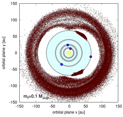
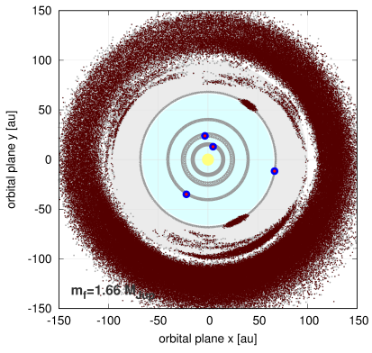
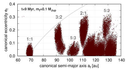
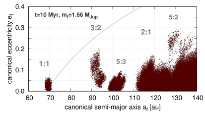
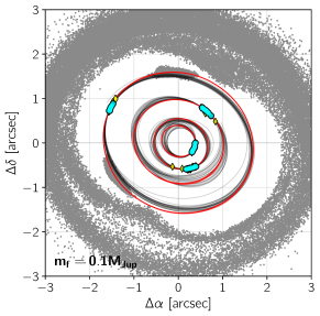
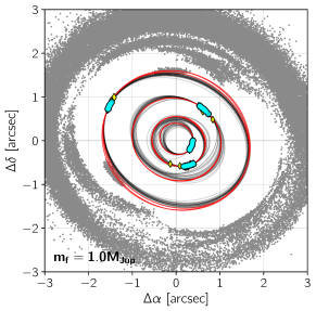
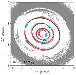
Figure 9: The $\langle Y\rangle$-model simulations of localizations of a putative planet HR 8799f in the outer region of the system. Subsequent panels show astrocentric coordinates $(x,y)$ of stable orbits in the orbital plane (top row), a distribution of the Poincaré canonical orbital elements $(a_{\rm f},e_{\rm f})$ (the middle row) and a projection of the instant coordinates at the sky plane, relative to the observed system (filled circles) and several four-planet synthetic orbits from the MCMC sampling, marked with red and grey curves for stable and unstable models, respectively. The $y$-axis corresponds to N, and the $x$-axis corresponds to E (note that the numerical values of $\Delta\alpha$ are sign-opposite with respect the formal left-hand direction of the right ascension $\alpha$). Columns are for different masses of the putative planet of $0.1\,\mbox{m}_{{\mbox{\scriptsize Jup}}}$, $1\,\mbox{m}_{{\mbox{\scriptsize Jup}}}$ and $1.66\,\mbox{m}_{{\mbox{\scriptsize Jup}}}$, respectively. Light-grey curves in the middle panels indicate the collision curve for planet HR 8799e and test objects. Integrations are done with the $\mu$Farm package with the MEGNO indicator for 9 and 10 Myr. Grey rings in the top panels illustrate sampled orbits of the observed planets for the integration time. The snapshots show up to $2\times 10^{5}$ objects in $\langle Y\rangle$-stable orbits. The reference epoch 2004.532 is the date of the first observation in (Konopacky et al., 2016).

7 The outer debris disk structure

Finally, we conducted $\langle Y\rangle$-model simulations for a few copies of the HR 8799 best-fitting solution, model IV_K in Tab. 1, involving the fifth planet with different masses and the initial semi-major axis. As shown in the previous section, such a planet is weakly constrained by the present astrometry. However, the recent observations of the outer disk imply conjugated constrains for its structure as well as for possible orbit and mass of this putative object.

We aim to simulate the outer disk composed of probe masses $m_{0}$ set to $10^{-15}\,\mbox{m}_{{\mbox{\scriptsize Jup}}}$ in further experiments. After selecting a mass and orbital elements of the fifth, additional planet HR 8799f from simulations described in Sect. 6 and illustrated in Fig. 9, we verified $\langle Y\rangle$ scans in the $(a_{\rm f},e_{\rm f}$)-plane. We checked whether its stability zone is sufficiently wide, to avoid biases due to a proximity to unstable resonances. When necessary, the semi-major axis $a_{\rm f}$ has been slightly modified to separate it safely from all nearby unstable MMRs. The orbital elements of the primaries selected for computations are gathered and labeled in Tab. 1, as HR 8799fA to HR 8799fE, complementing model IV_K. We tested orbits with the initial $a_{0,{\rm k}}\in[60,240]$ au and eccentricities $e_{0,{\rm k}}=[0,\sim 0.5)$ below the collision curve with the outer planet. (For the mass-less particles, we distinguish the Poincaré canonical elements $(a_{\rm p},e_{\rm p})$ from $(a_{0},e_{0})\equiv(a_{\rm k},e_{\rm k})$ denoting common, Keplerian astrocentric elements).

The first set of simulations is illustrated in Fig. 10. Here, we essentially repeated the $\langle Y\rangle$ calibrating experiment in Sect. 4, yet to determine the edge of the outer disk with the updated model IV_K. The ($x,y$) snapshot of stable orbits at the initial osculating epoch of 2004.532 is now complemented with the $(a_{\rm p},e_{\rm p})$-plane for the canonical, Poincaré elements of the orbits of test particles at the end of the integration interval of $10$ Myr, extended to more than $10^{4}$ orbits at $\sim 100$ au. The integration time implies that orbits characterized as $\langle Y\rangle$-stable should be Lagrange-stable for $\simeq 100$ Myr. The $(x,y)$ orbits are coded in a colour-scale representing their initial, Keplerian astrocentric eccentricity $e_{\rm k}$. This provides an additional information on the distribution and geometry of stable orbits at the initial epoch of 2004.532.

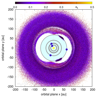
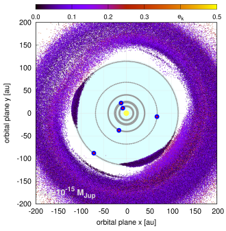
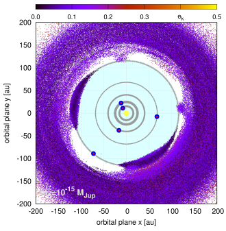
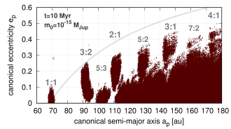
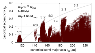
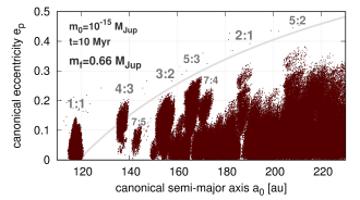
Figure 10: The inner part of the outer debris disk of the four-planet (the left column) and five-planet systems (remaining two columns). Orbital elements of the fifth planet, complementing model IV_K, are listed as HR 8799fA and HR 8799fB, respectively, in Tab. 1. Subsequent panels in the top row show astrocentric coordinates $(x,y)$ of asteroids in $\langle Y\rangle$-stable orbits, for different masses of a hypothetical companion HR 8799f, at the initial epoch of 2004.532. Panels in the bottom row are for the canonical, Poincaré elements $(a_{\rm p},e_{\rm p})$ of these stable solutions at the end of the integration interval of 10 Myr. Grey lines are for the collision curve of orbits with planet HR 8799f. The low-order MMRs with planet HR 8799f are labeled in bottom panels. Osculating, initial orbital eccentricities $e_{\rm k}$ at the initial epoch are color-coded in the top row. Snapshots in subsequent panels illustrate $\sim 920,000$, $\sim 580,000$ and $\sim 910,000$ $\langle Y\rangle$-stable orbits, respectively.

The ($x,y)$-orbital plane shown in the top-left panel in Fig. 10 reveals similar features to those seen in Fig. 7 (the top row). A shape of the inner edge of the disk, resembling a fat peanut, is strongly distorted by orbits of asteroids in the 3:2 and 5:3 MMRs with HR 8799b. They may be easily identified in the $(a_{\rm p},e_{\rm p})$-plot. There are also present large islands of stable particles co-rotating with the $L_{4},L_{5}$ -Lagrangian points of planet b. They extend for wide arcs as long as $\simeq 40$ au. The short-term dynamics in the 100 Myr time-scale is apparently governed by the major gravitational pull of HR 8799b, since stable orbits are possible essentially only below the collision curve $e_{\rm p}(a_{\rm p})$, marked in the bottom row panels in grey. This curve is determined from $a_{\rm b}(1+e_{\rm b})\simeq a_{\rm p}(1-e_{\rm p})$. Some proportion of the asteroids might move on moderately eccentric orbits up to $e_{\rm p}\simeq 0.4$ when trapped in low-order MMRs.

Two next columns in Fig. 10 are for five-planet systems with planet HR 8799fA of mass $m_{\rm f}=1.66\,\mbox{m}_{{\mbox{\scriptsize Jup}}}$ and planet HR 8799fB of mass $m_{\rm f}=0.66\,\mbox{m}_{{\mbox{\scriptsize Jup}}}$, respectively (see model IV_K in Tab. 1). The semi-major axis $a_{\rm f}\sim$116 au, forming the 16e:8d:4c:2b:1f MMR chain, is almost the same in both experiments. These configurations address the inner edge at $\simeq 145$ au, as detected in (Booth et al., 2016). Indeed, for $m_{\rm f}=1.66\,\mbox{m}_{{\mbox{\scriptsize Jup}}}$, stable orbits exhibit semi-major axes $a_{\rm p}>140$ au, beyond Lagrangian $L_{4},L_{5}$ zones, with two strongly resonant regions of the 3:2 and 2:1 MMRs with planet HR 8799f. A similarity of the $(x,y)$ distribution with the results in the bottom panels of Fig. 7 is striking. The inner edge would be strongly distorted by moderately eccentric orbits $e_{\rm p}\simeq 0.2$ associated with the 3:2 MMR. A ring of eccentric 2:1 MMR orbits with $a_{\rm p}\simeq 150$ au is marked with reddish points in top-middle panel. The Lagrangian zones are much wider than in the four planet configuration (panels in the left column of Fig. 10) and extend along arcs of $\sim 100$ au, contributing to even more non-circular and asymmetric inner edge of the disk.

Even more complex inner shape appears for smaller mass $m_{\rm f}=0.66\,\mbox{m}_{{\mbox{\scriptsize Jup}}}$ of the hypothetical planet HR 8799f at $a_{\rm f}\simeq 116$ au (the right column). While the inner edge in the $(a_{\rm p},e_{\rm p})$-plane is similar to the $m=1\,\mbox{m}_{{\mbox{\scriptsize Jup}}}$ case, now the 4:3 MMR is populated with more particles. Also the Lagrange zones are more extended, and moderately eccentric orbits in the 4:3 MMR form two clumps opposite to the planet, at distances equal to its mean heliocentric semi-major axis $a_{\rm f}$. Other features of the asteroids distribution are similar to the previous case.

We also considered an orbital setup with the outer planet f beyond $\simeq 130$ au, as predicted by the disk models in (Booth et al., 2016; Read et al., 2018). Due to the larger semi-major axis of the perturber, the $\langle Y\rangle$ integration time has been increased to 12 Myr ($\sim 10^{4}$ orbits of the outermost perturber at $\sim 130$ au). We investigated three cases with $m_{\rm f}=1\,\mbox{m}_{{\mbox{\scriptsize Jup}}}$, $m_{\rm f}=0.33\,\mbox{m}_{{\mbox{\scriptsize Jup}}}$, and $m_{\rm f}=0.1\,\mbox{m}_{{\mbox{\scriptsize Jup}}}$, respectively, illustrated in columns of Fig. 11. While the overall shape of the disk is roughly similar to the previous models, new features appear. The inner edge becomes more and more distorted from a circle for decreasing masses $m_{\rm f}$. Simultaneously, clumps of stable orbits associated with the Lagrangian equilibria develop to a state in which they are merged with the inner edge at the mean distance equal to the semi-major axis $a_{\rm f}$. Also, the low order MMRs zones are even better isolated, hence the inner edge up to $\simeq 220$ au is strictly resonant.

The most complex image of the inner border of the disk has been found for the smallest mass of $m_{\rm f}=0.1\,\mbox{m}_{{\mbox{\scriptsize Jup}}}$ placed at $a_{\rm f}\simeq 138$ au. This particular configuration follows the best-fitting solution explaining the recent ALMA observations in (Read et al., 2018). The resonant structure associated with this planet is also very sharp, yet some particles may survive in stable, resonant orbits between planets HR 8799b and HR 8799f. We did not find such orbits for $m_{\rm f}=0.33\,\mbox{m}_{{\mbox{\scriptsize Jup}}}$, although planet f is shifted by only $\simeq 5$ au. The inner resonant orbits are associated with 1:1, 3:2 and 5:2 MMRs with planet HR 8799b. In both zones, the eccentricities might be excited beyond collision curves with planets HR 8799b and HR 8799f.

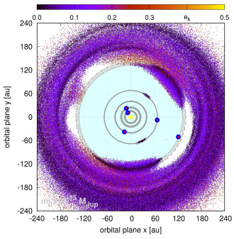
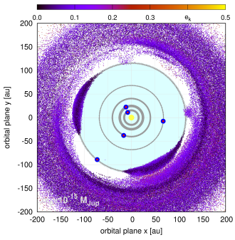
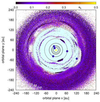
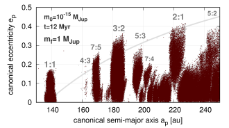
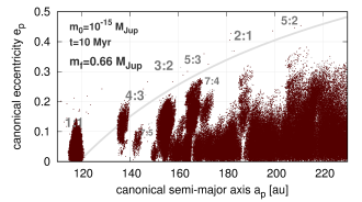
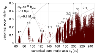
Figure 11: The inner part of the outer debris disk of the five-planet systems and different masses $m_{\rm f}=1\,\mbox{m}_{{\mbox{\scriptsize Jup}}}$, $m_{\rm f}=0.33\,\mbox{m}_{{\mbox{\scriptsize Jup}}}$ and $m_{\rm f}=0.1\,\mbox{m}_{{\mbox{\scriptsize Jup}}}$, respectively, of a hypothetical, fifth planet beyond the orbit of HR 8799b. Orbital elements of the fifth planet, complementing model IV_K, are listed as HR 8799fC, HR 8799fD and HR 8799fE, respectively, in Tab. 1. A mass of this additional planet is labeled at the bottom panels. Subsequent panels in the top row show astrocentric, Cartesian coordinates $(x,y)$ of asteroids at $\langle Y\rangle$-stable orbits, for different masses $m_{\rm f}$ of a hypothetical companion HR 8799f labeled in subsequent bottom panels, at the initial epoch of 2004.532. Panels in the bottom row are for the canonical, Poincaré elements of these stable solutions at the end of the integration intervals of 10 Myr and 12 Myr. Grey lines are for collision curves of orbits with planet HR 8799f, and also with planet HR 8799b (the right column). Low-order MMRs with planet HR 8799f, and with planet HR 8799b are labeled. Osculating astrocentric eccentricities $e_{\rm k}$ at the initial epoch are color-coded in panels at the top row. Snapshots in subsequent panels illustrate $\sim 980,000$, $\sim 635,000$ and $\sim 500,000$ $\langle Y\rangle$-stable orbits, respectively.

8 The debris disc under migration

The resonant nature of the four known planet configuration might result from the migration due to the planet-disc interactions. Including this process in the debris disc formation scenario may potentially shift the border with respect to the results of the previously studied models in which all the planets are statically placed at their current orbits together with a disc of the mass-less particles. We therefore aim to investigate whether migration of the planets might place the inner edge of the outer debris belt at $\sim 145$ au. Then the requirement for an additional planet outside the orbit of planet b could be released. While the analysis is preliminary, it might offer an alternative scenario for explaining the ALMA observations.

We assume that the planets are initially located outside their current positions and they undergo the inward convergent migration that is supposed to form a chain of 2:1 MMRs. We use the same model of the planet-disc interactions, as used before and described by Eq. 1, yet with $\kappa$ the same for all planets.

Although the mass-less particles are too small to undergo the type I migration, they could, in principle, “feel”’ the gas drag (Adachi et al., 1976). The timescales of the orbit decay that results from the drag depends strongly on the particles masses as well as on the gas densities (the volume densities, not the surface densities as for the type I and type II migration). Assuming that the surface gas density $\propto r^{-3/2}$ and the total gas mass within the $(10,100)\,\mbox{au}$ range equals $1\,\,\mbox{m}_{{\mbox{\scriptsize Jup}}}$ when we start the simulation, the volume gas density would be in a range of $10^{-14}$ and $10^{-15}$g/cm³, depending on the assumed aspect ratio between $0.01$ and $0.1$. For particles larger than a meter the characteristic timescale of the orbit decay induced by the gas drag would be greater than the age of the system, and greater that the migration timescales assumed for the planets, that are $\sim 10$Myr. Therefore, we neglect the migration of the mass-less particles in this model.

We performed a series of simulations for different initial orbits and the migration parameters. We assume that the resulting system has to be resonant, of a similar size as the observed configuration and the inner edge of the mass-less particles disc has to place in the range of $(145\pm 12)\,\mbox{au}$ as determined by Booth et al. (2016). These constrains do not permit for very wide initial orbits, since the resulting inner edge would be placed outside the observed border. On the other hand, all the pairs of planets need to be located outside 2:1 MMRs, as the resonances are formed in the process of the convergent migration. Moreover, the innermost planet should start the migration beyond its current position at $\sim 15.5\,\mbox{au}$.

All the constrains given above limit the initial orbits significantly. After a series of experiments we found an initial configuration and the migration parameters that fulfills the criteria. The evolution of the four-planet system into the resonant configuration is shown in the left-hand column of Fig. 12. The initial semi-major axes and other parameters are given in the caption of the figure. The outermost planet starts the migration at $90\,\mbox{au}$, while the innermost one at $17.5\,\mbox{au}$. The migration timescales between $9$ and $28$ Myr (from the outermost to the innermost planets, respectively) together with the disc decay timescale of $1~{}$Myr make the planets to migrate inwards by a distance of $\sim 20\,\mbox{au}$ for the outermost and $\sim 2\,\mbox{au}$ for the innermost planets. The resonance (with low-amplitude libration of the resonant angle) is formed after $\sim 1~{}$Myr of the evolution, therefore the final system of four planets is long-term stable.

The process of the resonant chain formation needs a comment. Entering into the resonant chain of four planets is a chaotic process, therefore even small changes in the initial configuration as well as differences between the numerical integrators used to solve the equations of motion may lead to different results, for instance the resonance could be not achieved, resulting in further self-disruption of the system. This is why the evolution shown here has to be treated as an example configuration. Initial configurations different to the one presented as well as different migration parameters may lead to qualitatively similar results.

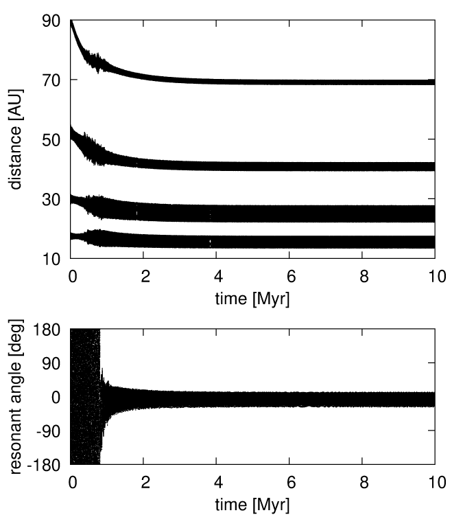
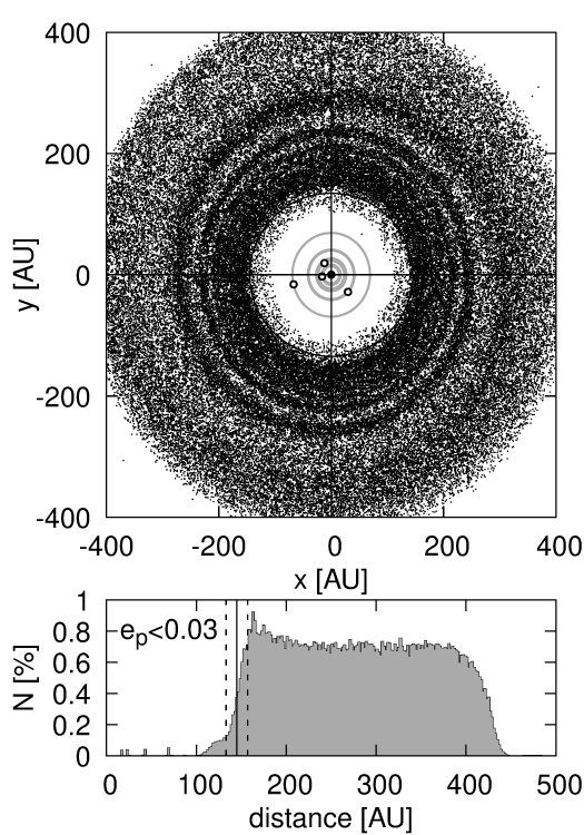
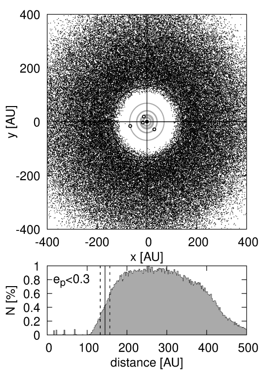
Figure 12: The left-hand column: Evolution of an example initial configuration that ends up as a system resembling the configuration of the HR 8799. Initial semi-major axes are $a_{1}=17.5\,\mbox{au},a_{2}=30\,\mbox{au},a_{3}=52\,\mbox{au}$ and $a_{4}=90\,\mbox{au}$. All eccentricities and arguments of pericenters are initially $0$. Mean anomalies are chosen to be $0,90,180$ and $170$ degrees, from the innermost to the outermost planets respectively. The migration parameters are $T=1~{}$Myr, $\kappa=200$ and respective timescale of migration $\tau_{1}=28~{}$Myr, $\tau_{2}=18~{}$Myr, $\tau_{3}=12~{}$Myr, $\tau_{4}=9~{}$Myr. The masses are the same as in solution IVa in (Goździewski & Migaszewski, 2014, see also Tab. 1), i.e., $m_{\star}=1.56\,\mbox{M}_{\odot}$, $m_{1}=m_{2}=m_{3}=9\,\,\mbox{m}_{{\mbox{\scriptsize Jup}}}$, $m_{4}=7\,\,\mbox{m}_{{\mbox{\scriptsize Jup}}}$. The top panel presents the evolution of the astrocentric distances of the planets, while the bottom panel illustrates the evolution of the resonant angle of the double Laplace resonance, i.e., $\theta=\lambda_{1}-2\lambda_{2}-\lambda_{3}+2\lambda_{4}$. The middle and right-hand columns: Final distribution of asteroids after $10$ Myr of evolution. The top panels present the position of asteroid in the orbital plane (dots), together with the positions of the planets (big dots). Gray rings show the temporal positions of the planets integrated over $100~{}$Myr after the migration stops. Black circle points the inner border of the outer debris disc of HR 8799 found in (Booth et al., 2016), i.e., $145\,\mbox{au}$. Bottom panels present histograms of the asteroids’ astrocentric distances. Vertical lines indicate the debris disc border (solid line) together with the uncertainties (dashed lines), i.e., $(145\pm 12)\,\mbox{au}$. The initial asteroids’ eccentricities were chosen from the ranges of $[0,0.03]$ (the middle column) and $[0,0.3]$ (the right column).

Apart from the planets, there is a number of mass-less objects included in the model, whose motion is being perturbed by the planets. Their final distribution after $10$ Myr of the integration is shown in the middle and the right-hand columns of Fig. 12. We chose a uniform distribution of the particles semi-major axes, ranging from $15\,\mbox{au}$ to $429\,\mbox{au}$ (the latter is the outer edge of the debris belt found by Booth et al., 2016). Initial eccentricities of the particles ranges from $0$ to $0.03$ (the middle column) and from $0$ to $0.3$ (the right-hand column), all the angles are chosen randomly in the whole range of $(0^{\circ},360^{\circ})$. The final number of objects that remained in the system $\sim 10^{5}$ in each case. The inner edge of the asteroids belt places itself at $\sim 145\,\mbox{au}$ for both ranges of the initial eccentricities. The border is more sharp for the simulations with initial $e<0.03$. Moreover, in this case there are spiral waves in the disc, while when initial $e<0.3$ the disc is axially symmetric.

In both the cases, there is a small number of objects inside $145\,\mbox{au}$, that results from non-rectangular radial distribution of the asteroids. We fine-tuned the initial orbits of the giant planets in such a way that at the distance of $145\,\mbox{au}$ the radial density of the object equals approximately half of the radial density in the plateau region of the radial distribution. The border defined in this way can be easily controlled when the model with migration is applied, simply by shifting initial positions of the planets, as most of the asteroid are being removed from the system shortly after the beginning of the simulation, when the giant planets are still close to their initial positions.

9 Discussion

Our results are derived under the major assumption that the orbital models of the HR 8799 systems are resonant, and the strong, zero-th Laplace MMR chain is likely the primary factor maintaining the long-term stability. However, some recent results in the literature might apparently contradict this assumption, which possibly requires a comment.

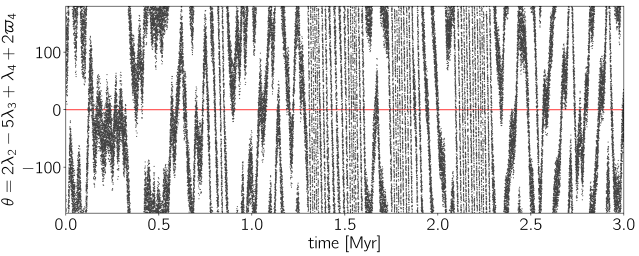
Figure 13: Temporal evolution of a critical argument $\theta$ of the three-body 2d:-5e:1b MMR of the system 94, simulation 4e in (Götberg et al., 2016, their Appendix). A sequence of alternating librations and rotations implies separatrix crossings and strongly chaotic evolution of the system.

Recently, Götberg et al. (2016) proposed long-term Lagrange-stable solutions found by tuning the initial orbital separations between the planets in terms of the Hill-radii spacing (Chatterjee et al., 2008). These long-living models are reported as non-resonant, strongly chaotic and prone to tiny changes of the initial conditions and a numerical scheme.

We examined system 94 (simulation 4e) in Appendix of the source paper, given in the form of Cartesian, astrocentric coordinates. The frequency analysis of this solution reveals that it exhibits alternating rotations and librations of a critical argument of the three-body MMR 2d:-5c:1b (Fig. 13). This feature indicates the separatrix crossing. We also did 2-dim $\langle Y\rangle$-scans in the $(a_{\mbox{\scriptsize\rm e}},e_{{\mbox{\scriptsize\rm e}}})$-plane, close to this solution (not shown), which reveal a dense net of other narrow multi-body MMRs in this region around $a_{{\mbox{\scriptsize\rm e}}}\simeq 14.3$ au. The scans might be helpful to select other marginally stable solutions associated with narrow three-body and four-body MMRs of higher orders.

The results of Götberg et al. (2016) are consistent with our simulations in the sense that they indicate a marginal stability of the system. It may be long living only in very narrow stability regions in the phase space, associated with various multi-body MMRs. A resonance mechanism protecting the system from close encounters must be acting for the present planetary mass estimates, though the orbital evolution may be chaotic and marginally stable, as we also argue in (Goździewski & Migaszewski, 2009, 2014), and in this work.

A determination of the Hill-radii separation through semi-major axes expressed in astrocentric reference frame may be non-unique. For instance, the semi-major axis of HR 8799b in the model 94 (simulation 4e) in (Götberg et al., 2016) varies within $10$ au, depending on the orbital phase, although the orbit has been set initially almost circular. It may be explained by indirect perturbations in the astrocentric frame, see (Lee & Peale, 2003) for details; also this work, regarding identification of MMRs in the outer debris disk (Sects. 6 and 7). The osculating period of HR 8799b simultaneously varies roughly between 450 and 550 years that hinders the proper identification of the MMRs. The identification is much easier in the canonical reference frame. In that frame the $N$-body dynamics may be approximated to the first order in the masses through the Keplerian orbits perturbed by the mutual interactions between the planets (e.g., Malhotra, 1993).

A choice of the astrometric model is one more subtle, yet crucial factor for determining the long-term stable solutions. By reproducing the observations with Keplerian orbits, we dismiss information on the planet masses. Apparently, the mutual interactions should not be a significant factor for resolving the orbital geometry given that the observed arcs are at most $\sim 12\%$ of the full orbits. However, the masses are critical for determining the dynamical interactions in the system, hence skipping this prior seems to be inconsistent with the Bayesian inference. Even rigorously stable $N$-body models exhibit orbits which do not close after just one osculating period (Sect. 3). Unstable models marginally worse from mathematically best-fitting solutions are unconstrained and represent widely open arcs during only one osculating period (Fig. 6). These arguments indicate that the kinematic (geometric) models may be already biased, in spite of the short-arc measurements coverage.

10 Summary

In the first part of the paper, we present an updated astrometric model of the HR 8799 planetary system. If the masses of detected planets are in a few Jupiter mass range, the system is strongly unstable in 1 Myr time-scale. It is still a very short interval of time, when compared to the star age, estimated between 30 and 160 Myr. Simulations of its dynamics conducted so far reveal that the long-term stable orbital architectures of the system must be confined to small and particular regions in the phase space. We attempt to solve this paradox by assuming that the HR 8799 system is involved in a 2-body MMR chain or multiple, three- or four-body MMR. Since the orbital parameters of a stable, resonant configuration are not independent and coupled, the number of free parameters of the astrometric model may be reduced to only five. This makes it possible to find stable solutions consistent with astrometric measurements and mass estimates derived from the planet formation and cooling theory.

While the original version of this optimization method has been developed earlier, in this work we propose a structured and CPU-efficient algorithm that consists of two independent steps. At the first stage we build a database of stable configurations by simulating the planetary migration process. These synthetic, co-planar systems may agree only roughly with the spatial dimensions of the observed system. The second step performed with evolutionary algorithms is for fine-tuning these systems through the linear scaling, rotations of the orbits in space and propagating the bodies along their orbits with the $N$-body code to the proper, observed positions. We note that during the latter step, the elements may change self-consistently, in accord with the $N$-body evolution.

This approach lead us to finding the best-fitting model with $\chi^{2}_{\nu}\simeq 1$, which corresponds to the MMR chain of a generalized, four-body Laplace resonance. This solution to a subset of self-consistent astrometric measurements in (Konopacky et al., 2016) extrapolates to all observations to date and preserves the correct timing. In particular, the extrapolated orbit of planet HR 8799d passes closely to the first HST observation in 1998 (Lafrenière et al., 2009). Solutions unconstrained by the migration are widely spread, in spite of much smaller $\chi^{2}_{\nu}\sim 0.74$, only marginally worse from mathematically best-fitting configuration yielding $\chi^{2}_{\nu}\sim 0.6$. It may be a strong argument supporting our resonant model. Also the mutual gravitational interactions between the planets are apparent since the best-fitting $N$-body orbits may collide in a time-scale of a few revolutions. That puts in concern kinematic models that do not account for the mutual interactions between the planets.

In the second part, we used the stable best-fitting initial conditions for simulating the dynamical structure of debris disks in the system. We developed CPU-efficient sampling of the initial conditions with the fast indicator MEGNO, dubbed as the $\langle Y\rangle$-model. This dynamical model makes it also possible to locate additional, relatively massive objects in stable orbits, representing yet undetected planets in the system. The HR 8799 system of four planets involved in the Laplace 8b:4c:2d:1e MMR is surprisingly robust for relatively strong perturbations introduced by such additional objects in 1-3 Jupiter mass range. Such unknown planets may be found interior or exterior to planets HR 8799e and HR 8799b, respectively, and extending the MMR chain to five or more planets.

With the $\langle Y\rangle$-model, we simulated the debris disks composed of small asteroids. The structure of these disks is represented by temporal coordinates in the orbital plane, as well as by the canonical Keplerian elements in the $(a_{\rm p},e_{\rm p})$-plane. The simulations ended up with $\sim 10^{6}$ particles, and reveal regions which may be populated by asteroids or small planets in stable orbits. The total number of tested initial conditions was one-two orders of magnitude larger when counting unstable solutions. The $\langle Y\rangle$-model was calibrated with the long-term, direct numerical integrations performed with the standard Mercury 6.3 code. The results for the four- and five-planet restricted problems derived with the direct numerical integrations for 34-68 Myr closely overlap with outcomes from the $\langle Y\rangle$-model traced for much shorter intervals of $7$–$12$ Myr.

The outer edge of the inner disk is shaped mostly by the inner planet e. A border of stable motions may be roughly determined by the collision zone with this planet. Close to its orbit, stable orbits are permitted only when asteroids or small-mass objects are trapped in low-order MMRs. The overall image of this zone is similar for a range of masses, between $10^{-15}\,\mbox{m}_{{\mbox{\scriptsize Jup}}}$ (small asteroids) and $1\,\mbox{m}_{{\mbox{\scriptsize Jup}}}$ (Jovian planets). By allowing for the initial eccentricities of the test bodies up to the limit determined by collisional orbits, we detected stable resonances, like 3:2 and 1:1 MMRs missing in earlier papers (Contro et al., 2016). The presence of a significant proportion of asteroids in these resonances may contribute to highly non-symmetric edge of the inner disk.

We also conducted CPU-intensive simulations of the outer disk, focusing on its inner edge and the inner part. Recently, it has been resolved with the ALMA observations in band 6 (1.34 mm) by Booth et al. (2016) and combined ALMA and VLA observations by Wilner et al. (2018). They found the inner edge at 145$\pm 12$ au and 104${}^{+8}_{-12}$ au, respectively. Followup, extensive simulations by (Read et al., 2018) focus on the fifth, undetected planet carving the outer disk, to be consistent with the model of Booth et al. (2016). Their best fitting model predicts a small 0.1$\,\mbox{m}_{{\mbox{\scriptsize Jup}}}$ planet at $\simeq 138$ au. However, a different model in (Wilner et al., 2018) may explain the ALMA and VLA observations with the currently observed four-body system. They also constrained a mass of planet HR 8799b to 5.8${}^{+7.9}_{-3.1}$ au.

We reconstructed the inner part of the disk composed of low-mass particles (asteroids) under different dynamical conditions, covering scenarios in these three papers, in the framework of the four- and five-planet restricted problem.

The inner edge is mostly influenced by the outermost planet. The simulations ended up with $10^{6}$ bodies in stable orbits. The inner part of the outermost disk is spanned with various MMRs with this planet, including the 1:1 MMR and extended co-rotation zones. The width of these zones depends on the outermost planets’ mass, and may extend for $\sim 100$ au. A border of stability region beyond the orbit of the outermost planet HR 8799b is determined by the collision zone with this planet. Low order resonances, like the 4:3, 3:2 and 2:1 MMR force eccentricity of the asteroids to moderate values. If these stable, moderate-eccentricity regions are populated, then the inner edge may exhibit very complex shape. It turns out to be more asymmetric for smaller masses of the outermost planet. We found the most complex edge for 0.1$\,\mbox{m}_{{\mbox{\scriptsize Jup}}}$ at $\sim 138\,\mbox{m}_{{\mbox{\scriptsize Jup}}}$, predicted in the best-fitting model to the ALMA observations in (Read et al., 2018).

We note that in papers modeling the ALMA data, the edge is axi-symmetric with inclusion of the Lagrangian clumps appearing as non-important for the final results. However, our simulations indicate that the inner edge may be irregular, and particularly the 1:1 MMR zones overlapping with eccentric orbits in 3:2 and 4:3 MMRs may produce extended regions of emission. For instance, 0.33 $\,\mbox{m}_{{\mbox{\scriptsize Jup}}}$ planet placed at $\sim 134$ au would be responsible for maintaining two huge Lagrangian clumps spanning approximately $120\times 30$ au each. A smaller planet $\sim 0.1\,\mbox{m}_{{\mbox{\scriptsize Jup}}}$ beyond $\sim 135$ au might permit a complex structure of stable motions interior to its orbit and confined to low order MMRs with HR 8799b.

Finally, we tentatively simulated the migration of the four observed planets in the presence of an extended asteroidal belt. We assume that the planets migrate to the final state of the 8b:4c:2d:1e Laplace resonance and influence the asteroids. In this most complex astrophysical scenario, the disk edge may be moved to a “desired” location by appropriate migration rates and initial configuration of the planets. In such a case no additional planets would be necessary in order to explain the ALMA observations. These simulations have a dynamic character, contrary to the static case considered in previous experiments. However, the static-type simulations made with the observed four-planet system are still complementary to the migration scenario. They reconstruct a detailed disk structure after the gaseous component has been dispersed, and the planet migration has slowed down or stopped. In particular, they reveal the dynamical structure of less populated regions between $\sim 90$ and $150$ au.

We conclude that the HR 8799 dynamical state cannot be yet fully resolved. While our resonant model may explain the astrometric observations, a longer time coverage is required to determine the real orbits without any doubt. As we confirm in this work, high-resolution images and observations of the debris disks may introduce additional, though indirect limits on the HR 8799 system architecture. Various factors may be responsible for shaping the debris disks, like the presence of undetected planets, their masses and orbits. Therefore interpretation of the spectral energy distributions (SEDs) and the spatial disk imaging seems to be a complex and difficult problem, as the debris disk models may be non-unique. Our results and followup dynamical simulations, similar to those made in our paper, could be helpful to reduce this indeterminacy.

References

- Adachi et al. (1976) Adachi, I., Hayashi, C., & Nakazawa, K. 1976, Progress of Theoretical Physics, 56, 1756
- Armitage (2018) Armitage, P. J. 2018, ArXiv e-prints, 1803.10526, arXiv:1803.10526
- Baines et al. (2012) Baines, E. K., White, R. J., Huber, D., et al. 2012, ApJ, 761, 57
- Baraffe et al. (2003) Baraffe, I., Chabrier, G., Barman, T. S., Allard, F., & Hauschildt, P. H. 2003, A&A, 402, 701
- Beaugé et al. (2006) Beaugé, C., Michtchenko, T. A., & Ferraz-Mello, S. 2006, MNRAS, 365, 1160
- Bergfors et al. (2011) Bergfors, C., Brandner, W., Janson, M., Köhler, R., & Henning, T. 2011, A&A, 528, A134
- Bevington & Robinson (2003) Bevington, P. R., & Robinson, D. K. 2003, Data reduction and error analysis for the physical sciences (McGraw-Hill, Boston)
- Booth et al. (2016) Booth, M., Jordán, A., Casassus, S., et al. 2016, MNRAS, 460, L10
- Chambers (1999) Chambers, J. E. 1999, MNRAS, 304, 793
- Chambers et al. (1996) Chambers, J. E., Wetherill, G. W., & Boss, A. P. 1996, Icarus, 119, 261
- Charbonneau (1995) Charbonneau, P. 1995, The Astrophysical Journal Supplement Series, 101, 309
- Chatterjee et al. (2008) Chatterjee, S., Ford, E. B., Matsumura, S., & Rasio, F. A. 2008, ApJ, 686, 580
- Cincotta et al. (2003) Cincotta, P. M., Giordano, C. M., & Simó, C. 2003, Physica D Nonlinear Phenomena, 182, 151
- Cincotta & Simó (2000) Cincotta, P. M., & Simó, C. 2000, A&A Suppl. Ser., 147, 205
- Contro et al. (2016) Contro, B., Horner, J., Wittenmyer, R. A., Marshall, J. P., & Hinse, T. C. 2016, MNRAS, 463, 191
- Currie (2016) Currie, T. 2016, ArXiv e-prints, arXiv:1607.03980
- Currie et al. (2012) Currie, T., Fukagawa, M., Thalmann, C., Matsumura, S., & Plavchan, P. 2012, ApJL, 755, L34
- Currie et al. (2011) Currie, T., Burrows, A., Itoh, Y., et al. 2011, ApJ, 729, 128
- de Souza Torres & Anderson (2008) de Souza Torres, K., & Anderson, D. R. 2008, ArXiv e-prints, arXiv 0808.0483:0808.0483
- Esposito et al. (2013) Esposito, S., Mesa, D., Skemer, A., et al. 2013, A&A, 549, A52
- Fabrycky & Murray-Clay (2010) Fabrycky, D. C., & Murray-Clay, R. A. 2010, ApJ, 710, 1408
- Foreman-Mackey et al. (2013) Foreman-Mackey, D., Hogg, D. W., Lang, D., & Goodman, J. 2013, PASP, 125, 306
- Gaia Collaboration et al. (2018) Gaia Collaboration, Brown, A. G. A., Vallenari, A., et al. 2018, ArXiv e-prints 1804.09365, arXiv:1804.09365
- Galicher et al. (2011) Galicher, R., Marois, C., Macintosh, B., Barman, T., & Konopacky, Q. 2011, ApJL, 739, L41
- Götberg et al. (2016) Götberg, Y., Davies, M. B., Mustill, A. J., Johansen, A., & Church, R. P. 2016, A&A, 592, A147
- Goździewski et al. (2008) Goździewski, K., Breiter, S., & Borczyk, W. 2008, MNRAS, 383, 989
- Goździewski & Migaszewski (2009) Goździewski, K., & Migaszewski, C. 2009, MNRAS, 397, L16
- Goździewski & Migaszewski (2014) —. 2014, MNRAS, 440, 3140
- Hadden & Lithwick (2018) Hadden, S., & Lithwick, Y. 2018, AJ, arXiv:1803.08510
- Hairer et al. (2002) Hairer, E., Wanner, G., & Lubich, L. 2002, Geometric Numerical Integration: Structure-Preserving Algorithms for Ordinary Differential Equations, 2nd edn., Springer Series in Computational Mathematics 31 (Springer Berlin Heidelberg)
- Hinkley et al. (2011) Hinkley, S., Carpenter, J. M., Ireland, M. J., & Kraus, A. L. 2011, ApJL, 730, L21
- Hinz et al. (2010) Hinz, P. M., Rodigas, T. J., Kenworthy, M. A., et al. 2010, ApJ, 716, 417
- Izzo et al. (2012) Izzo, D., Ruciński, M., & Biscani, F. 2012, The Generalized Island Model, Vol. 415 (Berlin, Heidelberg: Springer-Verlag), 151–169
- Konopacky et al. (2016) Konopacky, Q. M., Marois, C., Macintosh, B. A., et al. 2016, AJ, 152, 28
- Lafrenière et al. (2009) Lafrenière, D., Marois, C., Doyon, R., & Barman, T. 2009, ApJL, 694, L148
- Laskar (1993) Laskar, J. 1993, Celestial Mechanics and Dynamical Astronomy, 56, 191
- Laskar & Robutel (2001) Laskar, J., & Robutel, P. 2001, Celestial Mechanics and Dynamical Astronomy, 80, 39
- Lee & Peale (2003) Lee, M. H., & Peale, S. J. 2003, The Astrophysical Journal, 592, 1201
- Maire et al. (2015) Maire et al., A. L. 2015, A&A, 579, doi:10.1051/0004-6361/201425185e
- Malhotra (1993) Malhotra, R. 1993, ApJ, 407, 266
- Malhotra (1998) Malhotra, R. 1998, in Solar System Formation and Evolution: ASP Conference Series, Vol. 149, 1998, ed. D. Lazzaro; R. Vieira Martins; S. Ferraz-Mello; J. Fernandez; and Beauge, p.37, Vol. 149, 37
- Marleau & Cumming (2014) Marleau, G.-D., & Cumming, A. 2014, MNRAS, 437, 1378
- Marois et al. (2008) Marois, C., Macintosh, B., Barman, T., et al. 2008, Science, 322, 1348
- Marois et al. (2010) Marois, C., Zuckerman, B., Konopacky, Q. M., Macintosh, B., & Barman, T. 2010, Nature, 468, 1080
- Marshall et al. (2010) Marshall, J., Horner, J., & Carter, A. 2010, International Journal of Astrobiology, 9, 259
- Matthews et al. (2014) Matthews, B., Kennedy, G., Sibthorpe, B., et al. 2014, ApJ, 780, 97
- Metchev et al. (2009) Metchev, S., Marois, C., & Zuckerman, B. 2009, ApJL, 705, L204
- Moore et al. (2013) Moore, A., Hasan, I., & Quillen, A. C. 2013, MNRAS, 432, 1196
- Morbidelli (2002) Morbidelli, A. 2002, Modern celestial mechanics : aspects of solar system dynamics (CRC Press, Advances in Astronomy and Astrophysics)
- Moro-Martín et al. (2010) Moro-Martín, A., Malhotra, R., Bryden, G., et al. 2010, ApJ, 717, 1123
- Morrison & Kratter (2016) Morrison, S. J., & Kratter, K. M. 2016, ApJ, 823, 118
- Oppenheimer et al. (2013) Oppenheimer, B. R., Baranec, C., Beichman, C., et al. 2013, ApJ, 768, 24
- Panichi et al. (2017) Panichi, F., Goździewski, K., & Turchetti, G. 2017, MNRAS, 468, 469
- Papaloizou (2015) Papaloizou, J. C. B. 2015, International Journal of Astrobiology, 14, 291
- Papaloizou & Terquem (2006) Papaloizou, J. C. B., & Terquem, C. 2006, Reports on Progress in Physics, 69, 119
- Price et al. (2005) Price, K., Storn, R. M., & Lampinen, J. A. 2005, Differential Evolution: A Practical Approach to Global Optimization (Natural Computing Series) (Berlin, Heidelberg: Springer-Verlag)
- Pueyo et al. (2015) Pueyo et al., L. 2015, ApJ, 803, doi:10.1088/0004-637X/803/1/31
- Read et al. (2018) Read, M. J., Wyatt, M. C., Marino, S., & Kennedy, G. M. 2018, MNRAS, arXiv:1801.06513
- Reidemeister et al. (2009) Reidemeister, M., Krivov, A. V., Schmidt, T. O. B., et al. 2009, A&A, 503, 247
- Šidlichovský & Nesvorný (1996) Šidlichovský, M., & Nesvorný, D. 1996, Celestial Mechanics and Dynamical Astronomy, 65, 137
- Skemer et al. (2012) Skemer, A. J., Hinz, P. M., Esposito, S., et al. 2012, ApJ, 753, 14
- Sokal (1996) Sokal, A. D. 1996, in Lectures at the Cargése Summer School on Functional Integration: Basics and Applications, Vol. http://www.stat.unc.edu/faculty/cji/Sokal.pdf, 76
- Soummer et al. (2011) Soummer, R., Brendan Hagan, J., Pueyo, L., et al. 2011, ApJ, 741, 55
- Su et al. (2009) Su, K. Y. L., Rieke, G. H., Stapelfeldt, K. R., et al. 2009, ApJ, 705, 314
- Sudol & Haghighipour (2012) Sudol, J. J., & Haghighipour, N. 2012, ApJ, 755, 38
- van Leeuwen & Fantino (2005) van Leeuwen, F., & Fantino, E. 2005, A&A, 439, 791
- Wertz et al. (2017) Wertz, O., Absil, O., Gómez González, C. A., et al. 2017, A&A, 598, A83
- Wilner et al. (2018) Wilner, D. J., MacGregor, M. A., Andrews, S. M., et al. 2018, ApJ, 855, 56
- Zurlo et al. (2016) Zurlo et al., A. 2016, A&A, 587, doi:10.1051/0004-6361/201526835