A Distributed Collaborative Filtering Algorithm Using Multiple Data Sources

A Distributed Collaborative Filtering Algorithm Using Multiple Data Sources

Abstract

Collaborative Filtering (CF) is one of the most commonly used recommendation methods. CF consists in predicting whether, or how much, a user will like (or dislike) an item by leveraging the knowledge of the user’s preferences as well as that of other users. In practice, users interact and express their opinion on only a small subset of items, which makes the corresponding user-item rating matrix very sparse. Such data sparsity yields two main problems for recommender systems: (1) the lack of data to effectively model users’ preferences, and (2) the lack of data to effectively model item characteristics. However, there are often many other data sources that are available to a recommender system provider, which can describe user interests and item characteristics (e.g., users’ social network, tags associated to items, etc.). These valuable data sources may supply useful information to enhance a recommendation system in modeling users’ preferences and item characteristics more accurately and thus, hopefully, to make recommenders more precise. For various reasons, these data sources may be managed by clusters of different data centers, thus requiring the development of distributed solutions. In this paper, we propose a new distributed collaborative filtering algorithm, which exploits and combines multiple and diverse data sources to improve recommendation quality. Our experimental evaluation using real datasets shows the effectiveness of our algorithm compared to state-of-the-art recommendation algorithms.

I Introduction

Nowadays, Internet floods users with useless information. Hence, recommender systems are useful to supply them with content that may be of interest. Recommender systems have become a popular research topic over the past 20 years, to make them more accurate and effective along many dimensions (social dimension [1][2][3], geographical dimension [4][5], diversification aspect [6][7][8], etc.).

Collaborative Filtering (CF) [9] is one of the most commonly used recommendation methods. CF consists in predicting whether, or how much, a user will like (or dislike) an item by leveraging the knowledge of the user preferences, as well as that of other users. In practice, users interact and express their opinions on only a small subset of items, which makes the corresponding user-item rating matrix very sparse. Consequently, in a recommender system, this data sparsity induces two main problems: (1) the lack of data to effectively model user preferences (new users suffer from the cold-start problem [10]), and (2) the lack of data to effectively model items characteristics (new items suffer from the cold-start problem since no user has yet rated them).

On the other hand, beside this sparse user-item rating matrix, there are often many other data sources that are available to a recommender system, which can provide useful information that describe user interests and item characteristics. Examples of such diverse data sources are numerous: a user social network, a user’s topics of interest, tags associated to items, etc. These valuable data sources may supply useful information to enhance a recommendation system in modeling user preferences and item characteristics more accurately and thus, hopefully, to make more precise recommendations. Previous research work has demonstrated the effectiveness of using external data sources for recommender systems [1][2][3]. However, most of the proposed solutions focus on the use of only one kind of data provided by an online service (e.g., social network in [1] or geolocation information in [4][5]). Extending these solutions into a unified framework that considers multiple and diverse data sources is itself a challenging research problem.

Furthermore, these diverse data sources are typically managed by clusters at different data centers, thus requiring the development of new distributed recommendation algorithms to effectively handle this constantly growing data. In order to make better use of these different data sources, we propose a new distributed collaborative filtering algorithm, which exploits and combines multiple and diverse data sources to improve recommendation quality. To the best of our knowledge, this is the first attempt to propose such a distributed recommendation algorithm. In summary, the contributions of this paper are:

1. A new recommendation algorithm, based on matrix factorization, which leverages multiple and diverse data sources. This allows better modeling user preferences and item characteristics.

2. A distributed version of this algorithm that mainly computes factorizations of matrices by exchanging intermediate latent feature matrices in a coordinated manner.

3. A thorough comparative analysis with state-of-the-art recommendation algorithms on different datasets.

This paper is organized as follows: Section II provides two use cases; Section III presents the main concepts used in this paper; Section IV describes our multi-source recommendation model; Section V gives our distributed multi-source recommendation algorithm; Section VI describes our experimental evaluation; Section VII discusses the related work; Finally, Section VIII concludes and provides future directions.

II Use Cases

Let us illustrate our motivation with two use cases, one with internal data sources, one with external data sources.

II-A Diverse internal data sources

Consider John, a user who has rated a few movies he saw on a movie recommender system. In that same recommendation system, John also expressed his topics of interest regarding movie genres he likes. He also maintains a list of friends, which he trusts and follows to get insight on interesting movies. Finally, John has annotated several movies he saw, with tags to describe their contents.

In this example, the same recommender system holds many valuable data sources (topics of interest, friends list, and annotations), which may be used to accurately model John’s preferences and movies’ characteristics, and thus, hopefully to make more precise recommendations. In this first scenario, we suppose that these diverse data sources are hosted over different clusters of the same data center of the recommender system. It is obvious that a centralized recommendation algorithm induces a massive data transfer, which will cause a bottleneck problem in the data center. This clearly shows the importance of developing a distributed recommendation solution.

II-B Diverse external data sources

Let us now consider that John is a regular user of a movie recommender system and of many other online services. John uses Google as a search engine, Facebook to communicate and exchange with his friends, and maybe other online services such as Epinions social network, IMDb, which is an online database of information related to films, Movilens, etc, as illustrated in Figure 1.

In this second use case, we believe that by exploiting and combining all these valuable data sources provided by different online services, we could make the recommender system more precise. The data sources are located and distributed over the clusters of different data centers, which are geographically distributed. In this second use case, we assume that the recommendation system can identify and link entities that refer to the same users and items across the different data sources. We envision that the connection of these online services may be greatly helped by initiatives like OpenID (http://openid.net/), which promotes a unified user identity across different services. In addition, we assume that the online services are willing to help the recommender system through contracts that can be established.

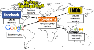
Figure 1: Use case: Movielens.

III Definitions and Background

In this section, we introduce the data model we use, and a CF algorithm based on matrix factorization. Then, we describe the recommendation problem we study.

III-A Data Model

We use matrices to represent all the data manipulated in our recommendation algorithm. Matrices are very useful mathematical structures to represent numbers, and several techniques from matrix theory and linear algebra can be used to analyze them in various contexts. Hence, we assume that any data source can be represented using a matrix, whose value in the $i,j$ position is a correlation that may exist between the $i^{th}$ and $j^{th}$ elements. We distinguish mainly three different kinds of data matrices:

Users’ preferences history: In a recommender system, there are two classes of entities, which are referred as users and items. Users have preferences for certain items, and these preferences are extracted from the data. The data itself is represented as a matrix $R$, giving for each user-item pair, a value that represents the degree of preference of that user for that item.

Users’ attributes: A data source may supply information on users using two classes of entities, which are referred to users and attributes. An attribute may refer to any abstract entity that has a relation with users. We also use matrices to represent such data, where for each user-attribute pair, a value represents their correlation (e.g., term frequency-inverse document frequency (tf-idf) [11]). The way this correlation is computed is out of the scope of this paper.

Items’ attributes: Similarly, a data source may embed information that describes items using two classes of entities, namely items and attributes. Here, an attribute refers to any abstract entity that has a relation with items. Matrices are used to represent these data, where for each attribute-item pair, a value is associated to represent their correlation (e.g., tf-idf). The way this correlation is computed is also beyond the scope of this paper.

Table I gives examples of attributes that may describe both users and items, as well as the meaning of the correlations. It is interesting to notice that these three kinds of matrices are sparse matrices, meaning that most entries are missing. A missing value implies that we have no explicit information regarding the corresponding entry.

TABLE I: SAMPLE OF ATTRIBUTES.

Attribute 1	Attribute 2	Example of correlation
User	User	Similarity between the two users
User	Topic	Interest of the user in the topic
Item	Topic	Topic of the items
Item	Item	Similarity between two items

III-B Matrix Factorization (MF) Models

Matrix factorization aims at decomposing a user-item rating matrix $R$ of dimension $I\times J$ containing observed ratings $r_{i,j}$ into a product $R\approx U^{T}V$ of latent feature matrices U and V of rank K. In this initial MF setting, we designate $U_{i}$ and $V_{j}$ as the $i^{th}$ and $j^{th}$ columns of $U$ and $V$ such that $U_{i}^{T}V_{j}$ acts as a measure of similarity between user $i$ and item $j$ in their respective k-dimensional latent spaces $U_{i}$ and $V_{j}$.

However, there remains the question of how to learn $U$ and $V$ given that $R$ may be incomplete (i.e., it contains missing entries). One answer is to define a reconstruction objective error function over the observed entries, that are to be minimized as a function of $U$ and $V$, and then use gradient descent to optimize it; formally, we can optimize the following MF objective [12]: $\frac{1}{2}{\displaystyle\sum_{i=1}^{I}{\displaystyle\sum_{j=1}^{J}}I_{ij}^{R}(r_{ij}-U_{i}^{T}V_{j})^{2}}$, where $I_{ij}$ is the indicator function that is equal to 1 if user $u_{i}$ rated item $v_{j}$ and equal to 0 otherwise. Also, in order to avoid overfitting, two regularization terms are added to the previous equation (i.e., $\frac{1}{2}\|U\|_{F}^{2}$ and $\frac{1}{2}\|V\|_{F}^{2}$).

III-C Problem Definition

The problem we address in this paper is different from that in traditional recommender systems, which consider only the user-item rating matrix $R$. In this paper, we incorporate information coming from multiple and diverse data matrices to improve recommendation quality. We define the problem we study in this paper as follows. Given:

• a user-item rating matrix $R$;

• $N$ data matrices that describe the user preferences $\{S^{U^{1}},\ldots,S^{U^{n}}\}$ distributed over different clusters;

• $M$ data matrices that describe the items’ characteristics $\{S^{V^{1}},\ldots,S^{V^{m}}\}$ distributed over different clusters;

How to effectively and efficiently predict the missing values of the user-item matrix $R$ by exploiting and combining these different data matrices?

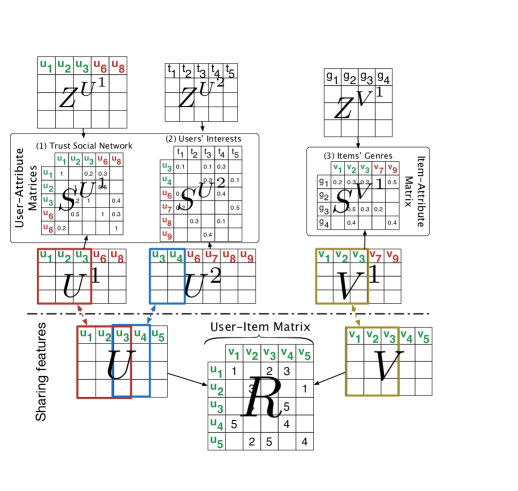
Figure 2: Overview of the recommendation model using toy data. Users and items in green are users for which we make the recommendation, whereas users and items in red are used as additional knowledge.

IV Recommendation Model

In this section, we first give an overview of our recommendation model using an example. Then, we introduce the factor analysis method for our model that uses probabilistic matrix factorization.

IV-A Recommendation Model Overview

Let us first consider as an example the user-item rating matrix $R$ of a recommender system (see Figure 2). There are 5 users (from $u_{1}$ to $u_{5}$) who rated 5 movies (from $v_{1}$ to $v_{5}$) on a 5-point integer scale to express the extent to which they like each item. Also, as illustrated in Figure 2, the recommender system provider holds three data matrices that provide information that describe users and items. Note that only part of the users and items of these data matrices overlap with those of the user-item rating matrix.

1. Matrix (1): provides the social network of $u_{1}$, $u_{2}$, and $u_{3}$, where each value in the matrix $S^{U^{1}}$ represents the trustiness between two users.

2. Matrix (2): provides information about the interests of $u_{3}$ and $u_{4}$, where for each user-topic pair in the matrix $S^{U^{2}}$, a value is associated, which represents the interest of the user in this topic.

3. Matrix (3): provides information about the genre of the movies $v_{1}$, $v_{2}$, and $v_{3}$ in the matrix $S^{V^{1}}$.

The problem we study in this paper is how to predict the missing values of the user-item matrix $R$ effectively and efficiently by combining all these data matrices ($S^{U^{1}}$, $S^{U^{2}}$, and $S^{V^{1}}$). Motivated by the intuition that more information will help to improve a recommender system, and inspired by the solution proposed in [1], we propose to disseminate the data matrices of the data sources in the user-item matrix, by factorizing all these matrices simultaneously and seamlessly as illustrated in Figure 2, such as: $R\thickapprox U^{T}V$, $S^{U^{1}}\thickapprox U^{1T}Z^{U^{1}}$, $S^{U^{2}}\thickapprox U^{2T}Z^{U^{2}}$, and $S^{V^{1}}\thickapprox Z^{V^{1}T}V^{1}$, where the k-dimensional matrices $U$, $U^{1}$, and $U^{2}$ denote the user latent feature space, such as $U_{1}=U_{1}^{1}$, $U_{2}=U_{2}^{1}$, $U_{3}=U_{3}^{1}=U_{1}^{2}$, $U_{4}=U_{2}^{2}$ ($U_{1}$, $U_{2}$, $U_{4}$, and $U_{4}$ refer respectively to the $1^{st}$, $2^{nd}$, $3^{rd}$, and $4^{th}$ column of the matrix $U$), the matrices $V$ and $V^{1}$ are the k-dimensional item latent feature space such as $V_{1}=V_{1}^{1}$, $V_{2}=V_{2}^{1}$, $V_{3}=V_{3}^{1}$, and $Z^{U^{1}}$, $Z^{U^{2}}$, and $Z^{V^{1}}$, are factor matrices. In the example given in Figure 2, we use 3 dimensions to perform the factorizations of the matrices. Once done, we can predict the missing values in the user-items matrix $R$ using $U^{T}V$. In the following sections, we present the details of our recommendation model.

IV-B User-Item Rating Matrix Factorization

Suppose that a Gaussian distribution gives the probability of an observed entry in the User-Item matrix as follows:

$$r_{ij}\sim\mathcal{N}(r_{ij}|U_{i}^{T}V_{j},\sigma_{R}^{2})$$ (1)

where $\mathcal{N}(x|\mu,\sigma^{2})$ is the probability density function of the Gaussian distribution with mean $\mu$ and variance $\sigma^{2}$. The idea is to give the highest probability to $r_{ij}\approx U_{i}^{T}V_{j}$ as given by the Gaussian distribution. Hence, the probability of observing approximately the entries of $R$ given the feature matrices $U$ and $V$ is:

$$p(R|U,V,\sigma_{R}^{2})={\displaystyle\prod_{i=1}^{I}}{\displaystyle\prod_{j=1}^{J}}\left[\mathcal{N}(r_{ij}|U_{i}^{T}V_{j},\sigma_{R}^{2})\right]^{I_{ij}^{R}}$$ (2)

where $I_{ij}^{R}$ is the indicator function that is equal to 1 if a user $i$ rated an item $j$ and equal to 0 otherwise. Similarly, we place zero-mean spherical Gaussian priors [13][1][12] on user rating and item feature vectors:

$$\begin{array}[]{c}p(U|\sigma_{U}^{2})={\displaystyle\prod_{i=1}^{I}}\left[\mathcal{N}(U_{i}|0,\sigma_{U}^{2})\right],p(V|\sigma_{V}^{2})={\displaystyle\prod_{j=1}^{J}}\left[\mathcal{N}(V_{j}|0,\sigma_{V}^{2})\right]\end{array}$$ (3)

Hence, through a simple Bayesian inference, we have:

$$\begin{array}[]{c}p(U,V|R,\sigma_{R}^{2},\sigma_{U}^{2},\sigma_{V}^{2})\propto p(R|U,V,\sigma_{R}^{2})p(U|\sigma_{U}^{2})p(V|\sigma_{V}^{2})\end{array}$$ (4)

IV-C Matrix factorization for data sources that describe users

Now let’s consider a User-Attribute matrix $S^{U^{n}}$ of $P$ users and $K$ attributes, which describes users. We define the conditional distribution over the observed matrix values as:

$$p(S^{U^{n}}|U^{n},Z^{U^{n}},\sigma_{S^{U^{n}}}^{2})={\displaystyle\prod_{p=1}^{P}}{\displaystyle\prod_{k=1}^{K}}\left[\mathcal{N}(s_{pk}^{U^{n}}|U_{p}^{nT}Z_{k}^{U^{n}},\sigma_{S^{U^{n}}}^{2})\right]^{I_{pk}^{S^{U^{n}}}}$$ (5)

where $I_{pk}^{S^{U^{n}}}$ is the indicator function that is equal to 1 if user $p$ has a correlation with attribute $k$ (in the data matrix $S^{U^{n}}$) and equal to 0 otherwise. Similarly, we place zero-mean spherical Gaussian priors on feature vectors:

$$\begin{array}[]{cc}p(U^{n}|\sigma_{U}^{2})={\displaystyle\prod_{p=1}^{P}}\left[\mathcal{N}(U_{p}^{n}|0,\sigma_{U}^{2})\right],&p(Z^{U^{n}}|\sigma_{Z^{U^{n}}}^{2})={\displaystyle\prod_{k=1}^{K}}\left[\mathcal{N}(Z_{k}^{U_{n}}|0,\sigma_{Z^{U^{n}}}^{2})\right]\end{array}$$ (6)

Hence, similar to Equation 4, through a simple Bayesian inference, we have:

$$\begin{array}[]{c}p(U^{n},Z^{U^{n}}|S^{U^{n}},\sigma_{S^{U^{n}}}^{2},\sigma_{U}^{2},\sigma_{Z^{U^{n}}}^{2})\propto\\ \vphantom{{\displaystyle\prod_{i=1}^{I}}}p(S^{U^{n}}|U^{n},Z^{U^{n}},\sigma_{S^{U^{n}}}^{2})p(U^{n}|\sigma_{U}^{2})p(Z^{U^{n}}|\sigma_{Z^{U^{n}}}^{2})\end{array}$$ (7)

IV-D Matrix factorization for data sources that describe items

Now let’s consider an Item-Attribute matrix $S^{V^{m}}$ of $H$ items and $K$ attributes, which describes items. We also define the conditional distribution over the observed matrix values as:

$$\begin{array}[]{l}p(S^{V^{m}}|V^{m},Z^{V^{m}},\sigma_{S^{V^{m}}}^{2})=\\ {\displaystyle\prod_{h=1}^{H}}{\displaystyle\prod_{k=1}^{K}}\left[\mathcal{N}(s_{hk}^{V^{m}}|V_{h}^{mT}Z_{k}^{V^{m}},\sigma_{S^{V^{m}}}^{2})\right]^{I_{hk}^{S^{V^{m}}}}\end{array}$$ (8)

where $I_{hk}^{S^{V^{m}}}$ is the indicator function that is equal to 1 if an item $h$ is correlated to an attribute $k$ (in the datasource $S^{V^{m}}$) and equal to 0 otherwise. We also place zero-mean spherical Gaussian priors on feature vectors:

$$\begin{array}[]{c}p(V^{m}|\sigma_{V}^{2})={\displaystyle\prod_{h=1}^{H}}\left[\mathcal{N}(V_{h}^{m}|0,\sigma_{V}^{2})\right]\\ p(Z^{V^{m}}|\sigma_{Z^{V^{m}}}^{2})={\displaystyle\prod_{k=1}^{K}}\left[\mathcal{N}(Z_{k}^{V^{m}}|0,\sigma_{Z^{V^{m}}}^{2})\right]\end{array}$$ (9)

Hence, through a Bayesian inference, we also have:

$$\begin{array}[]{c}p(V^{m},Z^{V^{m}}|S^{V^{m}},\sigma_{S^{V^{m}}}^{2},\sigma_{V}^{2},\sigma_{Z^{V^{m}}}^{2})\propto\\ \vphantom{{\displaystyle\prod_{i=1}^{I}}}p(S^{V^{m}}|V^{m},Z^{V^{m}},\sigma_{S^{V^{m}}}^{2})p(V^{m}|\sigma_{V}^{2})p(Z^{V^{m}}|\sigma_{Z^{V^{m}}}^{2})\end{array}$$ (10)

IV-E Recommendation Model

Considering $N$ data matrices that describe users, $M$ data matrices that describe items, and based on the graphical model given in Figure 3, we model the conditional distribution over the observed ratings as:

$$\begin{array}[]{l}p(U,V|R,S^{U^{1}},\ldots,S^{U^{n}},S^{V^{1}},\ldots,S^{V^{m}}\\ \sigma_{Z^{U^{1}}}^{2}\ldots,\sigma_{Z^{U^{n}}}^{2},\sigma_{Z^{V^{1}}}^{2},\ldots,\sigma_{Z^{V^{m}}}^{2})\propto\\ p(R|U,V,\sigma_{R}^{2})p(U|\sigma_{U}^{2})p(V|\sigma_{V}^{2})\\ {\displaystyle\prod_{n=1}^{N}p(S^{U^{n}}|U^{n},Z^{U^{n}},\sigma_{S^{U^{n}}}^{2})p(U^{n}|\sigma_{U}^{2})p(Z^{U^{n}}|\sigma_{Z^{U^{n}}}^{2})}\\ {\displaystyle\prod_{m=1}^{M}p(S^{V^{m}}|V^{m},Z^{V^{m}},\sigma_{S^{V^{m}}}^{2})p(V^{m}|\sigma_{V}^{2})p(Z^{V^{m}}|\sigma_{Z^{V^{m}}}^{2})}\end{array}$$ (11)

Hence, we can infer the log of the posterior distribution for the recommendation model as follows:

$${\normalcolor\begin{array}[]{l}\mathcal{L}(U,U^{1},\ldots,U^{n},V,V^{1},\ldots,V^{m},Z^{U_{1}},\ldots,Z^{U_{n}},Z^{V_{1}},\ldots,Z^{V_{m}})=\\ \left.\frac{1}{2}{\displaystyle\sum_{i=1}^{I}{\displaystyle\sum_{j=1}^{J}}I_{ij}^{R}(r_{ij}-U_{i}^{T}V_{j})^{2}}\right\}\begin{array}[]{l}\textrm{Error over the }\\ \textrm{reconstruction of }R\end{array}\\ \left.+{\displaystyle\sum_{n=1}^{N}\frac{\lambda_{S^{U^{n}}}}{2}{\displaystyle\sum_{p=1}^{P}{\displaystyle\sum_{k=1}^{K}}I_{pk}^{S^{U^{n}}}(s_{pk}^{U^{n}}-U_{p}^{nT}Z_{k}^{U^{n}})^{2}}}\right\}\begin{array}[]{l}\textrm{Error over the}\\ \textrm{reconstruction of}\\ \textrm{datasources that }\\ \textrm{describe users}\end{array}\\ \left.+{\displaystyle\sum_{m=1}^{M}\frac{\lambda_{S^{V^{m}}}}{2}{\displaystyle\sum_{h=1}^{H}{\displaystyle\sum_{k=1}^{K}}I_{hk}^{S^{V^{m}}}(s_{hk}^{V^{m}}-V_{h}^{mT}Z_{k}^{V^{m}})^{2}}}\right\}\begin{array}[]{l}\textrm{Error over the}\\ \textrm{reconstruction of}\\ \textrm{datasources that }\\ \textrm{describe items}\end{array}\\ \left.\begin{array}[]{l}+\frac{\lambda_{U}}{2}(\|U\|_{F}^{2}+{\displaystyle\sum_{n=1}^{N}\|U^{n}\|_{F}^{2}})\\ +\frac{\lambda_{V}}{2}(\|V\|_{F}^{2}+{\displaystyle\sum_{m=1}^{M}\|V^{m}\|_{F}^{2}})\\ +{\displaystyle\sum_{n=1}^{N}\frac{\lambda_{Z^{U^{n}}}}{2}\|Z^{U^{n}}\|_{F}^{2}}+{\displaystyle\sum_{m=1}^{M}\frac{\lambda_{Z^{U^{m}}}}{2}\|Z^{U^{m}}\|_{F}^{2}}\end{array}\right\}\begin{array}[]{l}\textrm{Regularization}\\ \textrm{terms}\end{array}\end{array}}$$ (12)

where $\|.\|_{F}^{2}$ denotes the Frobenius norm, and $\lambda_{*}$ are regularization parameters. A local minimum of the objective function given by Equation 12 can be found using Gradient Descent (GD) as detailed in Algorithm 4. We present this algorithm in details in Appendix A and a distributed version of this algorithm in the next section.

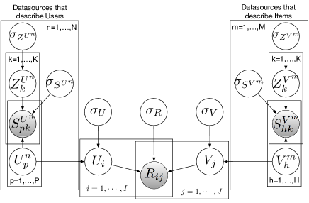
Figure 3: Graphical model for recommendation.

V Distributed Recommendation

In this section, we first present a distributed version of the Collaborative Filtering Algorithm 4, which minimizes Equation 12, and then we carry out a complexity analysis to show that it can scale to large datasets.

V-A Distributed CF Algorithm

input : The User-Item matrix $R_{ij}$;

A learning parameter $\alpha$;

Regularization parameters $\lambda_{U}$, $\lambda_{V}$;

output : Feature matrices $U$, $V$;

1

2

3Initialize latent feature matrices to small random values.

4

/* Minimize $\mathcal{L}$ using gradient descent as follows: */

5

while $\mathcal{L}>\epsilon$ /* $\epsilon$ is a stop criterion */

6 do

7      

      /* Compute local intermediate results of the gradient of $U$ as follows: */

8      

9      $\nabla_{U}=\left({\displaystyle I^{R}(U^{T}V-R)V}^{T}\right)^{T}+\lambda_{U}U$

10      

11      foreach  user $u_{i}$  do

12            

13            

14            Send $U_{i}$ to data sources that share information about the user $u_{i}$

15            

16       end foreach

17      

18      foreach  $\pi_{n}$ received  do

19            

20            

            /* $\oplus$ is an algebraic operator given in Definition 1. */

21            

22            $\nabla_{U}=\nabla_{U}\oplus\pi_{n}$

23            

24       end foreach

25      

      /* Compute local intermediate results of the gradient of $V$ as follows: */

26      

27      $\nabla_{V}=\left({\displaystyle I^{R}(U^{T}V-R)^{T}U^{T}}\right)^{T}+\lambda_{V}V$

28      

29      foreach  item $v_{j}$  do

30            

31            Send $V_{j}$ to data sources that share information about the item $v_{j}$

32       end foreach

33      

34      foreach  $\pi_{m}$ received  do

35            

36            $\nabla_{V}=\nabla_{V}\oplus\pi_{m}$

37            

38       end foreach

39      

      /* Update global $U$ and $V$ latent features matrices as follows: */

40      

41      $U=U-\alpha\left(\nabla_{U}\right)$

42      

43      $V=V-\alpha\left(\nabla_{V}\right)$

44      

45      check $U$ and $V$ for convergence

46      

47 end while

48

Algorithm 1 Distributed Collaborative Filtering Algorithm (Master Cluster 1/3)

1

2

3Initialize latent feature matrices $Z^{U^{n}}$ and $U^{n}$ to small random values.

4 Procedure RefineUserFeatures()

5      

       input : A User-Object matrix $S^{U_{n}}$;

       The common user latent features matrix $U$;

       A learning parameter $\alpha$;

       Regularization parameters $\lambda_{S^{U_{n}}},\lambda_{Z^{U_{n}}}$;

6      

7      foreach  $U_{i}$ received  do

8            

9            

10            Replace the right latent user feature vector $U_{k}^{n}$ with the received $U_{i}$

11            

12       end foreach

13      

      /* Compute intermediate result: */

14      

15      $\pi_{n}=\lambda_{S^{U^{n}}}\left({\displaystyle I^{S^{U^{n}}}(U^{nT}Z^{U^{n}}-S^{U^{n}})Z^{U^{n}}{}^{T}}\right)^{T}$

16      

17      Keep in $\pi_{n}$ vectors of users that are shared with the recommender system

18      

19      Send $\pi_{n}$ to the recommender system

20      

      /* Compute gradients of $U^{n}$ and $Z$ with respect to $\mathcal{L}$ */

21      

22      $\nabla_{U^{n}}=\lambda_{S^{U^{n}}}\left({\displaystyle I^{S^{U^{n}}}(U^{nT}Z^{U^{n}}-S^{U^{n}})Z^{U^{n}}{}^{T}}\right)^{T}+\lambda_{S^{U^{n}}}U^{n}$

23      

24      

25      $\nabla_{Z}=\left(\lambda_{S^{U^{n}}}{\displaystyle\left(I^{S^{U^{n}}}(U^{nT}Z^{U^{n}}-S^{U^{n}})\right)^{T}U^{nT}}\right)^{T}+\lambda_{Z^{U^{n}}}Z^{U^{n}}$

26      

      /* Update local latent features matrices $U$ and $Z$ as follows: */

27      

28      $U^{n}=U^{n}-\alpha\left(\nabla_{U^{n}}\right)$

29      $Z^{U^{n}}=Z^{U^{n}}-\alpha\left(\nabla_{Z}\right)$

30      

31

Algorithm 2 Distributed Collaborative Filtering Algorithm (User data slave cluster 2/3)

1

2

3Initialize latent feature matrices $Z^{V^{m}}$ and $V^{m}$ to small random values.

4 Procedure RefineUserFeatures()

       input : An Object-Item matrix $S^{V_{m}}$;

       The common user latent features matrix $V$;

       A learning parameter $\alpha$;

       Regularization parameters $\lambda_{S^{V_{m}}},\lambda_{Z^{V_{m}}}$;

5      

6      foreach  $V_{j}$ received  do

7            

8            Replace the right latent item feature vector $V_{k}^{m}$ with the received $V_{j}$

9       end foreach

10      

      /* Compute intermediate result: */

11      

12      $\pi_{m}=\lambda_{S^{V^{m}}}\left({\displaystyle\left(I^{S^{V^{m}}}(Z^{V^{m}T}V^{m}-S^{V^{m}})\right)^{T}Z^{V^{m}}{}^{T}}\right)^{T}$

13      Keep in $\pi_{m}$ vectors of items that are shared with the recommender system

14      Send $\pi_{m}$ to the recommender system

      /* Compute gradients of $V$ and $Z$ with respect to $\mathcal{L}$: */

15      

16      $\nabla_{V^{m}}=\lambda_{S^{V^{m}}}\left({\displaystyle\left(I^{S^{V_{m}}}(Z^{V^{m}T}V^{m}-S^{V^{m}})\right)^{T}Z^{V^{m}}{}^{T}}\right)^{T}+\lambda_{S^{V^{m}}}V^{m}$

17      

18      $\nabla_{Z}=\lambda_{S^{V^{m}}}\left({\displaystyle I^{S^{V^{m}}}(Z^{V^{m}T}V^{m}-S^{V^{m}})V^{T}}\right)^{T}+\lambda_{Z^{U^{m}}}Z$

19      

      /* Update local latent features matrices $V$ and $Z$ as follows: */

20      

21      $V^{m}=V^{m}-\alpha\left(\nabla_{V^{m}}\right)$

22      $Z^{V^{m}}=Z^{V^{m}}-\alpha\left(\nabla_{Z}\right)$

23

Algorithm 3 Distributed Collaborative Filtering Algorithm (Item data slave cluster 3/3)

In this section we show how to deploy Algorithm 4 in a distributed setting over different clusters and how to generate predictions. This distribution is mainly motivated by: (i) the need to scale up our collaborative filtering algorithm to very large datasets, i.e., parallelize part of the computation, and (ii) avoid to transfer the raw data matrices (for mainly privacy concerns). Instead, we only exchange common latent features.

Based on the observation that several parts of the centralized CF algorithm (see Algorithm 4) can be executed in parallel and separately on different clusters, we propose to distribute it using Algorithms 1, 2, and 3. Algorithm 1 is executed by the master cluster that handle the user-item rating matrix, whereas each slave cluster that handles data matrices about users’ attributes executes an instance of Algorithm 2, and each slave cluster that hanldes data matrices about items’ attributes executes an instance of Algorithm 3.

Basically, the first step of this distributed algorithm is an initialization phase, where each cluster (master and slaves) initializes its latent feature matrices with small random values (lines 1 of Algorithms 1, 2, and 3). Next, in line 1 of Algorithm 1, the master cluster computes part of the partial derivative of the objective function given in Equation 12 with respect to $U$ (line 1 of Algorithm 1 computes a part of line 4 in Algorithm 4). Then, for each user $u_{i}$, the master cluster sends its latent feature vector to the other participant slave clusters, which share attributes about that user (lines 1 and 1 in Algorithm 1). Then, the master cluster waits for responses of all these participant slave clusters (line 1 in Algorithm 1).

Next, each slave cluster that receives users’ latent features replaces the corresponding user latent feature vector $U_{k}^{n}$ with the user latent feature vector $U_{i}$ received from the master cluster (lines 2 and 2 in Algorithm 2). Then, the slave cluster computes $\pi_{n}$, which is part of the partial derivative of the objective function given in Equation 12 with respect to $U$ (line 2 in Algorithm 2 computes a part of line 4 in Algorithm 4). Next, the slave cluster keeps in $\pi_{n}$, only vectors of users that are shared with the master cluster (line 2 in Algorithm 2). The slave cluster sends the remaining feature vectors in $\pi_{n}$ to the master cluster (line 2 in Algorithm 2). Finally, the slave cluster updates its local user and attribute latent feature matrices $Z^{U^{n}}$ and $U^{n}$ (lines 9-2 in Algorithm 2).

As for the master cluster, each user latent feature matrix $\pi_{n}$ received from a slave cluster is added to $\nabla_{U}$, which is the partial derivative of the objective function with respect to $U$ (line 1 in Algorithm 1). This addition is performed using $\oplus$, an algebraic operator defined as follows:

Definition 1.

For two matrices $A_{m,n}=(a_{ij})$ and $B_{m,p}=(b_{ij})$, $A\oplus B$ returns the matrix $C_{m,n}$ where:

$$c_{ij}=\left\{\begin{array}[]{ll}a_{ij}+b_{ij}&\textrm{if }A_{j}=B_{j}\begin{array}[]{c}\textrm{(the column refers}\\ \textrm{ to the same user/item)}\end{array}\\ a_{ij}&\textrm{otherwise}\end{array}\right.$$

Once the master cluster has received all the partial derivative of the objective function with respect to $U$ from all the user participant sites, it has computed the global derivative of the objective function given in Equation 12 with respect to $U$ . A similar operation is performed for item slave cluster from line 1 to line 1 in Algorithm 1 to compute the global derivative of the objective function given in Equation 12 with respect to $V$ as given in line 4 of Algorithm 4. Finally, the master cluster updates the user and item latent feature matrices $U$ and $V$, and evaluates $\mathcal{L}$ in lines 1, 1, and 1 of Algorithm 1 respectively. The convergence of the whole algorithm is checked in line 1 of Algorithm 1. Note that all the involved clusters that hold data matrices on users and items’ attributes execute their respective algorithm in parallel.

V-B Complexity Analysis

The main computation of the GD algorithm evaluates the objective function $\mathcal{L}$ in Equation 12 and its derivatives. Because of the extreme sparsity of the matrices, the computational complexity of evaluating the object function $\mathcal{L}$ is $O(\rho_{1}+\ldots+p_{n})$, where $\rho_{n}$ is the number of nonzero entries in matrix $n$. The computational complexities for the derivatives are also proportional to the number of nonzero entries in data matrices. Hence, the total computational complexity in one iteration of this gradient descent algorithm is $O(\rho_{1}+\ldots+p_{n})$, which indicates that the computational time is linear with respect to the number of observations in the data matrices. This complexity analysis shows that our algorithm is quite efficient and can scale to very large datasets.

VI Experimental Evaluation

In this section, we carry out several experiments to mainly address the following questions:

1. What is the amount of data transferred?

2. How does the number of user and item sources affect the accuracy of predictions?

3. What is the performance comparison on users with different observed ratings?

4. Can our algorithm achieve good performance even if users have no observed ratings?

5. How does our approach compare with the state-of-the-art collaborative filtering algorithms?

In the rest of this section, we introduce our datasets and experimental methodology, and address these questions (question 1 in Section VI-C, question 2 in Section VI-D, questions 3 and 4 in Section VI-E, and question 5 in Section VI-F).

VI-A Description of the Datasets

The first round of our experiment is based on a dataset from Delicious, described and analyzed in [14][15][16] (http://data.dai-labor.de/corpus/delicious/). Delicious is a bookmarking system, which provides to the user a means to freely annotate Web pages with tags. Basically, in this scenario we want to recommend interesting Web pages to users. This dataset contains 425,183 tags, 1,321,039 Web pages, and 318,769 users. The user-item matrix contains 2,265,207 entries (a density of $\simeq 0.0005\%$). Each entry of the user-item matrix represents the degree of which a user interacted with an item expressed on a $[0,1]$ scale. The dataset contains a user-tag matrix with 4,598,815 entries, where each entry expresses the interest of a user in a tag on a $[0,1]$ scale. Lastly, the dataset contains an item-tags matrix with 4,403,244 entries, where each entry expresses the coverage of a tag in a Web page on a $[0,1]$ scale. The user-tag matrix and item-tags are used as user data matrix, and item data matrix respectively. However, to simulate having many data matrices that describe both users and items, we have manually and randomly broken the two previous matrices into 10 matrices in both columns and rows. These new matrices kept their property of sparsity. Hence, we end up with a user-item rating matrix, 10 user data matrices (with approximately 459 000 entries each), and 10 item data matrices (with approximately 440 000 entries each).

The second round of experiments is based on one of the datasets given by the HetRec 2011 workshop (http://ir.ii.uam.es/hetrec2011/datasets.html), and reflect a real use case. This dataset is an extension of the Movielens dataset, which contains personal ratings, and data coming from other data sources (mainly IMDb and Rotten Tomatoes). This dataset includes ratings that range from 1 to 5, including 0.5 steps. This dataset contains a user-items matrix of 2,113 users, 10,109 movies, and 855,597 ratings (with a density of $\simeq 4\%$). This dataset also includes a user-tag matrix of 9,078 tags describing the users with 21,324 entries on a $[0,1]$ scale, which is used as a user data matrix. Lastly, this dataset contains four item data matrices: (1) an item-tag matrix with 51,794 entries, (2) an item-genre matrix with 20 genres and 20,809 entries, (3) an item-actor matrix with 95,321 actors, and 213,742 entries, and (4) an item-location matrix with 187 locations and 13,566 entries.

VI-B Methodology and metrics

We have implemented our distributed collaborative algorithm and integrated it into Peersim [17], a well-known distributed computing simulator. We use two different training data settings (80% and 60%) to test the algorithms. We randomly select part of the ratings from the user-item rating matrix as the training data (80% or 60%) to predict the remaining ratings (respectively 20% or 40%). The random selection was carried out 5 times independently, and we report the average results. To measure the prediction quality of the different recommendation methods, we use the Root Mean Square Error (RMSE), for which a smaller value means a better performance. We refer to our method Distributed Probabilistic Matrix Factorization (DPMF).

VI-C Data transfer

Let’s consider an example where a recommender system uses a social network as a source of information to improve its precision. Let’s assume that the social network contains 40 million unique users with 80 billion asymmetric connections (a density of $0.005\%$). It turns out that if we only consider the connections, the size of the user-user matrix representing this social network is $80\times 10^{9}\times(8\,B+8\,B)\simeq 1.16\,TB$ (assuming that we need 8 bytes to encode a double to represent the strength of the relation between two users, and 8 bytes to encode a long that represents the key for the entry of the value in the user-user matrix). Hence, for the execution of the centralized collaborative filtering algorithm, $1.16\,TB$ of data need to be transferred through the network. However, if we assume that there are 10% of common users between the recommender system and the social network, each iteration of the DPMF algorithm requires the transfer of $4\times 10^{6}\times 10\times 8\,B\times 2\simeq 610\,MB$ (assuming that we use 10 dimensions for the factorization, that we need 8 bytes to encode a double value in a latent user vector, and a round trip of transfer for the latent vectors in line 1 of Algorithm 1 and line 2 of Algorithm 2). Hence, if the algorithm requires 100 iterations to converge (roughly the number of iterations needed in our experiment), the total amount of data transferred is $59\,GB$, which represents $5\%$ of the data transferred in the centralized solution. Finally, the total amount of data transferred depends on the density of the source, the total number of common attributes, the number of latent dimensions used for the factorization and the number of iterations needed for the algorithm to converge. These parameters can make the DPMF very competitive compared to the centralized solution in terms of data transfer.

(a) Training: 80%.

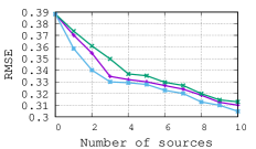
(b) Training: 60%.

Figure 4: Results of the impact of the number of sources on the Delicious dataset.

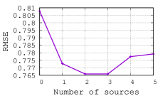
(a) Training: 80%.

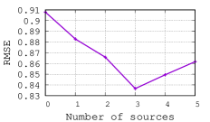
(b) Training: 60%.

Figure 5: Results of the impact of the number of sources on the Movielens dataset. The data matrices are added in the following order: (1) user-tag, (2) item-tag, (3) item-genre, (4) item-actor, and (5) item-location.

VI-D Impact of the number of sources

Figures 4 and 5 show the results obtained on the two datasets, while varying the number of sources. Note that source=0 means that we factorize only the user-item matrix.

In Figure 4, the green curve represents the impact of adding item sources only, the red curve the impact of adding user sources only, and the blue curve the impact of adding both sources (e.g., 2 sources means we add 2 item and 2 user sources). First, the results show that adding more sources helps to improve the performance, confirming our initial intuition. The additional data sources have certainly contributed to refine users’ preferences and items’ characteristics. Second, we observe that sources that describe users are more helpful than sources that describe items (about 10% gain). However, we consider this observation to be specific to this dataset, and cannot be generalized. Third, we notice that combining both data sources provides the best performance (blue curve, about 8% with respect to the use of only user sources). Lastly, the best gain obtained with respect to the PMF method (source=0) is about 32%.

Figure 5 shows the results obtained on the Movielens dataset. The obtained results here are quite different than those obtained on the Delicious dataset. Indeed, we observe that the data matrices 1, 2 and 3 have a positive impact on the results; however, data matrices 4 and 5 decrease the performance. This is certainly due to the fact that the data embedded in these two matrices are not meaningful to extract and infer items’ characteristics. In general, the best performance is obtained using the three first data matrices, with a gain of 10% with respect to PMF (source=0).

VI-E Performance on users and items with different ratings

We stated previously that the data sparsity in a recommender system induces mainly two problems: (1) the lack of data to effectively model user preferences, and (2) the lack of data to effectively model item characteristics. Hence, in this section we study the ability of our method to provide accurate recommendations for users that supply few ratings, and items that contain few ratings (or no ratings at all). We show the results for different user ratings in Figure 6a, and for different item ratings in Figure 6b on the Delicious dataset. We group them into 10 classes based on the number of observed ratings: “0”, “1-5”, “6-10”, “11-20”, “21-40”, “41-80”, “81-160”, “161-320”, “321-640”, and “>640”. We show the results for different user ratings in Figure 6a, and for different item ratings in Figure 6b on the Delicious dataset. We also show the performance of the Probabilistic Matrix Factorization (PMF) method [12], and our method using 5 and 10 data matrices. In Figure 6a, on the X axis, users are grouped and ordered with respect to the number of ratings they have assigned. For example, for users with no ratings (0 on the X-axis), we got an average of 0.37 for RMSE using the PMF method. Similarly, in Figure 6b, on the X-axis, items are grouped and ordered with respect to the number of ratings they have obtained.

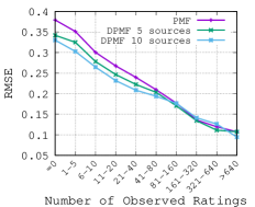
(a) Different users.

(b) Different items.

Figure 6: Performance for different ratings on the Delicious dataset.

TABLE II: PERFORMANCE COMPARISON USING RMSE. OPTIMAL VALUES OF THE PARAMETERS ARES USED FOR EACH METHOD (K= 10).

Dataset	Training	U. Mean	I. Mean	NMF	PMF	SoRec	PTBR	Matchbox	HeteroMF	DPMF
Delicious	80%	0.4389	0.4280	0.3814	0.3811	0.3566	0.3499	0.3297	0.3301	0.2939
		33,03%	31,33%	22,94%	22,88%	17.58%	16.00%	10.85%	10.96%	Improvement
	60%	0.3965	0.4087	0.3779	0.3911	0.3681	0.3599	0.3387	0.3434	0.3047
		23,15%	25,44%	19,37%	22,09%	17.22%	15.33%	10.03%	11.26%	Improvement
Movielens	80%	0.8399	0.8467	0.7989	0.8106	0.774	0.7801	0.7605	0.7788	0.7658
		8,82%	9,55%	4,14%	5,52%	1.05%	1.83%	-0.69%	1.66%	Improvement
	60%	0.9478	0.9667	0.9011	0.9096	0.882	0.8912	0.8399	0.8360	0.8365
		11,74%	13,46%	7,16%	8,03%	5.15%	6.13%	0.40%	-0.05%	Improvement

The results show that our method is more efficient in providing accurate recommendations compared to the PMF method for both users and items with few ratings (from 0 to about 100 on the-X axis). Also, the experiments show that the more we add data matrices, the more the recommendations are accurate. However, for clarity, we just plot the results obtained for our method while using 5 and 10 data matrices. Finally, we also noticed that the performance is better for predicting ratings to items that contain few ratings, than to users who rated few items. This is certainly due to the fact that users’ preferences change over time, and thus, the error margin is increased.

VI-F Performance comparison

To demonstrate the performance behavior of our algorithm, we compared it with eight other state-of-the-art algorithms: User Mean: uses the mean value of every user; Item Mean: utilizes the mean value of every item; NMF [18]; PMF [12], SoRec [1]; PTBR [19]; MatchBox [20]; HeteroMF [21]. The results of the comparison are shown in Table II. The optimal parameters of each method are selected, and we report the final performance on the test set. The percentages in Table II are the improvement rates of our method over the corresponding approaches.

First, from the results, we see that our method consistently outperforms almost all the other approaches in all the settings of both datasets. Our method can almost always generate better predictions than the state-of-the-art recommendation algorithms. Second, only Matchbox and HeteroMF slightly outperform our method on the Movielens dataset. Third, the RMSE values generated by all the methods on the Delicious dataset are lower than those on Movielens dataset. This is due to the fact that the rating scale is different between the two datasets. Fourth, our method outperforms the other methods better on the Delicious dataset, than on the Movielens dataset (10% to 33% on Delicious and -0.05% to 11% on Movielens). This is certainly due to the fact that: (1) the Movilens dataset contains less data (fewer users and fewer items), (2) there are less data matrices in the Movielens dataset to add, and (3) the data matrices of the Delicious dataset are of higher quality. Lastly, even if we use several data matrices in our method, using 80% of training data still provides more accurate predictions than 60% of training data. We explain this by the fact that the data of the user-item matrix are the main resources to train an effective recommendation model. Clearly, an external source of data cannot replace the user-item rating matrix, but can be used to enhance it.

VII Related work

Enhanced recommendation: Many researchers have started exploring social relations to improve recommender systems (including implicit social information, which can be employed to improve traditional recommendation methods [22]), essentially to tackle the cold-start problem [23][1][10]. However, as pointed in [24], only a small subset of user interactions and activities are actually useful for social recommendation.

In collaborative filtering based approaches, Liu and Lee [25] proposed very simple heuristics to increase recommendation effectiveness by combining social networks information. Guy et al. [26] proposed a ranking function of items based on social relationships. This ranking function has been further improved in [19] to include social content such as related terms to the user. More recently, Wang et al. [27] proposed a novel method for interactive social recommendation, which not only simultaneously explores user preferences and exploits the effectiveness of personalization in an interactive way, but also adaptively learns different weights for different friends. Also, Xiao et al. [28] proposed a novel user preference model for recommender systems that considers the visibility of both items and social relationships.

In the context of matrix factorization, following the intuition that a person’s social network will affect her behaviors on the Web, Ma et al. [1] propose to factorize both the users’ social network and the rating records matrices. The main idea is to fuse the user-item matrix with the users’ social trust networks by sharing a common latent low-dimensional user feature matrix. This approach has been improved in [29] by taking into account only trusted friends for recommendation while sharing the user latent dimensional matrix. Almost a similar approach has been proposed in [30] and [31] who include in the factorization process, trust propagation and trust propagation with inferred circles of friends in social networks respectively. In this same context, other approaches have been proposed to consider social regularization terms while factorizing the rating matrix. The idea is to handle friends with dissimilar tastes differently in order to represent the taste diversity of each user’s friends [2][3]. A number of these methods are reviewed, analyzed and compared in [32].

Also, few works consider cross-domain recommendation, where a user’s acquired knowledge in a particular domain could be transferred and exploited in several other domains, or offering joint, personalized recommendations of items in multiple domains, e.g., suggesting not only a particular movie, but also music CDs, books or video games somehow related with that movie. Based on the type of relations between the domains, Fernández-Tobías et al. [33] propose to categorize cross-domain recommendation as: (i) content based-relations (common items between domains) [34], and (ii) collaborative filtering-based relations (common users between domain) [35][36]. However, almost all these algorithms are not distributed.

Distributed recommendation: Serveral decentralized recommendation solutions have been proposed mainly from a peer to peer perspective, basically for collaborative filtering [37], search and recommendation [38]. The goal of these solutions is to decentralize the recommendation process.

Other works have investigated distributed recommendation algorithms to tackle the problem of scalability. Hence, Liu et al. [25] provide a multiplicative-update method. This approach is also applied to squared loss and to nonnegative matrix factorization with an “exponential” loss function. Each of these algorithms in essence takes an embarrassingly parallel matrix factorization algorithm developed previously and directly distributes it across a MapReduce cluster. Gemulla et al. [39] provide a novel algorithm to approximately factor large matrices with millions of rows, millions of columns, and billions of nonzero elements. The approach depends on a variant of the Stochastic Gradient Descent (SGD), an iterative stochastic optimization algorithm. Gupta et al. [40] describe scalable parallel algorithms for sparse matrix factorization, analyze their performance and scalability. Finally, Yu et al. [41] uses coordinate descent, a classical optimization approach, for a parallel scalable implementation of matrix factorization for recommender system. More recently, Shin et al. [42] proposed two distributed tensor factorization methods, CDTF and SALS. Both methods are scalable with all aspects of data and show a trade-off between convergence speed and memory requirements.

However, note that almost all the works described above focus mainly on decentralizing and parallelizing the matrix factorization computation. To the best of our knowledge, none of the existing distributed solutions proposes a distributed recommendation approach using diverse data sources.

VIII Conclusion

In this paper, we proposed a new distributed collaborative filtering algorithm, which uses and combines multiple and diverse data matrices provided by online services to improve recommendation quality. Our algorithm is based on the factorization of matrices, and the sharing of common latent features with the recommender system. This algorithm has been designed for a distributed setting, where the objective was to avoid sending the raw data, and parallelize the matrix computation. All the algorithms presented have been evaluated using two different datasets of Delicious and Movielens. The results show the effectiveness of our approach. Our method consistently outperforms almost all the state-of-the-art approaches in all the settings of both datasets. Only Matchbox and HeteroMF slightly outperform our method on the Movielens dataset.

input : The User-Item matrix $R_{ij}$; Matrices of datasources that describe users: $S_{ik}^{U^{1}},\cdots,S_{ik}^{U^{n}}$;

Matrices of datasources that describe items: $S_{ik}^{V^{1}},\cdots,S_{ik}^{V^{m}}$;

output : Feature matrices $U$, $V$

1

2

3Initialize feature vectors $U,V,Z^{U^{1}},\ldots,Z^{U^{n}},Z^{V^{1}},\ldots,Z^{V^{m}}$ to small random values.

/* Minimize $\mathcal{L}(U,V,Z^{U^{1}},\ldots,Z^{U^{n}},Z^{V^{1}},\ldots,Z^{V^{m}})$ using gradient descent as follows: */

4

while $\mathcal{L}(U,V,Z^{U^{1}},\ldots,Z^{U^{n}},Z^{V^{1}},\ldots,Z^{V^{m}})>\epsilon$/* $\epsilon$ is a stop criteria */

5 do

6      

      /* Update common Users’ Latent Features. */

7      

8      $U=\overbrace{{\displaystyle U-\alpha\left({\displaystyle I^{R}(U^{T}V-R)V}\oplus\overbrace{\lambda_{S^{U_{1}}}I^{S^{U^{1}}}(U^{1T}Z^{U^{1}}-S^{U^{1}})Z^{U^{1}}}^{\sslash\textrm{Performed by Algorithm \ref{alg:DistGradientDescent2}}}\oplus\cdots\oplus\overbrace{\lambda_{S^{U^{n}}}{\displaystyle I^{S^{U^{n}}}(U^{nT}Z^{U^{n}}-S^{U^{n}})Z^{U^{n}}}}^{\sslash\textrm{Performed by Algorithm \ref{alg:DistGradientDescent2}}}+\lambda_{U}U\right)}}^{\textrm{Performed by Algorithm \ref{alg:DistGradientDescent1}}}$

9      

      /* Update common Items’ Latent Features. */

10      

11      $V=\overbrace{V-\alpha\left({\displaystyle I^{R}(U^{T}V-R)U}\oplus\overbrace{\lambda_{S^{V^{1}}}{\displaystyle I^{S^{V^{1}}}(Z^{V^{1}T}V^{m}-S^{V^{1}})Z^{V^{1}}}}^{\sslash\textrm{Performed by Algorithm \ref{alg:DistGradientDescent3}}}\oplus\cdots\oplus\overbrace{\lambda_{S^{V^{m}}}{\displaystyle I^{S^{V^{m}}}(Z^{V^{m}T}V^{m}-S^{V^{m}})Z^{V^{m}}}}^{\sslash\textrm{Performed by Algorithm \ref{alg:DistGradientDescent3}}}+\lambda_{V}V\right)}^{\textrm{Performed by Algorithm \ref{alg:DistGradientDescent1}}}$

12      

      $\left.\begin{array}[]{l}\sslash\left\{U^{1}=U^{1}-\alpha\left(\lambda_{S^{U_{1}}}{\displaystyle I^{S^{U^{1}}}(U^{1T}Z^{U^{1}}-S^{U^{1}})Z^{U^{1}}}+\lambda_{S^{U^{1}}}U^{1}\right)\right.\\ \vdots\\ \sslash\left\{U^{n}=U^{n}-\alpha\left(\lambda_{S^{U^{n}}}{\displaystyle I^{S^{U^{n}}}(U^{nT}Z^{U^{n}}-S^{U^{n}})Z^{U^{n}}}+\lambda_{S^{U^{n}}}U^{n}\right)\right.\end{array}\right\}$/*

Update Non common Users’ Latent

Features performed by Algorithm 2

*/

13      

      $\left.\begin{array}[]{l}\sslash\left\{V^{1}=V^{1}-\alpha\left(\lambda_{S^{V_{1}}}{\displaystyle I^{S^{V_{1}}}(Z^{V_{1}T}V^{1}-S^{V_{1}})Z^{V_{1}}}+\lambda_{S^{V_{1}}}V^{1}\right)\right.\\ \vdots\\ \sslash\left\{V^{m}=V^{m}-\alpha\left(\lambda_{S^{V^{m}}}{\displaystyle I^{S^{V^{m}}}(Z^{V^{m}T}V^{m}-S^{V^{m}})Z^{V^{m}}}+\lambda_{S^{V^{m}}}V^{m}\right)\right.\end{array}\right\}$/*

Update Non common Items’ Latent

Features performed by Algorithm 3

*/

14      

      $\left.\begin{array}[]{l}\sslash\left\{Z^{U^{1}}=Z^{U^{1}}-\alpha\left(\lambda_{S^{U^{1}}}{\displaystyle I^{S^{U^{1}}}(U^{1T}Z^{U^{1}}-S^{U^{1}})U^{1T}}+\lambda_{Z^{U^{1}}}Z\right)\right.\\ \vdots\\ \sslash\left\{Z^{U^{n}}=Z^{U^{n}}-\alpha\left(\lambda_{S^{U^{n}}}I^{S^{U^{n}}}(U^{nT}Z^{U^{n}}-S^{U^{n}})U^{nT}+\lambda_{Z^{U^{n}}}Z\right)\right.\end{array}\right\}$/*

Update Latent Features of Datasources

that describe users performed by Algorithm 2

*/

15      

      $\left.\begin{array}[]{l}\sslash\left\{Z^{V^{1}}=Z^{V^{1}}-\alpha\left(\lambda_{S^{V^{1}}}{\displaystyle I^{S^{V^{1}}}(Z^{V^{1}T}V^{1}-S^{V^{1}})V^{1}}+\lambda_{Z^{U^{1}}}Z\right)\right.\\ \vdots\\ \sslash\left\{Z^{V^{m}}=Z^{V^{m}}-\alpha\left(\lambda_{S^{V^{m}}}{\displaystyle I^{S^{V^{m}}}(Z^{V^{m}T}V^{m}-S^{V^{m}})V^{m}}+\lambda_{Z^{U^{m}}}Z\right)\right.\end{array}\right\}$/*

Update Latent Features of Datasources

that describe items performed by Algorithm 3

*/

16      

17 end while

18

/* $\sslash$ are parts that may be computed separately and in parallel with no dependency. */

19

Algorithm 4 Collaborative Filtering Algorithm

Appendix A GRADIENT-BASED OPTIMIZATION

We seek to optimize the sum of the objective function in Equation 12 and we use gradient descent for this purpose in Algorithm 4. $\sslash$ are parts that may be computed separately and in parallel with no dependency. These parts are computed by Algorithms 1, 2, and 3. $\oplus$ is the algebraic operator given in Definition 1.

References

- [1] Hao Ma, Haixuan Yang, Michael R. Lyu, and Irwin King. Sorec: Social recommendation using probabilistic matrix factorization. In Proceedings of the 17th ACM Conference on Information and Knowledge Management, CIKM ’08, pages 931–940, New York, NY, USA, 2008. ACM.
- [2] Hao Ma, Dengyong Zhou, Chao Liu, Michael R. Lyu, and Irwin King. Recommender systems with social regularization. In Proceedings of the Fourth ACM International Conference on Web Search and Data Mining, WSDM ’11, pages 287–296, New York, NY, USA, 2011. ACM.
- [3] Joseph Noel, Scott Sanner, Khoi-Nguyen Tran, Peter Christen, Lexing Xie, Edwin V. Bonilla, Ehsan Abbasnejad, and Nicolas Della Penna. New objective functions for social collaborative filtering. In Proceedings of the 21st International Conference on World Wide Web, WWW ’12, pages 859–868, New York, NY, USA, 2012. ACM.
- [4] J. J. Levandoski, M. Sarwat, A. Eldawy, and M. F. Mokbel. Lars: A location-aware recommender system. In 2012 IEEE 28th International Conference on Data Engineering, pages 450–461, April 2012.
- [5] Hao Wang, Manolis Terrovitis, and Nikos Mamoulis. Location recommendation in location-based social networks using user check-in data. In Proceedings of the 21st ACM SIGSPATIAL International Conference on Advances in Geographic Information Systems, SIGSPATIAL’13, pages 374–383, New York, NY, USA, 2013. ACM.
- [6] Sofiane Abbar, Sihem Amer-Yahia, Piotr Indyk, and Sepideh Mahabadi. Real-time recommendation of diverse related articles. In Proceedings of the 22Nd International Conference on World Wide Web, WWW ’13, pages 1–12, New York, NY, USA, 2013. ACM.
- [7] Cai-Nicolas Ziegler, Sean M. McNee, Joseph A. Konstan, and Georg Lausen. Improving recommendation lists through topic diversification. In Proceedings of the 14th International Conference on World Wide Web, WWW ’05, pages 22–32, New York, NY, USA, 2005. ACM.
- [8] Mi Zhang and Neil Hurley. Avoiding monotony: Improving the diversity of recommendation lists. In Proceedings of the 2008 ACM Conference on Recommender Systems, RecSys ’08, pages 123–130, New York, NY, USA, 2008. ACM.
- [9] Paul Resnick and Hal R Varian. Recommender Systems. Commun. ACM, 40(3):56–58, 1997.
- [10] Suvash Sedhain, Scott Sanner, Darius Braziunas, Lexing Xie, and Jordan Christensen. Social collaborative filtering for cold-start recommendations. In Proceedings of the 8th ACM Conference on Recommender Systems, RecSys ’14, pages 345–348, New York, NY, USA, 2014. ACM.
- [11] Ricardo A Baeza-Yates and Berthier Ribeiro-Neto. Modern Information Retrieval. Addison-Wesley Longman Publishing Co., Inc., 2 edition, 2010.
- [12] Ruslan Salakhutdinov and Andriy Mnih. Probabilistic matrix factorization. In Proceedings of the 20th International Conference on Neural Information Processing Systems, NIPS’07, pages 1257–1264, USA, 2007. Curran Associates Inc.
- [13] Delbert Dueck and Brendan J Frey. Probabilistic sparse matrix factorization. Technical report, 2004.
- [14] Robert Wetzker, Carsten Zimmermann, and Christian Bauckhage. Analyzing Social Bookmarking Systems: A del.icio.us Cookbook. In ECAI, 2008.
- [15] Mohamed Reda Bouadjenek, Hakim Hacid, and Mokrane Bouzeghoub. SoPRa: A New Social Personalized Ranking Function for Improving Web Search. In Proceedings of the 36th International ACM SIGIR Conference on Research and Development in Information Retrieval, SIGIR ’13, pages 861–864, New York, NY, USA, 2013. ACM.
- [16] Mohamed Reda Bouadjenek, Hakim Hacid, Mokrane Bouzeghoub, and Athena Vakali. Persador: Personalized social document representation for improving web search. Information Sciences, 369:614 – 633, 2016.
- [17] A. Montresor and M. Jelasity. Peersim: A scalable p2p simulator. In Peer-to-Peer Computing, 2009. P2P ’09. IEEE Ninth International Conference on, pages 99–100, Sept 2009.
- [18] Daniel D Lee and H Sebastian Seung. Learning the parts of objects by non-negative matrix factorization. Nature, 401(6755):788–791, 1999.
- [19] Ido Guy, Naama Zwerdling, Inbal Ronen, David Carmel, and Erel Uziel. Social media recommendation based on people and tags. In Proceedings of the 33rd International ACM SIGIR Conference on Research and Development in Information Retrieval, SIGIR ’10, pages 194–201, New York, NY, USA, 2010. ACM.
- [20] David H. Stern, Ralf Herbrich, and Thore Graepel. Matchbox: Large scale online bayesian recommendations. In Proceedings of the 18th International Conference on World Wide Web, WWW ’09, pages 111–120, New York, NY, USA, 2009. ACM.
- [21] Mohsen Jamali and Laks Lakshmanan. Heteromf: Recommendation in heterogeneous information networks using context dependent factor models. In Proceedings of the 22Nd International Conference on World Wide Web, WWW ’13, pages 643–654, New York, NY, USA, 2013. ACM.
- [22] Hao Ma. An Experimental Study on Implicit Social Recommendation. In SIGIR, 2013.
- [23] Jovian Lin, Kazunari Sugiyama, Min-Yen Kan, and Tat-Seng Chua. Addressing cold-start in app recommendation: Latent user models constructed from twitter followers. In Proceedings of the 36th International ACM SIGIR Conference on Research and Development in Information Retrieval, SIGIR ’13, pages 283–292, New York, NY, USA, 2013. ACM.
- [24] Suvash Sedhain, Scott Sanner, Lexing Xie, Riley Kidd, Khoi-Nguyen Tran, and Peter Christen. Social affinity filtering: Recommendation through fine-grained analysis of user interactions and activities. In Proceedings of the First ACM Conference on Online Social Networks, COSN ’13, pages 51–62, New York, NY, USA, 2013. ACM.
- [25] Fengkun Liu and Hong Joo Lee. Use of social network information to enhance collaborative filtering performance. Expert Syst. Appl., 37(7):4772–4778, 2010.
- [26] Ido Guy, Naama Zwerdling, David Carmel, Inbal Ronen, Erel Uziel, Sivan Yogev, and Shila Ofek-Koifman. Personalized recommendation of social software items based on social relations. In Proceedings of the Third ACM Conference on Recommender Systems, RecSys ’09, pages 53–60, New York, NY, USA, 2009. ACM.
- [27] Xin Wang, Steven C.H. Hoi, Chenghao Liu, and Martin Ester. Interactive social recommendation. In Proceedings of the 2017 ACM on Conference on Information and Knowledge Management, CIKM ’17, pages 357–366, New York, NY, USA, 2017. ACM.
- [28] Lin Xiao, Zhang Min, Zhang Yongfeng, Liu Yiqun, and Ma Shaoping. Learning and transferring social and item visibilities for personalized recommendation. In Proceedings of the 2017 ACM on Conference on Information and Knowledge Management, CIKM ’17, pages 337–346, New York, NY, USA, 2017. ACM.
- [29] Hao Ma, Irwin King, and Michael R. Lyu. Learning to recommend with social trust ensemble. In Proceedings of the 32Nd International ACM SIGIR Conference on Research and Development in Information Retrieval, SIGIR ’09, pages 203–210, New York, NY, USA, 2009. ACM.
- [30] Mohsen Jamali and Martin Ester. A matrix factorization technique with trust propagation for recommendation in social networks. In Proceedings of the Fourth ACM Conference on Recommender Systems, RecSys ’10, pages 135–142, New York, NY, USA, 2010. ACM.
- [31] Xiwang Yang, Harald Steck, and Yong Liu. Circle-based recommendation in online social networks. In Proceedings of the 18th ACM SIGKDD International Conference on Knowledge Discovery and Data Mining, KDD ’12, pages 1267–1275, New York, NY, USA, 2012. ACM.
- [32] Xiwang Yang, Yang Guo, Yong Liu, and Harald Steck. A survey of collaborative filtering based social recommender systems. Computer Communications, 41(0):1–10, 2014.
- [33] Ignacio Fernández-Tobías, Iván Cantador, Marius Kaminskas, and Francesco Ricci. Cross-domain recommender systems: A survey of the state of the art. Proceedings of the 2nd Spanish Conference on Information Retrieval. CERI, 2012.
- [34] Fabian Abel, Eelco Herder, Geert-Jan Houben, Nicola Henze, and Daniel Krause. Cross-system user modeling and personalization on the social web. User Modeling and User-Adapted Interaction, 23(2):169–209, Apr 2013.
- [35] Pinata Winoto and Tiffany Tang. If You Like the Devil Wears Prada the Book, Will You also Enjoy the Devil Wears Prada the Movie? A Study of Cross-Domain Recommendations. New Generation Computing, 26(3):209–225, June 2008.
- [36] Shlomo Berkovsky, Tsvi Kuflik, and Francesco Ricci. Mediation of user models for enhanced personalization in recommender systems. User Modeling and User-Adapted Interaction, 18(3):245–286, August 2008.
- [37] Anne-Marie Kermarrec and Francois Taiani. Diverging towards the common good: Heterogeneous self-organisation in decentralised recommenders. In Proceedings of the Fifth Workshop on Social Network Systems, SNS ’12, pages 1:1–1:6, New York, NY, USA, 2012. ACM.
- [38] Fady Draidi, Esther Pacitti, and Bettina Kemme. P2prec: A P2P recommendation system for large-scale data sharing. T. Large-Scale Data- and Knowledge-Centered Systems, 3:87–116, 2011.
- [39] Rainer Gemulla, Erik Nijkamp, Peter J. Haas, and Yannis Sismanis. Large-scale matrix factorization with distributed stochastic gradient descent. In Proceedings of the 17th ACM SIGKDD International Conference on Knowledge Discovery and Data Mining, KDD ’11, pages 69–77, New York, NY, USA, 2011. ACM.
- [40] Anshul Gupta, George Karypis, and Vipin Kumar. Highly scalable parallel algorithms for sparse matrix factorization. IEEE Trans. Parallel Distrib. Syst., 8(5):502–520, May 1997.
- [41] Hsiang-Fu Yu, Cho-Jui Hsieh, Si Si, and Inderjit Dhillon. Scalable coordinate descent approaches to parallel matrix factorization for recommender systems. In Proceedings of the 2012 IEEE 12th International Conference on Data Mining, ICDM ’12, pages 765–774, Washington, DC, USA, 2012. IEEE Computer Society.
- [42] Kijung Shin, Lee Sael, and U Kang. Fully scalable methods for distributed tensor factorization. IEEE Trans. on Knowl. and Data Eng., 29(1):100–113, January 2017.