Tikhonov regularization in Hilbert scales
under conditional stability assumptions

Abstract.

Conditional stability estimates allow us to characterize the degree of ill-posedness of many inverse problems, but without further assumptions they are not sufficient for the stable solution in the presence of data perturbations. We here consider the stable solution of nonlinear inverse problems satisfying a conditional stability estimate by Tikhonov regularization in Hilbert scales. Order optimal convergence rates are established for a-priori and a-posteriori parameter choice strategies. The role of a hidden source condition is investigated and the relation to previous results for regularization in Hilbert scales is elaborated. The applicability of the results is discussed for some model problems, and the theoretical results are illustrated by numerical tests.

Keywords: Nonlinear inverse problems, conditional stability, Tikhonov regularization, discrepancy principle, convergence rates, Hilbert scales

AMS-classification (2010): 47J06, 49N45, 65J22, 35R30

1. Introduction

We consider nonlinear operator equations of the abstract form

(1.1) $$F(x)=y\,,$$

modeling inverse problems with a nonlinear forward operator $F:\mathcal{D}(F)\subset\mathcal{X}\to\mathcal{Y}$ mapping between Hilbert spaces $\mathcal{X}$ and $\mathcal{Y}$. We assume that $y=F(x^{\dagger})$ for some $x^{\dagger}\in\mathcal{D}(F)$, i.e., the exact data $y$ result from an element $x^{\dagger}$ in the domain of $F$, which we call the true solution of (1.1). In practice, only noisy data $y^{\delta}\in\mathcal{Y}$ are available and we try to approximate the solution $x^{\dagger}$ from knowledge of $y^{\delta}$ under the assumption that a deterministic bound for the noise level is available, i.e.

(A1) $$\|y^{\delta}-y\|_{\mathcal{Y}}\leq\delta.$$

As a consequence of the smoothing properties of $F$, which are typical for inverse problems, we must expect that the equation (1.1) is locally ill-posed at $x^{\dagger}$ in the sense of [8, Def. 3], and some sort of regularization is required in order to determine a stable approximation for $x^{\dagger}$. In this paper, we consider Tikhonov regularization in Hilbert scales and analyze its convergence under a conditional stability assumption for the inverse problem.

In order to state this assumption and the resulting regularization scheme, we use a Hilbert scale $\{\mathcal{X}_{s}\}_{s\in\mathbb{R}}$ generated by a densely defined injective self-adjoint linear operator $L:\mathcal{D}(L)\subset\mathcal{X}\to\mathcal{X}$ with compact inverse. The elements of $\mathcal{X}_{s}$ have finite norm $\|x\|_{\mathcal{X}_{s}}:=\|L^{s}x\|_{\mathcal{X}}$.

The basic assumption for the rest of the manuscript is that the operator $F$ satisfies a conditional stability estimate of the following form: There exists a function $R:\mathbb{R}_{+}\to\mathbb{R}_{+}$ and real numbers $a\geq 0$ and $s,\gamma$ with $-a\leq s$ and $0<\gamma\leq 1$ such that

(A2) $$\|x_{1}-x_{2}\|_{\mathcal{X}_{-a}}\leq R(\rho)\|F(x_{1})-F(x_{2})\|_{\mathcal{Y}}^{\gamma}\qquad\text{for all }x_{1},x_{2}\in\mathcal{M}_{\rho}^{s}\,,$$

where the set $\mathcal{M}_{\rho}^{s}$ is defined by $\;\mathcal{M}_{\rho}^{s}:=\{x\in\mathcal{D}(F)\cap\mathcal{X}_{s}:\,\|x\|_{\mathcal{X}_{s}}\leq\rho\}$.

No additional properties of $F$ and $\mathcal{D}(F)$ apart from assumption (A2) will be required for our analysis. In particular, $F$ may not be differentiable or even discontinuous.

For the stable solution of the inverse problem (1.1) in the presence of data noise, we utilize Tikhonov regularization in Hilbert scales which is based on minimization of the regularized least-squares functional

(1.2) $$T(x;\alpha,y^{\delta}):=\|F(x)-y^{\delta}\|^{2}_{\mathcal{Y}}+\alpha\|x\|_{\mathcal{X}_{s}}^{2}.$$

As regularized approximations for the solution of (1.1), we consider approximate minimizers $x_{\alpha}^{\delta}$ of the functional (1.2), i.e., arbitrary elements from the set

(1.3) $$\mathcal{X}(\alpha;y^{\delta}):=\{x\in\mathcal{D}(F):T(x;\alpha,y^{\delta})\leq\inf_{z\in\mathcal{D}(F)}T(z;\alpha,y^{\delta})+\delta^{2}\}.$$

The following convergence rate result can then be deduced in a similar way than the more general statement of [2, Thm. 2.1]. We present here a reformulation adopted to our setting and provide a short proof for later reference.

Theorem 1.1.

(compare with [2, Thm. 2.1] and [9, Prop. 6.9]).
Let (A1)–(A2) hold and assume that $x^{\dagger}\in\mathcal{D}(F)\cap\mathcal{X}_{s}$. Then for any $x_{\alpha}^{\delta}\in\mathcal{X}(\alpha;y^{\delta})$ with $\alpha=\delta^{2}$ there holds

$$\|F(x_{\alpha}^{\delta})-y^{\delta}\|_{\mathcal{Y}}\leq C_{1}\delta\qquad\text{and}\qquad\|x_{\alpha}^{\delta}-x^{\dagger}\|_{\mathcal{X}_{-a}}\leq C_{2}\delta^{\gamma}$$

with constants $C_{1},C_{2}$ depending only on the size of $\|x^{\dagger}\|_{\mathcal{X}_{s}}$. Moreover, $\|x_{\alpha}^{\delta}\|_{\mathcal{X}_{s}}\leq C_{1}$.

Proof.

Set $M=\|x^{\dagger}\|_{\mathcal{X}_{s}}$. Then from the definition of $x_{\alpha}^{\delta}$ and the choice $\alpha=\delta^{2}$ for the regularization parameter, one can deduce that

$$\|F(x_{\alpha}^{\delta})-y^{\delta}\|^{2}_{\mathcal{Y}}+\alpha\|x_{\alpha}^{\delta}\|^{2}_{\mathcal{X}_{s}} \leq\|F(x^{\dagger})-y^{\delta}\|^{2}_{\mathcal{Y}}+\alpha\|x^{\dagger}\|_{\mathcal{X}_{s}}^{2}+\delta^{2}$$

$$\leq 2\delta^{2}+\alpha M^{2}=C_{1}^{2}\delta^{2}$$

with constant $C_{1}^{2}:=2+M^{2}$. This already yields the first estimate of the theorem and also provides the following bound for the minimizers

$$\|x_{\alpha}^{\delta}\|_{\mathcal{X}_{s}}^{2}\leq C_{1}^{2}\delta^{2}/\alpha=C_{1}^{2}.$$

Hence $x_{\alpha}^{\delta},x^{\dagger}\in\mathcal{D}(F)\cap\mathcal{X}_{s}$ with $\|x_{\alpha}^{\delta}\|_{\mathcal{X}_{s}},\|x^{\dagger}\|_{\mathcal{X}_{s}}\leq C_{1}$. From assumption (A2), we can then infer that

$$\|x_{\alpha}^{\delta}-x^{\dagger}\|_{\mathcal{X}_{-a}} \leq R(C_{1})\|F(x_{\alpha}^{\delta})-F(x^{\dagger})\|_{\mathcal{Y}}^{\gamma}$$

$$\leq R(C_{1})(\|F(x_{\alpha}^{\delta})-y^{\delta}\|_{\mathcal{Y}}+\|y-y^{\delta}\|_{\mathcal{Y}})^{\gamma}\leq R(C_{1})(C_{1}+1)^{\gamma}\delta^{\gamma}.$$

This yields the second estimate with constant $C_{2}=R(C_{1})(C_{1}+1)^{\gamma}$. ∎

The proof of the theorem is rather simple and can be extended to Banach spaces and more general conditional stability assumptions and distance measures; let us refer to [2, Thm. 2.1] and [1, Thm. 1] for details in this direction. The assertions of the theorem are however quite remarkable, namely:

• The assumptions on the forward operator $F$ are very general. In particular, no further conditions concerning the continuity or nonlinearity of $F$ apart from (A2) are required. It should be mentioned, however, that (A2) implies the injectivity of $F$ with respect to the subset $\mathcal{M}_{\rho}^{s}$ of $\mathcal{X}$ and consequently uniqueness of the solution $x^{\dagger}$ to equation (1.1) in $\mathcal{M}_{\rho}^{s}$. The number $a\geq 0$ can be considered as the degree of ill-posedness for the inverse problem under consideration.

• Only the simple source condition $x^{\dagger}\in\mathcal{D}(F)\cap\mathcal{X}_{s}$ is used, but no a-priori bound for $\|x^{\dagger}\|_{\mathcal{X}_{s}}$ is required in the formulation of the method and its analysis. Note that this source condition together with the stability condition (A2), but without knowledge of a bound for $\|x^{\dagger}\|_{\mathcal{X}_{s}}$, is not sufficient to ensure convergence of approximate solutions without additional regularization.

• The a-priori parameter choice $\alpha=\delta^{2}$ already yields $\|x_{\alpha}^{\delta}-x^{\dagger}\|_{\mathcal{X}_{-a}}=O(\delta^{\gamma})$ which can be seen to be order optimal under the given assumptions.

Without much difficulty, one can also establish convergence rates in intermediate norms. Let us recall the well-known interpolation inequality in Hilbert scales

(1.4) $$\|x\|_{\mathcal{X}_{q}}\leq\|x\|_{\mathcal{X}_{p}}^{\frac{r-q}{r-p}}\|x\|_{\mathcal{X}_{r}}^{\frac{q-p}{r-p}},\qquad p\leq q\leq r.$$

From the results of Theorem 1.1, we can then deduce the following estimates.

Theorem 1.2.

Under the assumptoins of Theorem 1.1, one has

(1.5) $$\|x_{\alpha}^{\delta}-x^{\dagger}\|_{\mathcal{X}_{r}}\leq C_{3}\delta^{\gamma\frac{s-r}{s+a}}\quad\text{for all }-a\leq r\leq s,$$

with constant $C_{3}$ depending again only on the size of $\|x^{\dagger}\|_{\mathcal{X}_{s}}$.

Proof.

By Theorem 1.1, we know that $\|x^{\dagger}\|_{\mathcal{X}_{s}},\|x_{\alpha}^{\delta}\|_{\mathcal{X}_{s}}\leq C_{1}$ and consequently

$$\|x_{\alpha}^{\delta}-x^{\dagger}\|_{\mathcal{X}_{s}}\leq 2C_{1}\qquad\text{and}\qquad\|x_{\alpha}^{\delta}-x^{\dagger}\|_{\mathcal{X}_{-a}}\leq C_{2}\delta^{\gamma}.$$

The assertion then follows immediately from the interpolation estimate (1.4). ∎

Theorems 1.1 and 1.2 can be seen as an extension of the convergence results for regularization in Hilbert scales that were obtained in [13] and [15] under stronger assumptions on the operator $F$; see also [11] or [6, Section 8.4] for linear problems. In view of these results, one might hope to obtain improved rates

(1.6) $$\|x_{\alpha}^{\delta}-x^{\dagger}\|_{\mathcal{X}_{r}}\leq C_{4}\delta^{\gamma\frac{u-r}{u+a}}\quad\text{for}\quad-a\leq r\leq u,$$

if the solution satisfies a stronger source condition $x^{\dagger}\in\mathcal{D}(F)\cap\mathcal{X}_{u}$ for some $u\geq s$.

This is indeed not unrealistic: If the smoothness index $u$ of the solution would be known, one might choose $s=u$ in the regularization term of the Tikhonov functional (1.2) and also in all previous results. The improved convergence rate estimate (1.6) would then follow directly from Theorem 1.2. In practice one can, however, not assume knowledge of the smoothness index $u$, and we therefore stay with the Tikhonov functional defined in (1.2). In this case the simple parameter choice $\alpha=\delta^{2}$ however yields only the suboptimal rates (1.5) instead of (1.6) in general. The main focus of our paper will therefore be to

• devise an appropriate a-priori parameter choice rule and prove the optimal convergence rates for this choice when $x^{\dagger}\in\mathcal{X}_{u}$;

• propose an a-posteriori parameter choice strategy that yields the optimal rates without knowing the smoothness index $u$ of the true solution;

• discuss the relation to previous results for regularization in Hilbert scales.

For illustration of our results, the estimates of Theorems 1.1 and 1.2 and the new estimates obtained in the paper are depicted in Figure 1.

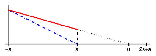
Figure 1. Exponents $0\leq\kappa\leq 1$ of $\|x_{\alpha}^{\delta}-x^{\dagger}\|_{\mathcal{X}_{r}}=O(\delta^{\kappa})$ as $\delta~{}\to~{}0$ under the assumption that $x^{\dagger}\in\mathcal{D}(F)\cap\mathcal{X}_{u}$. Estimate (1.5) of Theorems 1.1 and 1.2 (blue, dashed); estimate (2.1) obtained by a-priori and a-posteriori parameter choice in Theorems 2.1 and 2.2 (red).

Note that we obtain better convergence rates than predicted by Theorem 1.1, whenever $x^{\dagger}\in\mathcal{X}_{u}$ with $u>s$. Let us also mention that similar results were obtained by Tautenhahn [15] under stronger assumptions on the problem, i.e., under a Lipschitz stability condition for the inverse problem, further nonlinearity conditions on the operator $F$, and using an exact minimization of the Tikhonov functional in the definition of $x_{\alpha}^{\delta}$.

The remainder of the manuscript is organized as follows: In Sections 2 and 3, we state and prove our main results. The relation to previous results on regularization in Hilbert scales will be discussed in Section 4. Section 5 presents two model problems, for which our results apply, and in Section 6 we illustrate our theoretical results by numerical tests. The presentation closes with a short discussion of open topics.

2. Statement of the main results

We now state our main results, which can be seen as a generalization and improvement of the estimates of Theorem 1.1 for smooth solutions $x^{\dagger}\in\mathcal{X}_{u}$ with $u>s$.

Theorem 2.1 (A-priori parameter choice).

Let (A1)–(A2) hold and assume that $x^{\dagger}\in\mathcal{D}(F)\cap\mathcal{X}_{u}$ for some $-a\leq s\leq u\leq 2s+a$. Then for any $x_{\alpha}^{\delta}\in\mathcal{X}(\alpha;y^{\delta})$ with $\alpha=\delta^{2-2\gamma\frac{u-s}{u+a}}$ one has

(2.1) $$\|x_{\alpha}^{\delta}-x^{\dagger}\|_{\mathcal{X}_{r}}\leq C_{5}\delta^{\gamma\frac{u-r}{u+a}}\qquad\text{for all }-a\leq r\leq s$$

and $\|F(x_{\alpha}^{\delta})-y^{\delta}\|_{\mathcal{Y}}\leq C_{6}\delta$ with $C_{5},C_{6}$ depending only on the norm $\|x^{\dagger}\|_{\mathcal{X}_{u}}$

For the limiting case $u=s$, we recover the assertions of Theorem 1.1. Also note that Theorem 2.1 is yet not fully practical, since the a-priori parameter choice still requires knowledge of the smoothness index $u$ of the true solution which is not known in practice. An a-posteriori parameter choice strategy that does not require such knowledge is the discrepancy principle [10]. Here we consider the following strategy adopted to our setting: For $n\geq 0$ set $\alpha_{n}=2^{-n}$ and choose $x_{\alpha_{n}}^{\delta}\!\in X(\alpha_{n};y^{\delta})$. Based on this sequence $\{x_{\alpha_{n}}^{\delta}\!\}_{n\geq 0}$, we define

(2.2) $$n^{*}:=\inf\{n\geq 0:\|F(x_{\alpha_{n}}^{\delta}\!)-y^{\delta}\|_{\mathcal{Y}}\leq 4\delta\},$$

and we consider $\alpha=\alpha_{n^{*}}$ as the regularization parameter for determing a stable approximation for the solution of the inverse problem (1.1). This parameter choice strategy is computationally attractive since one can start generation of $x_{\alpha_{n}}^{\delta}\!$ with large $\alpha_{n}$, proceed to smaller $\alpha_{n}$, and stop as soon as the data residual reaches the desired tolerance. With this simple procedure, we already obtain the following result.

Theorem 2.2 (A-posteriori parameter choice).

Let (A1)–(A2) hold, define $n^{*}$, $\alpha_{n^{*}}$ as above, and assume that $x^{\dagger}\in\mathcal{D}(F)\cap\mathcal{X}_{u}$ for some $-a\leq s\leq u\leq 2s+a$. Then for any $x_{\alpha}^{\delta}\in\mathcal{X}(\alpha_{n^{*}};y^{\delta})$ the rates (2.1) hold with a constant $C_{5}$ depending only on $\|x^{\dagger}\|_{\mathcal{X}_{u}}$. Moreover, we have $\|F(x_{\alpha}^{\delta})-y^{\delta}\|_{\mathcal{Y}}\leq 4\delta$.

Note that no information about the actual smoothness of $x^{\dagger}$ is required in order to carry out the computations. Theorems 2.1 and 2.2 therefore yield a generalization and a true improvement of Theorem 1.1 for smooth solutions $x^{\dagger}\in\mathcal{X}_{u}$ with $u>s$.

3. Proof of the main results

This section is devoted to the proofs of Theorems 2.1 and 2.2. Throughout this section, we will always assume that assumptions (A1)–(A2) are valid and we assume that $-a\leq s\leq u\leq 2s+a$. Let us start with some preliminary observations and auxiliary a-priori estimates. From the definition of the set $\mathcal{X}(\alpha;y^{\delta})$ and the estimates in the proof of Theorem 1.1, we directly obtain the following results.

Lemma 3.1.

Let $x^{\dagger}\in\mathcal{D}(F)\cap\mathcal{X}_{s}$. Then $\mathcal{X}(\alpha;y^{\delta})$ is non-empty for any $\alpha\geq 0$. Moreover, we have $x^{\dagger}\in\mathcal{X}(\alpha;y^{\delta})$ if $\alpha$ is chosen sufficiently small.

From the estimates derived in the proof of Theorem 1.1, we also obtain the following a-priori estimates for the data residuals and the approximate minimizers.

Lemma 3.2.

Let $x^{\dagger}\in\mathcal{D}(F)\cap\mathcal{X}_{s}$ with $\|x^{\dagger}\|_{\mathcal{X}_{s}}=M$ and let $\tau>0$ be arbitrary. Then

• $\|F(x_{\alpha}^{\delta})-y^{\delta}\|_{\mathcal{Y}}^{2}\leq(2+\tau)\delta^{2}$ for all $\alpha\leq\tau\delta^{2}/M^{2}$;

• $\|x_{\alpha}^{\delta}\|_{\mathcal{X}_{s}}^{2}\leq(1+\frac{2}{\tau})M^{2}$ when $\alpha\geq\tau\delta^{2}/M^{2}$.

The parameter $\tau$ was introduced here only to have some flexibility that will be required in our proofs further below. In order to establish the improved convergence rates (2.1), we will need the following more accurate a-priori estimates.

Lemma 3.3.

Let $x^{\dagger}\in\mathcal{D}(F)\cap\mathcal{X}_{u}$ with $s<u\leq 2s+a$ and let $x_{\alpha}^{\delta}\in\mathcal{X}(\alpha;y^{\delta})$ for some parameter $\alpha\geq C\delta^{2}$ with $C>0$ only depending on $\|x^{\dagger}\|_{\mathcal{X}_{u}}$. Then

(3.1) $$\|F(x_{\alpha}^{\delta})-F(x^{\dagger})\|_{\mathcal{Y}}^{2}+\alpha\|x_{\alpha}^{\delta}-x^{\dagger}\|_{\mathcal{X}_{s}}^{2}\leq 12\delta^{2}+C_{7}\alpha^{\frac{u+a}{u+a-\gamma(u-s)}}$$

with constant $C_{7}$ only depending on the size of $\|x^{\dagger}\|_{\mathcal{X}_{u}}$.

Proof.

From the lower bound bound on $\alpha$ stated in the assumptions, the definition of $x_{\alpha}^{\delta}$, and the second estimate of Lemma 3.2, one can see that $x_{\alpha}^{\delta}\in\mathcal{D}(F)\cap\mathcal{X}_{s}$ with $\|x_{\alpha}^{\delta}\|_{\mathcal{X}_{s}}\leq M_{1}$ for some constant $M_{1}$ only depending on the norm $\|x^{\dagger}\|_{\mathcal{X}_{u}}$. With similar arguments as in the proof of [6, Thm. 10.4], we then get

(3.2) $$\frac{1}{2}\|F(x_{\alpha}^{\delta}) -F(x^{\dagger})\|_{\mathcal{Y}}^{2}+\alpha\|x_{\alpha}^{\delta}-x^{\dagger}\|^{2}_{\mathcal{X}_{s}}$$

$$\leq\|F(x_{\alpha}^{\delta})-y^{\delta}\|_{\mathcal{Y}}^{2}+\delta^{2}+\alpha\|x_{\alpha}^{\delta}-x^{\dagger}\|^{2}_{\mathcal{X}_{s}}$$

$$\leq\|F(x^{\dagger})-y^{\delta}\|^{2}_{\mathcal{Y}}+2\delta^{2}+2\alpha(x^{\dagger},x^{\dagger}-x_{\alpha}^{\delta})_{\mathcal{X}_{s}}$$

$$\leq 3\delta^{2}+2\alpha\|x^{\dagger}\|_{\mathcal{X}_{u}}\|x_{\alpha}^{\delta}-x^{\dagger}\|_{\mathcal{X}_{2s-u}}.$$

Here we used (A1) in the first inequality, the definition of $x_{\alpha}^{\delta}$ and some basic computations for the second estimate, and assumption (A1) as well as a Cauchy-Schwarz-type inequality in the third step. Application of the interpolation inequality (1.4) with $p=-a$, $q=2s-u$, and $r=s$, further noting that $\|x_{\alpha}^{\delta}\|_{\mathcal{X}_{s}}\leq M_{1}$ and $\|x^{\dagger}\|_{\mathcal{X}_{s}}\leq\|x^{\dagger}\|_{\mathcal{X}_{u}}\leq M_{1}$ w.l.o.g., and using the stability estimate (A2) yields

$$\|x_{\alpha}^{\delta}-x^{\dagger}\|_{\mathcal{X}_{2s-u}} \leq\|x_{\alpha}^{\delta}-x^{\dagger}\|_{\mathcal{X}_{-a}}^{\frac{u-s}{s+a}}\|x_{\alpha}^{\delta}-x^{\dagger}\|_{\mathcal{X}_{s}}^{\frac{2s+a-u}{s+a}}$$

$$\leq R(M_{1})^{\frac{u-s}{s+a}}\|F(x_{\alpha}^{\delta})-F(x^{\dagger})\|_{\mathcal{Y}}^{\gamma\frac{u-s}{s+a}}\|x_{\alpha}^{\delta}-x^{\dagger}\|_{\mathcal{X}_{s}}^{\frac{2s+a-u}{s+a}}.$$

This allows us to bound the last term in the estimate (3.2) by

(3.3) $$2\alpha\|x^{\dagger}\|_{\mathcal{X}_{u}}\|x_{\alpha}^{\delta}-x^{\dagger}\|_{\mathcal{X}_{2s-u}}$$

$$\leq\big{(}C^{\prime}\alpha^{\frac{u+a}{2s+2a}}\|x^{\dagger}\|_{\mathcal{X}_{u}}\big{)}\cdot\big{(}\alpha^{\frac{2s+a-u}{2s+2a}}\|x_{\alpha}^{\delta}-x^{\dagger}\|_{\mathcal{X}_{s}}^{\frac{2s+a-u}{s+a}}\big{)}\cdot\big{(}\|F(x_{\alpha}^{\delta})-F(x^{\dagger})\|^{\gamma\frac{u-s}{s+a}}\big{)},$$

with constant $C^{\prime}$ only depending on $\|x^{\dagger}\|_{\mathcal{X}_{u}}$. By Young’s inequality, one can see that

$$a\cdot b\cdot c\leq\frac{a^{p}}{p}+\frac{b^{q}}{q}+\frac{c^{r}}{r}$$

for all $a,b,c\geq 0$ and $1\leq p,q,r\leq\infty$ with $\frac{1}{p}+\frac{1}{q}+\frac{1}{r}=1$. Applying this inequality with indices $p=\frac{2s+2a}{u+a-\gamma(u-s)}$, $q=\frac{2s+2a}{2s+a-u}$, and $r=\frac{2}{\gamma}\frac{s+a}{u-s}$ in the estimate (3.3) leads to

$$2\alpha\|x^{\dagger}\|_{\mathcal{X}_{u}} \|x_{\alpha}^{\delta}-x^{\dagger}\|_{\mathcal{X}_{2s-u}}$$

$$\leq C^{\prime\prime}\alpha^{\frac{u+a}{u+a-\gamma(u-s)}}+\tfrac{3\alpha}{4}\|x_{\alpha}^{\delta}-x^{\dagger}\|_{\mathcal{X}_{s}}^{2}+\tfrac{1}{4}\|F(x_{\alpha}^{\delta})-F(x^{\dagger})\|^{2}_{\mathcal{Y}},$$

with $C^{\prime\prime}$ depending on $\|x^{\dagger}\|_{\mathcal{X}_{u}}$ and on the indices $a,s,u$, and $\gamma$. The last two terms can then be absorbed in the left hand side of (3.2). This yields the estimate of the lemma with constant $C_{7}=4C^{\prime\prime}$ and concludes the proof. ∎

Proof of Theorem 2.1.

A combination of Lemma 3.3 with the a-priori parameter choice $\alpha=\delta^{2-2\gamma\frac{u-s}{u+a}}$ yields $\|F(x_{\alpha}^{\delta})-F(x^{\dagger})\|_{\mathcal{Y}}\leq C\delta$ and $\|x_{\alpha}^{\delta}-x^{\dagger}\|_{\mathcal{X}_{s}}\leq C^{\prime}\delta^{\gamma\frac{u-s}{u+a}}$. Using assumption (A2), we also obtain $\|x_{\alpha}^{\delta}-x^{\dagger}\|_{\mathcal{X}_{-a}}\leq C^{\prime\prime}\delta^{\gamma}$. By the interpolation inequality (1.4), we then obtain $\|x_{\alpha}^{\delta}-x^{\dagger}\|_{\mathcal{X}_{r}}\leq C_{5}\delta^{\gamma\frac{u-r}{u+a}}$, and using (A1) and the triangle inequality yields $\|F(x_{\alpha}^{\delta})-y^{\delta}\|_{\mathcal{Y}}\leq C_{6}\delta$. ∎

Let us now turn to the proof of Theorem 2.2. As a consequence of Lemma 3.1, we can find for any $n\geq 0$ an approximate solution $x_{\alpha_{n}}^{\delta}\!\in\mathcal{X}(\alpha_{n};y^{\delta})$ where $\alpha_{n}=2^{-n}$. Using Lemma 3.2, one can see that $n^{*}$ is well-defined by the stopping rule (2.2) and finite, once a sequence of approximate solutions $x_{\alpha_{n}}^{\delta}\!\in\mathcal{X}(\alpha_{n};y^{\delta})$ has been chosen. In addition, we have the following preliminary lower bound.

Lemma 3.4.

Let $n^{*}$ be chosen by (2.2). Then $\alpha_{n^{*}}\geq 7\delta^{2}/M^{2}$ and $\|x_{\alpha_{n^{*}}}^{\delta}\!\|_{\mathcal{X}_{s}}^{2}\leq 2M^{2}$ for all $x_{\alpha}^{\delta}\in\mathcal{X}(\alpha_{n^{*}};y^{\delta})$. As before, $M=\|x^{\dagger}\|_{\mathcal{X}_{s}}$ is the norm of the true solution.

Proof.

From Lemma 3.2, we deduce that $\|F(x_{\alpha_{n}}^{\delta}\!)-y^{\delta}\|_{\mathcal{Y}}>4\delta$ can only happen, when $\alpha_{n}>14\delta^{2}/M^{2}$. This condition must particularly hold for $n=n^{*}-1$, which already implies the lower bound for $\alpha_{n^{*}}$. The bound for $\|x_{\alpha_{n^{*}}}^{\delta}\!\|_{\mathcal{X}_{s}}$ then follows from the second assertion of Lemma 3.2 with $\tau=7$. ∎

As a direct consequence of the estimates of Lemma 3.3, we obtain the following sharper bound for the regularization parameter from below.

Lemma 3.5.

The regularization parameter determined by (2.2) satisfies

$$\alpha_{n^{*}}\geq C_{8}\delta^{2-2\gamma\frac{u-s}{a+u}}$$

with constant $C_{8}$ only depending on the norm $\|x^{\dagger}\|_{\mathcal{X}_{u}}$ of the exact solution.

As a final ingredient for the proof of Theorem 2.2, we require the following estimate for a term that already appeared in the proof of Lemma 3.3.

Lemma 3.6.

Assume that $\|F(x_{\alpha}^{\delta})-y^{\delta}\|_{\mathcal{Y}}\leq 4\delta$ and $\alpha\geq C_{8}\delta^{2-2\gamma\frac{u-s}{a+u}}$. Then

$$2\|x^{\dagger}\|_{\mathcal{X}_{u}}\|x_{\alpha}^{\delta}-x^{\dagger}\|_{\mathcal{X}_{2s-u}}\leq C_{9}\delta^{2\gamma\frac{u-s}{a+u}}+\tfrac{a+2s-u}{2a+2s}\|x_{\alpha}^{\delta}-x^{\dagger}\|^{2}_{\mathcal{X}_{s}}$$

with constant $C_{9}$ depending only on the norm $M=\|x^{\dagger}\|_{\mathcal{X}_{u}}$ of the exact solution.

Proof.

With similar arguments as in the proof of Lemma 3.3, we obtain by the interpolation inequality (1.4) with $p=-a$, $q=2s-u$, $r=s$, the bound

$$2\|x^{\dagger}\|_{\mathcal{X}_{u}}\|x_{\alpha}^{\delta}-x^{\dagger}\|_{\mathcal{X}_{2s-u}}$$

$$\qquad\leq 2M\|x_{\alpha}^{\delta}-x^{\dagger}\|^{\frac{u-s}{a+s}}_{\mathcal{X}_{-a}}\|x_{\alpha}^{\delta}-x^{\dagger}\|_{\mathcal{X}_{s}}^{2}\big{)}^{\frac{a+2s-u}{2a+2s}}.$$

An application of Young’s inequality $a\cdot b\leq\frac{a^{p}}{p}+\frac{b^{q}}{q}$ with $p=\frac{2a+2s}{a+u}$ and $q=\frac{2a+2s}{a+2s-u}$ further yields

$$(*)\leq C^{\prime}(M)\|x_{\alpha}^{\delta}-x^{\dagger}\|_{\mathcal{X}_{-a}}^{2\frac{u-s}{a+u}}+\frac{1}{2}\|x_{\alpha}^{\delta}-x^{\dagger}\|^{2}_{\mathcal{X}_{s}}$$

with constant $C^{\prime}(M)$ depending only on $M$. From the stability condition (A2) and using $\|x^{\dagger}\|_{\mathcal{X}_{s}}\leq\|x^{\dagger}\|_{\mathcal{X}_{u}}=M$, we deduce that

$$\|x_{\alpha}^{\delta}-x^{\dagger}\|_{\mathcal{X}_{-a}}^{2\frac{u-s}{a+u}}\leq R(M)^{2\frac{u-s}{a+u}}\|F(x_{\alpha}^{\delta})-F(x^{\dagger})\|^{2\gamma\frac{u-s}{a+u}}\leq C^{\prime\prime}(M)\delta^{2\gamma\frac{u-s}{a+u}}.$$

Here we employed that $\|F(x_{\alpha}^{\delta})-F(x^{\dagger})\|_{\mathcal{Y}}\leq 5\delta$ which follows from condition (A1) and the assumption of the lemma via the triangle inequality. The assertion of the lemma now follows directly from the previous estimates. ∎

Proof of Theorem 2.2.

From the estimate (3.2) which was derived in the proof of Lemma 3.3, we can deduce that

$$\alpha\|x_{\alpha}^{\delta}-x^{\dagger}\|^{2}_{\mathcal{X}_{s}}\leq 2\delta^{2}+2\alpha\|x^{\dagger}\|_{\mathcal{X}_{u}}\|x_{\alpha}^{\delta}-x^{\dagger}\|_{\mathcal{X}_{2s-u}}.$$

Dividing by $\alpha$ and using Lemma 3.6 to estimate the last term yields

$$\tfrac{a+u}{2a+2s}\|x_{\alpha}^{\delta}-x^{\dagger}\|^{2}_{\mathcal{X}_{s}}\leq 2\delta^{2}/\alpha+C_{9}\delta^{2\gamma\frac{u-s}{a+u}}.$$

From the condition $-a\leq s\leq u\leq 2a+2s$ one can see that $\frac{u+a}{2a+2s}\geq\frac{1}{2}$. Using this fact, the bound $\alpha=\alpha_{n^{*}}\geq C_{8}\delta^{2-2\gamma\frac{u-s}{a+u}}$ provided by Lemma 3.5, and taking the square root then yields the estimate $\|x_{\alpha}^{\delta}-x^{\dagger}\|_{\mathcal{X}_{s}}\leq C_{5}\delta^{\gamma\frac{u-s}{u+a}}$. The estimate $\|x_{\alpha}^{\delta}-x^{\dagger}\|_{\mathcal{X}_{-a}}\leq C_{5}\delta^{\gamma}$ follows from assumptions (A2), (A2), and the discrepancy rule, which yield $\|F(x_{\alpha}^{\delta})-F(x^{\dagger})\|_{\mathcal{Y}}\leq\|F(x_{\alpha}^{\delta})-y^{\delta}\|_{\mathcal{Y}}+\delta\leq 5\delta$. The estimate for $\|x_{\alpha}^{\delta}-x^{\dagger}\|_{\mathcal{X}_{r}}$ is the again obtained by interpolation. ∎

4. Remarks on regularization in Hilbert scales

Now we are going to recall some previous results about regularization in Hilbert scales and illustrate their relation to those established in this paper. Let us start with linear inverse problems $Tx=y$ with bounded linear forward operators $T$ mapping from $\mathcal{X}$ to $\mathcal{Y}$, and consider data $y^{\delta}\in\mathcal{Y}$ satisfying assumption (A1). For the stable solution, we again consider Tikhonov regularization in Hilbert scales for $s\geq 0$ with regularized approximations $x_{\alpha}^{\delta}$ defined by

$$x_{\alpha}^{\delta}=\text{argmin}\,\{\|Tx-y^{\delta}\|_{\mathcal{Y}}^{2}+\alpha\|x\|^{2}_{\mathcal{X}_{s}}\}.$$

The basic assumption for the convergence analysis in the linear case is that the operator $T$ admits a two-sided estimate of the form

(4.1) $$\underline{c}\|x\|_{\mathcal{X}_{-a}}\leq\|Tx\|_{\mathcal{Y}}\leq\overline{c}\|x\|_{\mathcal{X}_{-a}},$$

for some parameter $a\geq 0$ characterizing the degree of ill-posedness of the inverse problem. If the true solution satisfies $x^{\dagger}\in\mathcal{X}_{u}$ for some $u$ satisfying $-a\leq u\leq 2s+a$ and if the regularization parameter is chosen as

(4.2) $$\alpha=\delta^{\frac{2(a+s)}{a+u}}\,,$$

then one obtains the optimal convergence rates

(4.3) $$\|x^{\dagger}-x_{\alpha}^{\delta}\|_{\mathcal{X}_{r}}\leq C\delta^{\frac{u-r}{a+u}}\qquad\mbox{for all}\qquad-a\leq r\leq u\leq a+2s;$$

see [11] or [6, Rem. 8.24] for details. For $s\leq u$ these estimates and also the parameter choice coincide with the ones of Theorem 2.1 in the case $\gamma=1$, where (A2) describes the Lipschitz stability of the inverse problem. Vice versa, assumption (4.1) also implies the validity of the condition (A2) with exponent $\gamma=1$.

Remark 4.1.

The convergence rate result (4.3) remains true also in the oversmoothing case $s>u\geq-a$, where $\|x^{\dagger}\|_{\mathcal{X}_{s}}=\infty$; see [7] for an extension to nonlinear problems. Also note that in the oversmoothing case with $\alpha$ chosen by (4.2), we have

$$\lim\limits_{\delta\to 0}\frac{\delta^{2}}{\alpha}=\delta^{\frac{2(u-s)}{a+u}}=+\infty,$$

whereas for $u=s,\;\|x^{\dagger}\|_{\mathcal{X}_{s}}<\infty$ and $0<\gamma\leq 1$, which is considered in Theorems 1.1 and 1.2 as well as e.g. [2], one obtains

$$\underline{c}\leq\frac{\delta^{2}}{\alpha}\leq\overline{c}\quad\mbox{for constants}\quad 0<\underline{c}\leq\overline{c}<\infty.$$

The results of Theorem 2.1 cover the third case $u>s,\;\|x^{\dagger}\|_{\mathcal{X}_{s}}<\infty$, and $0<\gamma\leq 1$, and yield the asymptotic behavior

$$\lim\limits_{\delta\to 0}\frac{\delta^{2}}{\alpha}=\delta^{\frac{2\gamma(u-s)}{a+u}}=0.$$

This is the condition for an a-priori parameter choice that is is required to ensure convergence of Tikhonov regularization in Hilbert spaces; see [6].

Using the interpolation inequality (1.4) and the first estimate in (4.1), we can also obtain a conditional Hölder stability estimate of the form

$$\|x_{1}-x_{2}\|_{\mathcal{X}_{-q}}\leq\|x_{1}-x_{2}\|_{\mathcal{X}_{-a}}^{\frac{s+q}{s+a}}\|x_{1}-x_{2}\|_{\mathcal{X}_{s}}^{\frac{a-q}{s+a}}\leq R(\rho)\|Tx_{1}-Tx_{2}\|_{\mathcal{Y}}^{\gamma},$$

which is valid for all $-a\leq-q\leq s$, for all $x_{1},x_{2}\in\mathcal{X}_{s}$ with $\|x_{i}\|_{\mathcal{X}_{s}}\leq\rho$ and for constants $R(\rho)=2\rho^{1-\gamma}\underline{c}^{-\gamma}$ and $\gamma=\frac{s+q}{s+a}$. Note that this stability estimate is strictly weaker than (4.1) whenever $a>q$. For the case $u=s$, Theorem 2.1 however still yields the same parameter choice and the order optimal convergence rates as described above.

If $u>s$, then the convergence rates predicted Theorem 2.1 are somewhat smaller; see also our discussion at the end of Section 6.1. In view of Figure 1, the rates are however still order optimal under the given assumptions. Theorems 2.2 and 2.1 can therefore be understood as true generalizations, with respect to varying $0<\gamma\leq 1$, of the results about Tikhonov regularization in Hilbert scales from [11] and [6].

Let us now turn to operator equations (1.1) with nonlinear operator $F$. The essential condition for the analysis of Tikhonov regularization in Hilbert scales used in [13] here reads as

$$\underline{c}\|h\|_{\mathcal{X}_{-a}}\leq\|F^{\prime}(x)h\|_{\mathcal{Y}}\leq\overline{c}\|h\|_{\mathcal{X}_{-a}}\quad\text{for all }\;\;x\in\mathcal{D}(F)\cap\mathcal{X}_{s}.$$

By Taylor expansion and the triangle inequality, one can see that

(4.4) $$\underline{c}\|x_{1} -x_{2}\|_{\mathcal{X}_{-a}}\leq\|F(x_{1})-F(x_{2})\|_{\mathcal{Y}}$$

$$+\|\int_{0}^{1}[F^{\prime}(x_{1})-F^{\prime}(x_{1}+t(x_{1}-x_{2}))](x_{1}-x_{2})dt\|_{\mathcal{Y}}.$$

To obtain quantitative estimates for regularization in Hilbert scales, one should additionally assume that the derivative is at least Hölder continuous, i.e.,

$$\|[F^{\prime}(x)-F^{\prime}(\tilde{x})]\,h\|_{\mathcal{Y}}\leq C\|x-\tilde{x}\|_{\mathcal{X}_{r}}^{\beta}\|h\|_{\mathcal{X}_{-a}},$$

for all $x,\tilde{x}\in\mathcal{D}(F)\cap\mathcal{X}_{s}$ and $h\in\mathcal{X}_{-a}$ with some $-a\leq r\leq s$ and some $\beta>0$. We refer to [4, 14] for details. The last term in (4.4) can then be absorbed into the left hand side of the estimate. This yields the stability assumption (A2) with $\gamma=1$ for all $x_{1},x_{2}\in\mathcal{X}_{s}\cap\mathcal{D}(F)$ with $\|x_{1}\|_{\mathcal{X}_{s}},\|x_{2}\|_{\mathcal{X}_{s}}\leq\rho$ and $\|x_{1}-x_{2}\|_{-a}$ sufficiently small. The resulting estimates of Theorem 2.2 and 2.1 then again coincide with the ones obtained in [13] under the nonlinearity conditions stated above.

Let us finally note that the stability condition (A2) does in general not even imply continuity or differentiability of the forward operator $F$. Both Theorems 2.2 and 2.1 therefore cover rather general problems and the results of this paper can be seen as a true generalization of previous results about regularization in Hilbert scales.

5. Model problems

For illustration of the applicability of our results and as model scenarios for our numerical tests, we consider the following two simple test problems.

5.1. Data smoothing

Let $H^{r}_{per}(0,2\pi)=\{f(x)=\sum_{k\in\mathbb{Z}}f_{k}e^{ikx}:\|f\|_{r}<\infty\}$ denote the space of $2\pi$-periodic functions with bounded norm $\|f\|_{r}^{2}=\sum_{k}(1+k^{2})^{r}|f_{k}|^{2}$. We consider the reconstruction of a signal $f$ from noisy measurements $f^{\delta}$ with noise bounded by $\|f^{\delta}-f\|_{-1}\leq\delta$; this allows for irregular and possibly large noise [5]. The corresponding inverse problem then reads as follows: Find $f\in H^{0}_{per}(0,1)$ such that the corresponding operator $T$ in the linear operator equation is defined by

$$T:H^{0}_{per}(0,2\pi)\to H^{-1}_{per}(0,2\pi),\quad f\mapsto f.$$

Note that the reconstruction will be based on noisy observation $f^{\delta}$ for the true solution $f^{\dagger}$. Using interpolation in the frequency domain, one can see that

$$\|f\|_{0}\leq\|f\|_{r}^{\frac{1}{r+1}}\|f\|_{-1}^{\frac{r}{r+1}},$$

for all $r\geq 0$ and all $f\in H^{r}_{per}(0,2\pi)$. By the linearity of the problem and this interpolation estimate, we obtain for $r=1$ and for all $f_{1},f_{2}\in H_{per}^{2}(0,2\pi)$ that

$$\|f_{1}-f_{2}\|_{0}\leq(\|f_{1}\|_{1}+\|f_{2}\|_{1})^{1/2}\|Tf_{1}-Tf_{2}\|_{-1}^{1/2}.$$

This exactly amounts to the stability condition (A2) with spaces $\mathcal{X}_{s}=H^{s}_{per}(0,2\pi)$, $\mathcal{Y}=H^{-1}_{per}(0,2\pi)$, and parameters $a=0$, $s=1$, $\gamma=1/2$ and $R(\rho)=(2\rho)^{1/2}$.

Remark 5.1.

For the data smoothing problem, we also have the two-sided estimate

$$\|f\|_{-1}\leq\|Tf\|_{\mathcal{Y}}\leq\|f\|_{-1},$$

which amounts to (4.1) with $a=1$ and which also implies (A2) with this value $a$ and $\gamma=1$. For evaluation of our results, we will make use of this Lipschitz stability estimate as well as of the Hölder stability estimate above in our numerical tests.

5.2. Parameter identification

As a second model problem, we consider a coefficient inverse problem for a parabolic equation similar to an example in [9]. We use different boundary conditions here, which allows us to provide simpler proofs.

Let $\Omega\subset\mathbb{R}^{d}$ denote a bounded sufficiently regular domain. We consider a reaction-diffusion problem of the form

$$\partial_{t}u-\Delta u+cu =0\qquad\text{in }\Omega,$$

$$\partial_{n}u =0\qquad\text{on }\partial\Omega,$$

for all $$0<t\leq T$$ and with given initial values given by

$$u(\cdot,0) =u_{0}\quad\;\;\text{in }\Omega.$$

We assume that $u_{0}$ is sufficiently smooth and that the parameter $c=c(t)$ is independent of space. The goal here is to identify this parameter $c$ from measurements of $U=\int_{\Omega}u(x,\cdot)dx$. This amounts to an inverse problem $F(c)=U^{\delta}$ with operator

$$F:\mathcal{D}(F)\subset L^{2}(0,T)\to L^{2}(0,T),\qquad c\mapsto\int_{\Omega}u(x,\cdot)dx$$

It is not difficult to see that $F$ is well-defined on $\mathcal{D}(F)=\{c\in L^{2}(0,T):c\geq 0\}$. Using $U=\int_{\Omega}u(x,\cdot)dx$ and integrating the differential equation over $\Omega$, we obtain

$$U^{\prime}+cU =0,\ t>0\qquad\text{with}\qquad U(0)=\int_{\Omega}u_{0}(x)dx.$$

The solution is then given by $U(t)=U(0)e^{-\int_{0}^{t}c(s)ds}$, which shows that $|U(t)|$ is monotonically decreasing since we assumed $c\geq 0$. As a consequence, we obtain

$$e^{-\sqrt{T}\|c\|_{L^{2}(0,T)}}|U(0)|\leq|U(t)|\leq|U(0)|.$$

In particular, $U(t)\neq 0$ whenever $U(0)\neq 0$, which we assume in the following. Using the differential equation repeatedly, one can obtain estimates for the derivatives

$$\|U^{\prime}\|_{L^{2}(0,T)} \leq|U(0)|\|c\|_{L^{2}(0,T)},$$

$$\|U^{\prime\prime}\|_{L^{2}(0,T)} \leq|U(0)|\big{(}C_{T}\|c\|_{H^{1}(0,T)}\|c\|_{L^{2}(0,T)}+\|c\|_{H^{1}(0,T)}\big{)}.$$

In a similar way one can estimate $\|U\|_{H^{s+1}(0,T)}$ by powers $\|c\|_{H^{s}(0,T)}$ for $s\geq 0$. Now let $U_{1},U_{2}$ denote two measurements resulting from coefficients $c_{1},c_{2}$ but with the same initial data $U_{1}(0)=U_{2}(0)=U(0)$. Then the difference $W=U_{1}-U_{2}$ satisfies

$$W^{\prime}+c_{1}W =(c_{2}-c_{1})U_{2},\ t>0\qquad\text{and}\qquad W(0)=0.$$

From this equation and the uniform bounds for the functions $F(c_{i})=U_{i}$ one can see that $F$ is continuous and weakly closed. Using $U(0)\neq 0$ and the monotonicity of $|U(t)|$, one can further deduce that

$$\|c_{1}-c_{2}\|_{L^{2}(0,T)} \leq\frac{1}{|U_{2}(T)|}\big{(}\|W^{\prime}\|_{L^{2}(0,T)}+\|c_{1}\|_{L^{2}(0,T)}\|W\|_{L^{\infty}(0,T)}\big{)}$$

$$\leq e^{\sqrt{T}\|c_{2}\|_{L^{2}(0,T)}}(1+C_{T}\|c_{1}\|_{L^{2}(0,T)})\|F(c_{1})-F(c_{2})\|_{H^{1}(0,T)}.$$

For the last step, we used the embedding of $H^{1}(0,T)$ into $L^{\infty}(0,T)$ here. By interpolation of Sobolev spaces, we further obtain

$$\|F(c_{1})-F(c_{2})\|_{H^{1}(0,T)}\leq C_{s}\|F(c_{1})-F(c_{2})\|_{L^{2}(0,T)}^{\frac{s}{s+1}}\|F(c_{1})-F(c_{2})\|_{H^{s+1}(0,T)}^{\frac{1}{s+1}},$$

which holds for any parameter $s\geq 0$. Using the bounds for $U_{i}=F(c_{i})$ to estimate the term $\|F(c_{1})-F(c_{2})\|_{H^{s+1}(0,T)}$, we then get

$$\|c_{1}-c_{2}\|_{L^{2}(0,T)} \leq R(\rho)\|F(c_{1})-F(c_{2})\|_{L^{2}(0,T)}^{\frac{s}{s+1}}$$

for all $\|c_{1}\|_{H^{s}(0,T)},\|c_{2}\|_{H^{s}(0,T)}\leq\rho$ and with appropriate function $R(\rho)$. This is exactly the conditional stability estimate (A2) required for our analysis.

Remark 5.2.

One can see that $F$ is also differentiable with $F^{\prime}(c)h=W$ defined by

$$W^{\prime}+cW=-hU,\ t>0,\qquad W(0)=0,$$

and with function $U=F(c)$ defined as before. By the variation-of-constants formula, one obtains $W(t)=\int_{0}^{t}e^{-\int_{s}^{t}c(r)dr}h(s)U(s)ds$, which shows that

$$\|W\|_{L^{\infty}(0,T)}\leq\|hU\|_{L^{1}(0,T)}\leq\|h\|_{L^{1}(0,T)}|U(0)|.$$

By embedding of Sobolev spaces, one can then obtain an upper estimate

$$\|F^{\prime}(c)h\|_{L^{2}(0,T)}=\|W\|_{L^{2}(0,T)}\leq\overline{c}\|h\|_{L^{2}(0,T)}.$$

From the explicit representation of the function $W=F^{\prime}(c)h$ one can however see that an estimate $\underline{c}\|h\|_{L^{2}(0,T)}\leq\|F^{\prime}(c)h\|_{L^{2}(0,T)}$ from below is certainly not valid. Previous results on regularization in Hilbert scales are therefore not applicable directly.

6. Numerical tests

We now illustrate the results Theorems 2.2 and 2.1 by some numerical tests. As model problems, we consider the ones introduced in the previous section.

6.1. Data smoothing

As a first test case, we consider the problem described in Section 5.1 and we utilize the Lipschitz stability condition

(6.1) $$\|f_{1}-f_{2}\|_{-1}\leq\|Tf_{1}-Tf_{2}\|_{-1}.$$

This corresponds to (A2) with $a=1$ and $\gamma=1$, and we may set $s\geq 0$ arbitrary. For our numerical tests, the functions $f$ are represented by piecewise linear splines over a uniform grid of $[0,2\pi]$. As reference solutions, we consider the functions

$$f^{\dagger}(t)=\begin{cases}0,&t<\pi,\\ 1,&t>\pi,\end{cases}\qquad f^{\dagger}(t)=\sqrt{t(2\pi-t)},\quad\text{and}\quad f^{\dagger}(t)=\begin{cases}t,&t<\pi,\\ 2\pi-t,&t>\pi,\end{cases}$$

which have different regularity. In the first case, $f^{\dagger}\in H^{u}_{per}(0,2\pi)$ for any $u<1/2$, in the second case, $f^{\dagger}\in H^{u}_{per}(0,2\pi)$ for all $u<1$, and in the third case, $f^{\dagger}\in H^{u}_{per}(0,2\pi)$ for all $u<3/2$. In Table 1 we list the parameter choices and convergence rates for these three cases predicted by our theory.

	$s=0$			$s=1$
$u$	$\alpha$	$\|f_{\alpha}^{\delta}-f^{\dagger}\|_{\mathcal{X}_{0}}$	$\|f_{\alpha}^{\delta}-f^{\dagger}\|_{\mathcal{X}_{1}}$	$\alpha$	$\|f_{\alpha}^{\delta}-f^{\dagger}\|_{\mathcal{X}_{0}}$	$\|f_{\alpha}^{\delta}-f^{\dagger}\|_{\mathcal{X}_{1}}$
$\frac{1}{2}$	$\delta^{4/3}$	$\delta^{1/3}$	—	$\delta^{8/3}$	$\color[rgb]{0,0,1}\delta^{1/3}$	—
$1$	$\delta$	$\delta^{1/2}$	$\color[rgb]{0,0,1}\delta^{0}$	$\delta^{2}$	$\delta^{1/2}$	$\delta^{0}$
$\frac{3}{2}$	$\delta^{4/5}$	$\color[rgb]{0,0,1}\delta^{3/5}$	$\color[rgb]{0,0,1}\delta^{1/5}$	$\delta^{8/5}$	$\delta^{3/5}$	$\delta^{1/5}$

Table 1. Parameter choice and convergence estimates of Theorem 2.1 for the data smoothing problem with assumption (A2) with $a=1,\gamma=1$. The results in blue are not covered by our theory since one of the conditions $s\leq u\leq 2s+a$ or $-a\leq r\leq s$ is violated.

Note that due to the restrictions $-a\leq r\leq s$ and $s\leq u\leq 2s+a$, not all results listed in the table are fully covered by our theory. In Tables 2, we list the results obtained in our numerical tests for the a-priori parameter choice.

	$s=0$			$s=1$
$u$	$\alpha$	$\|f_{\alpha}^{\delta}-f^{\dagger}\|_{\mathcal{X}_{0}}$	$\|f_{\alpha}^{\delta}-f^{\dagger}\|_{\mathcal{X}_{1}}$	$\alpha$	$\|f_{\alpha}^{\delta}-f^{\dagger}\|_{\mathcal{X}_{0}}$	$\|f_{\alpha}^{\delta}-f^{\dagger}\|_{\mathcal{X}_{1}}$
$\frac{1}{2}$	$\delta^{1.33}$	$\delta^{0.41}$	—	$\delta^{2.67}$	$\color[rgb]{0,0,1}\delta^{0.37}$	—
$1$	$\delta^{1.00}$	$\delta^{0.53}$	$\color[rgb]{0,0,1}\delta^{0.04}$	$\delta^{2.00}$	$\delta^{0.49}$	$\delta^{0.04}$
$\frac{3}{2}$	$\delta^{0.80}$	$\color[rgb]{0,0,1}\delta^{0.67}$	$\color[rgb]{0,0,1}\delta^{0.23}$	$\delta^{1.60}$	$\delta^{0.64}$	$\delta^{0.21}$

Table 2. Rates for a-priori parameter choice $\alpha=\delta^{2-2\gamma\frac{u-s}{u+a}}$ and reconstruction errors obtained in numerical tests for data smoothing problem with $a=1$ and $\gamma=1$. Results in red and blue are not covered by theory.

The observed convergence rates agree very well with the theoretical predictions. Although the condition $u\leq 2s+a$ is violated for the results of the last line for $s=0$, we still observe the optimal convergence rates also in that case. The results that are skipped correspond to negative rates or very large errors. In Table 3, we list the corresponding results obtained with the a-posteriori parameter choice.

	$s=0$			$s=1$
$u$	$\alpha$	$\|f_{\alpha}^{\delta}-f^{\dagger}\|_{\mathcal{X}_{0}}$	$\|f_{\alpha}^{\delta}-f^{\dagger}\|_{\mathcal{X}_{1}}$	$\alpha$	$\|f_{\alpha}^{\delta}-f^{\dagger}\|_{\mathcal{X}_{0}}$	$\|f_{\alpha}^{\delta}-f^{\dagger}\|_{\mathcal{X}_{1}}$
$\frac{1}{2}$	$\delta^{1.26}$	$\delta^{0.36}$	—	$\delta^{2.59}$	$\color[rgb]{0,0,1}\delta^{0.36}$	—
$1$	$\delta^{1.02}$	$\delta^{0.48}$	$\color[rgb]{0,0,1}\delta^{0.02}$	$\delta^{1.95}$	$\delta^{0.48}$	$\delta^{0.04}$
$\frac{3}{2}$	$\delta^{1.00}$	$\color[rgb]{0,0,1}\delta^{0.56}$	$\color[rgb]{0,0,1}\delta^{0.01}$	$\delta^{1.48}$	$\delta^{0.58}$	$\delta^{0.19}$

Table 3. Parameter choice and reconstruction errors for a-posteriori parameter choice for data smoothing problem using (A2) with $a=1,\gamma=1$. The results in red and blue are not covered by our theory since one of the conditions $s\leq u\leq 2s+a$ or $-a\leq r\leq s$ is violated.

Also here we observe the optimal convergence rates in good agreement with the theoretical predictions of Theorem 2.2. For the case $s=0$ and $u=3/2$, the condition $u\leq 2s+a$ is violated and we here observe a saturation phenomenon, i.e., for the choice $s=0$ smoothness higher than $u=1$ does not lead to a further improvement. This was not the case for the a-priori stopping rule. However, one can take advantage of higher smoothness here by regularizing in a stronger norm, e.g., with $s=1$, which restores the full convergence rate.

Before we proceed to the second test problem, let us make another observation. As outlined in the previous section, we can also use the Hölder stability estimate

(6.2) $$\|f_{1}-f_{2}\|_{0}\leq R(\rho)\|Tf_{1}-Tf_{2}\|_{-1}^{1/2}$$

for all $f_{1},f_{2}\in H^{1}_{per}(0,2\pi)$ with $\|f_{i}\|_{1}\leq\rho$ instead of the Lipschitz estimate (6.1). This amounts to the stability condition (A2) with $a=0$, $\gamma=1/2$, and $s=1$. The theoretical rates predicted by Theorems 2.1 and 2.2 are depicted in Table 4.

	$s=0$			$s=1$
$u$	$\alpha$	$\|f_{\alpha}^{\delta}-f^{\dagger}\|_{\mathcal{X}_{0}}$	$\|f_{\alpha}^{\delta}-f^{\dagger}\|_{\mathcal{X}_{1}}$	$\alpha$	$\|f_{\alpha}^{\delta}-f^{\dagger}\|_{\mathcal{X}_{0}}$	$\|f_{\alpha}^{\delta}-f^{\dagger}\|_{\mathcal{X}_{1}}$
$\frac{1}{2}$	$\delta$	—	—	$\delta^{3}$	—	—
$1$	$\delta$	$\color[rgb]{0,0,1}\delta^{1/2}$	$\color[rgb]{0,0,1}\delta^{0}$	$\delta^{2}$	$\delta^{1/2}$	$\delta^{0}$
$\frac{3}{2}$	$\delta$	$\color[rgb]{0,0,1}\delta^{1/2}$	$\color[rgb]{0,0,1}\delta^{1/6}$	$\delta$	$\delta^{1/2}$	$\delta^{1/6}$

Table 4. Parameter choice and convergence estimates of Theorem 2.1 for the data smoothing problem using (A2) with $a=0,\gamma=\frac{1}{2}$. Results in blue are not covered by our theory since one of the conditions $s\geq 1$, $s\leq u\leq 2s+a$, or $-a\leq r\leq s$ is violated. The first condition is needed here additionally for the stability condition (6.2).

Due to the choice of the parameters $a$, $\gamma$, and $s$ involved in the conditional stability estimate, we also obtain a different range of applicable smoothness indices here. Also note that the convergence rates for $u=3/2$ and $r=1$ are somewhat smaller than those obtained for $a=1$ and $\gamma=1$, which is explained in Figure 2.

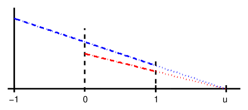
Figure 2. Exponents $0\leq\kappa\leq 1$ in $\|f_{\alpha}^{\delta}-f^{\dagger}\|_{\mathcal{X}_{r}}=O(\delta^{\kappa})$ as $\delta~{}\to~{}0$ corresponding to Theorem 2.1 for data smoothing problem with different parameters $a=1$, $\gamma=1$ (blue) and $a=0$, $\gamma=1/2$ (red, dashed).

As can be seen from the plot, the interpolation estimate used to derive the Hölder stability condition (6.2) from the Lipschitz estimate (6.1) is suboptimal when $s<u$. In addition, also the range of admissible smoothness indices $s\leq u\leq 2s+a$ shrinks when increasing $a$. A general guideline for the choice of parameters $a$ and $\gamma$ in the stability condition (A2) is therefore to choose these parameters as large as possible. The parameter $s$ in the regularization terms should also be chosen as large as possible, but small enough, such that $x^{\dagger}\in\mathcal{X}_{u}$ can be expected for some $u\geq s$.

6.2. Parameter identification

The parameter identification problem discussed in Section 5.2 can be phrased as $F(c)=U^{\delta}$ with $F(c)=U$ where $U$ solves

(6.3) $$U^{\prime}(t)+c(t)U(t)=0,\qquad U(0)\neq 0\quad\text{given}.$$

We set $X_{0}=L^{2}(0,T)$ with norm $\|c\|_{0}^{2}=\int_{0}^{T}c(s)^{2}ds$ and and $X_{2}=H^{2}(0,T)$ with norm $\|c\|_{2}^{2}=\|c\|^{2}_{0}+\|c^{\prime\prime}\|_{0}^{2}$. For any parameter $0\leq s\leq 2$, we then obtain by interpolation that $X_{s}=H^{s}(0,T)$. As shown in the previous section, we have

$$\|c_{1}-c_{2}\|_{L^{2}(0,T)} \leq R(\rho)\|F(c_{1})-F(c_{2})\|_{L^{2}(0,T)}^{\frac{s}{s+1}}$$

here for all $c_{1},c_{2}\in H^{s}(0,T)$ with $c_{i}\geq 0$ and $\|c_{1}\|_{H^{s}(0,T)},\|c_{2}\|_{H^{s}(0,T)}\leq\rho$ and with appropriate function $R(\rho)$. In our tests, we will set $s=1$ or $s=2$.

The evaluation of $F$ requires the solution of the initial value problem (6.3). For this we approximate $U$ by continuous piecewise linear functions over a regular grid of $[0,T]$, and we represent $c$ by cubic splines over the same grid. The problem (6.3) is then solved by a Petrov-Galerkin method using discontinuous piecewise constant test functions. This allows us to exactly evaluate the derivative $W=F^{\prime}(c)h$ and the adjoint $d=F^{\prime}(c)^{*}r$ on the discrete level. For the computation of approximate minimizers for the Tikhonov functional, we then utilize a Gauß-Newton method.

To evaluate the convergence behavior of our regularization strategy, we again consider three reference solutions of different smoothness, defined by

$$c^{\dagger}(t)=\begin{cases}t,&t<T/2,\\ T-t,&t>T/2,\end{cases}\qquad c^{\dagger}(t)=t\sqrt{t},\qquad\text{and}\qquad c^{\dagger}(t)=t(T-t).$$

Here $c^{\dagger}\in\mathcal{X}_{u}$ for all $u<3/2$ in the first case and $c^{\dagger}\in\mathcal{X}_{u}$ for all $u<2$ in the second. Note that we only have $c^{\dagger}\in\mathcal{X}_{u}$ for all $u<5/2$ in the third case, since $X_{s}\neq H^{s}(0,T)$ for $s>5/2$ due to the appearance of additional boundary conditions; see [12] for details. The convergence rates of Theorem 2.1 are listed in Table 5.

	$s=1$			$s=2$
$u$	$\alpha$	$\|c_{\alpha}^{\delta}-c^{\dagger}\|_{\mathcal{X}_{0}}$	$\|c_{\alpha}^{\delta}-c^{\dagger}\|_{\mathcal{X}_{1}}$	$\alpha$	$\|c_{\alpha}^{\delta}-c^{\dagger}\|_{\mathcal{X}_{0}}$	$\|c_{\alpha}^{\delta}-c^{\dagger}\|_{\mathcal{X}_{1}}$
$\frac{3}{2}$	$\delta^{5/3}$	$\delta^{1/2}$	$\delta^{1/6}$	$\delta^{22/9}$	—	—
$2$	$\delta^{3/2}$	$\delta^{1/2}$	$\delta^{1/4}$	$\delta^{2}$	$\delta^{2/3}$	$\delta^{1/3}$
$\frac{5}{2}$	$\color[rgb]{0,0,1}\delta^{7/5}$	$\color[rgb]{0,0,1}\delta^{1/2}$	$\color[rgb]{0,0,1}\delta^{3/10}$	$\delta^{26/15}$	$\delta^{2/3}$	$\delta^{2/5}$

Table 5. Parameter choice and convergence estimates of Theorem 2.1 for the parameter identification problem using the stability condition (A2) with $a=0$ and $\gamma=s/(s+1)$. Results in blue are not covered since $s\leq u\leq 2s+a$ or $-a\leq r\leq s$ is violated.

In Table 6 we list the reconstruction errors obtained in our numerical tests with a-posteriori parameter choice strategy according to Theorem 2.2.

	$s=1$			$s=2$
$u$	$\alpha$	$\|f_{\alpha}^{\delta}-f^{\dagger}\|_{\mathcal{X}_{0}}$	$\|f_{\alpha}^{\delta}-f^{\dagger}\|_{\mathcal{X}_{1}}$	$\alpha$	$\|f_{\alpha}^{\delta}-f^{\dagger}\|_{\mathcal{X}_{0}}$	$\|f_{\alpha}^{\delta}-f^{\dagger}\|_{\mathcal{X}_{1}}$
$\frac{3}{2}$	$\delta^{1.44}$	$\delta^{0.52}$	$\delta^{0.17}$	$\delta^{2.34}$	$\color[rgb]{0,0,1}\delta^{0.64}$	$\color[rgb]{0,0,1}\delta^{0.22}$
$2$	$\delta^{1.46}$	$\delta^{0.54}$	$\delta^{0.18}$	$\delta^{2.04}$	$\delta^{0.72}$	$\delta^{0.37}$
$\frac{5}{2}$	$\color[rgb]{0,0,1}\delta^{1.56}$	$\color[rgb]{0,0,1}\delta^{0.57}$	$\color[rgb]{0,0,1}\delta^{0.19}$	$\delta^{1.65}$	$\delta^{0.69}$	$\delta^{0.41}$

Table 6. Parameter choice and reconstruction errors for data smoothing problem using (A2) with $a=1$ and $\gamma=1$ and a-posteriori parameter choice. Results in blue are not covered by theory since one of the conditions $s\leq u\leq 2s+a$ or $-a\leq r\leq s$ is violated.

Again, the results are in very good agreement with the theoretical predictions displayed in Table 5. Similar results were also obtained for the a-priori parameter choice but they are omitted here.

7. Discussion

In this paper, we investigated Tikhonov regularization in Hilbert scales under a conditional stability assumption for the considered inverse problem. Optimal convergence rates were established for a-priori and a-posteriori parameter choice strategies. Apart from the conditional stability estimate, no further assumptions on the continuity or differentiability of the operator $F$ were required.

For the statement of our main results, we utilized here the framework of Hilbert scales. This allowed us to keep the presentation compact and to discuss in detail the relation to previous work. An extension of the analysis to Banach scales seems to be possible and will be a topic of future research.

Conditional stability estimates have been used recently for the convergence analysis of Landweber iteration [3]. It has been observed there that a Hölder stability condition (A2) with $\gamma>1/2$ together with the usual continuity assumptions already implies the tangential cone condition. Stability conditions for linear or linearized problems have also been used for the convergence analysis of iterative regularization methods in Hilbert scales; see e.g. [4, 14]. An extension of such a convergence analysis under weaker Hölder stability conditions, which have been utilized in this paper, may be possible and should also be addressed in the future.

References

• [1] J. Cheng, B. Hofmann, and S. Lu. The index function and Tikhonov regularization for ill-posed problems. J. Comput. Appl. Math., 265:110–119, 2014.
• [2] J. Cheng and M. Yamamoto. On new strategy for a priori choice of regularizing parameters in Tikhonov’s regularization. Inverse Problems, 16:L31–L38, 2000.
• [3] M. V. de Hoop, L. Qiu, and O. Scherzer. Local analysis of inverse problems: Hölder stability and iterative reconstruction. Inverse Problems, 28:045001, 2012.
• [4] H. Egger. Fast fully iterative Newton-type methods for inverse problems. J. Inv. Ill-posed Problems, 15:257–276, 2007.
• [5] H. Egger. Regularization of inverse problems with large noise. J. Phys. Conf. Ser., 124:012022, 2008.
• [6] H. W. Engl, M. Hanke, and A. Neubauer. Regularization of Inverse Problems, volume 375 of Mathematics and its Applications. Kluwer Academic Publishers Group, Dordrecht, 1996.
• [7] B. Hofmann and P. Mathé. Tikhonov regularization with oversmoothing penalty for non-linear ill-posed problems in Hilbert scales. Inverse Problems, 34:015007, 14, 2018.
• [8] B. Hofmann and R. Plato. On ill-posedness concepts, stable solvability and saturation. J. Inverse Ill-Posed Probl., 26:287–297, 2018.
• [9] B. Hofmann and M. Yamamoto. On the interplay of source conditions and variational inequalities for nonlinear ill-posed problems. Appl. Anal., 89:1705–1727, 2010.
• [10] V. A. Morozov. Methods for Solving Incorrectly Posed Problems. Springer-Verlag, New York, 1984.
• [11] F. Natterer. Error bounds for Tikhonov regularization in Hilbert scales. Appl. Anal., 18:29–37, 1984.
• [12] A. Neubauer. When do Sobolev spaces form a Hilbert scale? Proc. Amer. Math. Soc., 103:557–562, 1988.
• [13] A. Neubauer. Tikhonov regularization of nonlinear ill-posed problems in Hilbert scales. Appl. Anal., 46:59–72, 1992.
• [14] A. Neubauer. On Landweber iteration for nonlinear ill-posed problems in Hilbert scales. Numer. Math., 85:309–328, 2000.
• [15] U. Tautenhahn. Error estimates for regularized solutions of nonlinear ill-posed problems. Inverse Problems, 10:485–500, 1994.