Choice of the Parameters in A Primal-Dual Algorithm for Bregman Iterated Variational Regularization

Abstract

Focus of this work is solving a non-smooth constraint minimization problem by a primal-dual splitting algorithm involving proximity operators. The problem is penalized by the Bregman divergence associated with the non-smooth total variation (TV) functional.

We analyse two aspects: Firstly, the convergence of the regularized solution of the minimization problem to the minimum norm solution. Second, the convergence of the iteratively regularized minimizer to the minimum norm solution by a primal-dual algorithm. For both aspects, we use the assumption of a variational source condition (VSC). This work emphasizes the impact of the choice of the parameters in stabilization of a primal-dual algorithm. Rates of convergence are obtained in terms of some concave, positive definite index function.

The algorithm is applied to a simple two dimensional image processing problem. Sufficient error analysis profiles are provided based on the size of the forward operator and the noise level in the measurement.

Keywords: iterative regularization, primal dual algorithm, Bregman distance, total variation, proximal mapping

footnote

1 Introduction

One can only stabilize an algorithm for correctly defined parameters. Otherwise, no regularization technique provides approximate solution for an inverse ill-posed problem. This work does not only focus on stability analysis of a convex optimization algorithm, but it also introduces the algorithm as an iterative regularization procedure. The algorithm we take up is in the generalization of gradient descent by means of proximal mapping. In the study of convergence of a gradient descent algorithm, it is known that the stability of the algorithm is in fact based on how the step-length is defined, e.g. [10]. By stability, we mean convergence of the iterative solution to the minimizer of some appropriately defined objective functional. However, from regularization point of view, this is an insufficient stability analysis for the study of inverse ill-posed problems aims to provide answer for real life application problems. Therefore, in order to fill this gap in the context of variational regularization, this work aims to go further than just defining a step-length for the stability of a convex optimization algorithm.

In general terms, regularization theory deals with the approximation of some ill-posed inverse problems by a family of parametrized well-posed problems. Traditional quadratic-Tikhonov regularization [57, 58] has been well established and analyzed [31]. As an alternative to classical Tikhonov regularization, convex variational regularization with some general penalty functional has gained interest over the last decade. Analysis of convex variational regularization has been motivated by a new image denoising method called “total variation“ [51]. Further studies of the method have been widely carried out in the communities of inverse problems and optimization [1, 7, 9, 21, 22, 23, 29, 30, 60].

Recently proposed non-smooth penalty terms have risen the interest in the study of variational regularization. Convexity of the objective functional is the most essential property to analyze the stability of the regularized solution of the inverse problem, or equivalently the minimization problem. Formulating the minimization problem as variational problem and estimating convergence rates under the assumption that the minimum norm solution satisfies a type of variational source condition (VSC) has been well established, [18, 35, 36, 37, 38, 46]. In addition to the estimation of the convergence rates, verification of VSC has also become popular, see [40, 42, 55]. A recent study on the existence of the VSCs for linear or non-linear problems can be found in [32].

When obtaining the stable regularized solution, it is also important that this solution meets the constraints of the inverse problems. These contraints are defined mostly due to the physical facts of the solution. Therefore, the necessity of solving a constrained minimization problem is well understood. We are tasked with approximating the solution of some constrained minimization problem by an efficient proximal gradient algorithm as an iterative regularization method.

Inverse problems arise in many scientific fields: X-ray computed tomography, image processing, signal processing, wave scattering, shape reconstruction, etc. We must emphasize that although many problems lie in the same family of inverse problems, each problem may differ from each other depending on their physical or engineering facts. The properties of the targeted data and the forward operator that we define in the following section are suitable for tomographic reconstruction problems.

2 Notations and Mathematical Setting

Over the finite dimensional Hilbert spaces $\mathcal{X}=\mathbb{R}^{N}$ and $\mathcal{Y}=\mathbb{R}^{M}$, let us assume some linear, injective, forward operator $T:\mathcal{X}\rightarrow\mathcal{Y}.$ We consider the following linear ill-posed problem

$$\delta\xi+Tu=v^{\delta},$$ (2.1)

where the given noisy data $v^{\delta}\in\mathcal{Y}$ and the noise model $\xi$ with the noise magnitude $\delta.$ Furthermore, we also impose non-negativity constraint on our targeted data $u.$ Then, the constraint domain $\Omega:=\{u\in\mathcal{X}:u_{i}\geq 0\mbox{ for each }i=1,\cdots,N\},$ is treated as the indicator function, [16], that is defined by

$$h(u)=1_{\Omega}(u):=\left\{\begin{array}[]{rcl}0&\mbox{, for}&u\in\Omega\subset\mathcal{X}\\ \infty&\mbox{, for}&u\notin\Omega\subset\mathcal{X}.\end{array}\right.$$ (2.4)

Throughout the work, unless otherwise stated, the notation $\|\cdot\|$ without any subscript will be used to denote the usual Euclidean norm. Let $\sigma(T^{\ast}T):=\{\sigma_{1},\sigma_{2},\cdots\sigma_{M}\}$ be the spectrum of $T^{\ast}T.$ Then, for the finite dimensional forward operator $T:\mathbb{R}^{N}\rightarrow\mathbb{R}^{M}$ where $M<N,$ we define

$$\|T\|:=\max_{1\leq k\leq M}\left\{\sqrt{\sigma_{k}}\right\}.$$

Regarding the stability analysis for the algorithm, we will refer to one fundamental equality that has been also given in [56, Eq. (2.1)]. For some $u_{1},u_{2}\in\mathcal{X}$ and $\rho\in\mathbb{R},$ the following equality holds,

$$\|\rho u_{1}+(1-\rho)u_{2}\|^{2}=\rho\|u_{1}\|^{2}+(1-\rho)\|u_{2}\|^{2}-\rho(1-\rho)\|u_{1}-u_{2}\|^{2}.$$ (2.5)

For some real valued and convex function $f:\mathcal{X}\rightarrow\mathcal{X}$ and some point $x$ in the domain of $f,$ the subdifferential of $f$ at $x^{\prime},$ denotes $\partial f(x^{\prime})$ is defined by

$$\partial f(x^{\prime}):=\left\{\eta\in\mathcal{X}^{\ast}:f(x)-f(x^{\prime})\geq\langle\eta,x-x^{\prime}\rangle\mbox{ for all }x\in\mathcal{X}\right\}.$$ (2.6)

Definition 2.1.

[Generalized Bregman Distance] Let $\mathcal{J}:\mathcal{X}\rightarrow\mathbb{R}_{+}\cup\{\infty\}$ be a convex functional with the subgradient $q^{\ast}\in\partial\mathcal{J}(u^{\ast}).$ Then, for $u,u^{\ast}\in\mathcal{X},$ the Bregman distance associated with the functional $\mathcal{J}$ is defined by

$$D_{\mathcal{J}}: \mathcal{X}\times\mathcal{X} \longrightarrow\mathbb{R}_{+}$$ (2.7)

$$(u,u^{\ast}) \longmapsto D_{\mathcal{J}}(u,u^{\ast}):=\mathcal{J}(u)-\mathcal{J}(u^{\ast})-\langle q^{\ast},u-u^{\ast}\rangle.$$

It is well known that the Bregman distance does not satisfy symmetry,

$$D_{\mathcal{J}}(u,u^{\ast})\neq D_{\mathcal{J}}(u^{\ast},u),$$

and for the defined convex functional $\mathcal{J},$

$$D_{\mathcal{J}}(u,u^{\ast})\geq 0.$$

Over the past decades, variational and traditional regularization strategies have been dedicated to find the stable minimum of the generalized form of the Tikhonov functional

$$H_{\alpha}: \mathcal{X} \times\mathcal{Y}\longrightarrow\mathbb{R}_{+}$$ (2.8)

$$(u ,v^{\delta})\longmapsto H_{\alpha}(u,v^{\delta}):=\frac{1}{2\alpha}\|Tu-v^{\delta}\|^{2}+\mathcal{J}(u),$$

with a convex, lower-semicontinuous, not necessarily smooth penalty functional $\mathcal{J}:\mathcal{X}\longrightarrow\mathbb{R}_{+}\cup\{\infty\}$ and a regularization parameter $\alpha>0.$ On the other hand, we consider the following objective functional,

$$F_{\alpha}: \mathcal{X} \times\mathcal{Y}\longrightarrow\mathbb{R}_{+}$$ (2.9)

$$(u ,v^{\delta})\longmapsto F_{\alpha}(u,v^{\delta}):=\frac{1}{2}\|Tu-v^{\delta}\|^{2}+\alpha D_{\mathcal{J}}(u,u^{0})+h(u),$$

with some initial estimation $u^{0}\in\mathcal{X},$ where we have included the indicator of the positive orthant. In particular, we associate the Bregman distance penalty term with the total variation (TV) functional defined by

$$TV(u,\Omega)=\mathcal{J}(u):=\int_{\Omega}|\nabla u(x)|dx\approxeq\sum_{i}|\nabla_{i}u|,$$ (2.10)

which is, in the 3D case, $i=(i_{x},i_{y},i_{z}).$ For some $u_{1},u_{2}$ in the domain of $T,$ from Lipschitz continuity of the misfit term $\frac{1}{2}\|Tu-v^{\delta}\|^{2}$ that is,

$$\|T^{T}T(u_{1}-u_{2})\|^{2} \leq \|T\|^{2}\|T(u_{1}-u_{2})\|^{2}$$

$$= \|T\|^{2}\langle T(u_{1}-u_{2}),T(u_{1}-u_{2})\rangle$$

$$= \|T\|^{2}\langle T^{T}T(u_{1}-u_{2}),u_{1}-u_{2}\rangle,$$

one can easily observe the following,

$$-\langle u_{1}-u_{2},T^{T}T(u_{1}-u_{2})\rangle\leq-\frac{1}{\|T\|^{2}}\|T^{T}T(u_{1}-u_{2})\|^{2}.$$ (2.11)

For the sake of following further calculations easily in future developments of this work, we introduce TV in the composite form

$$J(u)=g(Du)\mbox{ where, }g(\cdot)=\|\cdot\|_{1}\mbox{ with }D(\cdot)=\nabla(\cdot).$$ (2.12)

Thus,

$$\partial J(u)=D^{\ast}\partial g(Du).$$ (2.13)

Total variation type regularization targets the reconstruction of bounded variation (BV) class of vectors, which are functions in the infinite dimensional mathematical setting, that are defined by

$$BV(\Omega):=\{u\in\ell^{1}(\Omega):TV(u,\Omega)<\infty\}$$ (2.14)

with the norm

$$\|\varphi\|_{BV}:=\|u\|_{1}+TV(u,\Omega).$$ (2.15)

Let the mean value $MV:\ell^{1}(\Omega)\rightarrow\mathbb{R}$ be defined by

$$MV[u]:=\frac{1}{|\Omega|}\int_{\Omega}u(x)dx.$$ (2.16)

It has been stated in [1, Eq. (4.3)] that, over the bounded domain $\Omega,$ for any $u\in BV(\Omega)$ has the following decomposition

$$u=\tilde{u}+MV[u]\vec{1},$$ (2.17)

where

$$MV[\tilde{u}]=0.$$ (2.18)

3 Discussion of Previous Works and Contribution

In an early study [49], Bregman iteration has been proposed to solve the basis pursuit problem. Therein, it has been numerically demonstrated that the efficiency of the algorithms gets improved with the inclusion of the Bregman distance playing the role of penalty term in the objective functional $F_{\alpha}$ in (2.9). In a recent study by Sprung and Hohage et al., 2017, [55], it has been stated that minimizing the objective functionals in the form of (2.8) can be interpreted as proximal point methods when one considers the penalty term as a quadratic function. Applying optimization algorithms in the field of inverse problems as iterative regularization method has become popular. Authors in [34] have proposed some primal-dual algorithm, wherein the convergence has been studied for the given noiseless measurement data. Different forms of nested primal-dual algorithms for solving proximal mappings have been introduced in [24].

We consider linear, inverse ill-posed problems in the general form (2.1) and study the stability of both iterative and non-iteartive regularized solutions in the context of convex variational regularization. The main results of our work are derived in the presence of noisy measurements and specifically address convex variational regularization. From the subdifferential characterization of the regularized minimizer for the functional (2.9), a new iterative regularization algorithm shall be developed. In Section 7, stability analysis of the iteratively regularized solution is analyzed in the Hadamard sense.

4 Overview of the Fundamentals of the Regularization Theory

We split this section into three subsections. Section 4.1 reviews the regularization theory in the continuous sense. This part will be used to analyse the convergence of the regularized minimum $u_{\alpha}^{\delta}$ towards the minimum norm solution $u^{\dagger}.$ A choice of the regularization parameter which is a-posteriori obeying Morozov‘s dicrepancy principle is introduced in the following up sections. Section 4.4, on the other hand, reviews the iterative regularization theory which will be used for showing the convergence of the iteratively regularized minimum $u_{i+1}$ still towards the minimum norm solution $u^{\dagger}.$

4.1 Continuous regularization

In the Banach space setting, the concept of $\mathcal{J}$-minimizing solution is well known for the functionals in the form of (2.8), see e.g.,[53, Lemma 3.3], [32]. In our case, since Bregman distance is associated with the TV functional, we have

$$Tu^{\dagger}=v^{\dagger}\mbox{ and }\|u^{\dagger}\|=\min\{\|u\|:u\in\mathrm{BV}(\Omega),Tu=v^{\dagger}\}.$$ (4.1)

According to our mathematical setting, the functional $\mathcal{J}:\Omega\subset\mathcal{X}\rightarrow\mathbb{R}_{+}$ attains some finite value only at some finite point $u\in\mathrm{BV}(\Omega),$ [32, Assumption 1.1 (i)]. Moreover, our linear forward operator is defined on a uniformly convex Banach space [53, Theorem 2.53(k) & Lemma 3.3]. In case of $u^{0}$ to be constant, then from our setting above (2.12) and (2.13), our notation in (4.1) boils down to its conventional form named $\mathcal{J}$-minimizing solution. In what follows, the minimum norm solution that has just been introduced by (4.1) will be denoted by $u^{\dagger}.$

Briefly speaking, establishing convergence result for some regularization method in the Hadamard sense begins with seeking to approximate the true solution by a family of regularized solutions of the problem

$$u_{\alpha}^{\delta}\in{\rm arg\,min}_{u\in\mathcal{X}}F_{\alpha},$$ (4.2)

satisfying the following properties:

1. For any $v^{\delta}\in\mathcal{Y}$ there exists a solution $u_{\alpha}^{\delta}\in\mathcal{X}$ to the problem (4.2);

2. For any $v^{\delta}\in\mathcal{Y}$ there is no more than one $u_{\alpha}^{\delta}\in\mathcal{X};$

3. Convergence of the regularized solution $u_{\alpha}^{\delta}$ to the minimum norm solution $u^{\dagger}$ must continuously depend on the given data $v^{\delta}$, i.e.

   $$\|u_{\alpha}^{\delta}-u^{\dagger}\|\rightarrow 0\mbox{ as }\alpha=\alpha(\delta,v^{\delta})\rightarrow 0\mbox{ for }\delta\rightarrow 0$$

   whilst

   $$\|v^{\dagger}-v^{\delta}\|\leq\delta$$

   where $v^{\dagger}\in\mathcal{R}(T)\subset\mathcal{Y}$ is the noiseless measurement and $\delta$ is the noise level.

Existence and uniqueness of the regularized minimizer for the functional (2.9) is ensured by the following facts: Bregman distance is convex and lower semi-continuous in its first term, and so is the indicator function. In (iii) it is stated that when the given measurement $v^{\delta}$ lies in some $\delta-$ball centered at the noisless measurement $v^{\dagger}$, i.e. $v^{\delta}\in\mathcal{B}_{\delta}(v^{\dagger}),$ then the regularized solution $u_{\alpha}^{\delta}$ must converge to the minimum norm solution of the inverse problem $u^{\dagger}$ as the regularization parameter $\alpha(\delta,v^{\delta})$ decays sufficiently, see [31, Section 2, Properties (2.1) - (2.3)]. The main results of this work are dedicated to justify the condition ‘(iii)’ with the inclusion of the noisy measurement $v^{\delta}.$

It is well known that some regularization operator can be defined explicitly for the objective functionals in the form of (2.8) with $\mathcal{J}(\cdot)=\frac{1}{2}\|\cdot\|^{2},$ [31, Definition 3.1]. This is not the case anymore in the variational regularization strategy due to the non-smoothness of the penalty term $\mathcal{J}$. However, a regularization procedure definition can still be given fulfilling Hadamard‘s principle. Depending on the asymptotics of the regularization parameter $\alpha,$

$$\alpha(\delta,v^{\delta})\rightarrow 0\mbox{ and }\frac{\delta^{2}}{\alpha(\delta,v^{\delta})}\rightarrow 0\mbox{, as }\delta\rightarrow 0,$$ (4.3)

regularization theory is concerned with the error estimation for the difference between the approximately regularized solution $u_{\alpha}^{\delta}$ and minimum norm solution $u^{\dagger}$ of the inverse problem (2.1) as defined before.

Iterative regularization methods aim to produce stable approximate solutions to the problem (4.2) throughout some iterative procedure, e.g., with the focus on minimizing the discrepancy $\|Tu-v^{\delta}\|$ by producing a sequence of iterates $\hat{u}_{i}.$ Usually the iteration is terminated at the iteration step $N$ by the choice of some stopping criterion, which is a-posteriori $N=N(v^{\delta},\delta).$ This work concerns with the choice of the regularization parameter not only in the continuous sense i.e., $\alpha=\alpha(v^{\delta},\delta),$ but also within the iterative procedure i.e., $\alpha_{n}=\alpha_{n}(v^{\delta},\delta).$ The scientific notion behind these notations can be reviewed in [53, pp. 63]. The following definition is a quick adaptation of [53, Definition 3.20] for our mathematical setting and furthermore suits our iterative regularization scheme which shall be introduced in Section 7.1.

Therefore, we will investigate the stability of the iterative procedure as the number of the iterative steps tend to infinity. In this work, the iterative regularization procedure involves proximal mappings.

Definition 4.1.

[Proximal mapping] Let $\mathcal{J}:\mathbb{R}^{N}\rightarrow\mathbb{R}\cup\{\infty\}$ be a proper, convex, lower-semicontinious function. Then $\mathrm{prox}_{\mathcal{J}}$ is defined as the unique minimizer

$$\mathrm{prox}_{\mathcal{J}}(\tilde{u}):={\rm arg\,min}_{u\in\mathbb{R}^{N}}\mathcal{J}(u)+\frac{1}{2}\|u-\tilde{u}\|^{2}.$$

4.2 Smoothness of the minimum norm solution under variational inequalities

Measuring the deviation of the regularized solution $u_{\alpha}^{\delta}$ from the minimum norm solution by a-priori and a-posteriori strategies for the choice of the regularization parameter in Banach spaces with the VSC has been widely studied [12], [32], [35], [39, Eq. (1.4)], [44, Section 4] [53, Theorem 2.60 - (g), Subsection 3.2.4]. The objective is to bound the total error estimation function defined, for some coefficient $\Lambda\in\mathbb{R}_{+}$ depending on the functional properties of $\mathcal{J}$ and its domain, by

$$E: \mathcal{X}\times\mathcal{X} \longrightarrow\mathbb{R}_{+}$$ (4.4)

$$(u_{\alpha}^{\delta},u^{\dagger}) \longrightarrow E(u_{\alpha}^{\delta},u^{\dagger}):=\Lambda\|u_{\alpha}^{\delta}-u^{\dagger}\|.$$

Different forms of the VSC have been considered for establishing convergence and convergence rates results. A recent and concise work on the verification of the VSCs in general terms has been studied by Flemming et.al., 2018 [32].

Our work does not focus on verification of the VSC. However, by using fundamental functional analysis, it is still possible to give mathematical motivation for the formulation of our VSC. First, according to the Poincaré-Wirtinger inequality, see [13, Theorem 3.1], for some $u\in\mathrm{BV}(\Omega),$ there exists some constant $C_{\Omega}$ such that

$$\|\nabla u\|_{1}\geq\frac{1}{C_{\Omega}}\|u-\mathrm{MV}[u]\vec{1}\|_{1}$$

holds. Addition to the fundamental inequality, the early established result in [2, Eq. (3.43)] and equivalence of the norm in the finite dimensional setting, lead to

$$\|\nabla u\|_{1}\geq\frac{1}{C_{\Omega}}\|u-\mathrm{MV}[u]\vec{1}\|_{1}\geq\frac{1}{2}\|u\|_{1}\geq\frac{1}{2}\|u\|_{2}.$$

With that being stated, VSC could rather be formulated as a direct estimator for the total error functional (4.4).

Assumption 4.2.

[Variational Source Condition] Let $T:\mathcal{X}\rightarrow\mathcal{Y}$ be linear, injective forward operator and $v^{\dagger}\in\mathrm{range}(T).$ There exists some constant $\sigma\equiv\sigma(C_{\Omega})\in(0,1]$ and a concave, monotonically increasing index function $\Psi$ with $\Psi(0)=0$ and $\Psi:[0,\infty)\rightarrow[0,\infty)$ such that for $q^{\dagger}\in\partial\mathcal{J}(u^{\dagger})$ the minimum norm solution $u^{\dagger}\in\mathrm{BV}(\Omega)$ satisfies

$$\sigma\|u-u^{\dagger}\|\leq\mathcal{J}(u)-\mathcal{J}(u^{\dagger})+\Psi\left(\|Tu-Tu^{\dagger}\|\right)\mbox{, for all }u\in\mathcal{X}.$$ (4.5)

Above, the estimation of the coefficient function $\sigma$ is an open question to be answered under the consideration of $\mathcal{J}=TV.$

In some works, the Bregman distance itself is directly taken as the estimator for the total error functional (4.4) and VSC is formulated as an upper bound for the Bregman distance, see e.g. [39]. The reader can find our further convergence result based on this formulation of the VSC in the Appendix A.

One straightforward conclusion of VSC follows from non-negativity of the total error functional (4.4),

$$\mathcal{J}(u^{\dagger})-\mathcal{J}(u)\leq\Psi\left(\|Tu-Tu^{\dagger}\|\right),$$ (4.6)

for all $u\in\mathcal{X}.$ We furthermore state one fundamental idendity that is valid for the concave functions, see [39, Proposition 1], [53, Eq. (4.37)],

$$\Psi(K\delta)\leq K\Psi(\delta),\mbox{ for }K\geq 1.$$ (4.7)

We will develop convergence rates results from two different aspects. Firstly, the convergence of the non-iterative regularized solution $u_{\alpha}^{\delta}$ of the problem (4.2) towards the minimum norm solution $u^{\dagger}.$ We conduct this analysis in the continuous setting. Secondly, we study the convergence of the iteratively regularized solution $\hat{u}_{\alpha_{i}}^{\delta},$ where $i=1,2,\cdots$ indicate the iteration step, produced by some primal-dual algorithm still towards the minimum norm solution $u^{\dagger}.$ In both investigations, the convergence rates will be expressed in terms of the index function $\Psi$ and be achieved by a-posteriori choice of the regularization parameter $\alpha$ , see Section 4.3 for the details.

4.3 Choice of the Regularization Parameter: Morozov’s Discrepancy Principle

We are concerned with asymptotic properties of the regularization parameter $\alpha$ for the Tikhonov-regularized solution obtained by Morozov’s discrepancy principle (MDP). MDP serves as an a posteriori parameter choice rule for the Tikhonov type objective functionals (2.9) and has certain impact on stabilizing the total error functional $E$ having the assumed relation (1.1). As has been introduced in [5, Theorem 3.10] and [6], we use the following set notations in the theorem formulations that are necessary to establish the error estimation between the regularized solution $u_{\alpha}^{\delta}$ for the problem (4.2) and the minimum norm solution $u^{\dagger},$

$$\overline{S} := \left\{\alpha:\|Tu_{\alpha}^{\delta}-v^{\delta}\|\leq\overline{\tau}\delta\mbox{ for }u_{\alpha}^{\delta}={\rm arg\,min}_{u\in\mathcal{X}}\{F_{\alpha}(u,v^{\delta})\}\right\},$$ (4.8)

$$\underline{S} := \left\{\alpha:\underline{\tau}\delta\leq\|Tu_{\alpha}^{\delta}-v^{\delta}\|\mbox{ for }u_{\alpha}^{\delta}={\rm arg\,min}_{u\in\mathcal{X}}\{F_{\alpha}(u,v^{\delta})\}\right\},$$ (4.9)

where the discrepancy set radii $1<\underline{\tau}\leq\overline{\tau}<\infty$ are fixed. Analogously, also as well known from [31, Eq. (4.57) and (4.58)] and [45, Definition 2.3], we are interested in such a regularization parameter $\alpha(\delta,v^{\delta}),$ with some fixed discrepancy set radii $1<\underline{\tau}\leq\overline{\tau}<\infty,$ that

$$\alpha(\delta,v^{\delta})\in\{\alpha>0\mbox{ }|\mbox{ }\underline{\tau}\delta\leq\|Tu_{\alpha}^{\delta}-v^{\delta}\|\leq\overline{\tau}\delta\}=\overline{S}\cap\underline{S}\mbox{ for the given }(\delta,v^{\delta}).$$ (4.10)

It is also the immediate consequences of MDP that the following estimations

$$\|Tu_{\alpha}^{\delta}-Tu^{\dagger}\|\leq(\overline{\tau}+1)\delta,$$ (4.11)

$$(\underline{\tau}-1)\delta\leq\|Tu_{\alpha}^{\delta}-Tu^{\dagger}\|,$$ (4.12)

hold true.

4.4 Iterative regularization

By an iterative procedure involving some iteration operator $R_{I},$ [11, Ch. 6], we aim to construct some approximation to the given inverse ill-posed problem (2.1)

$$u_{i}=R_{I}(v^{\delta},w_{i-1},\Gamma),$$ (4.13)

where $w^{i-1}$ is the collection of dual variables used during $i-1$ iteration steps, and $\Gamma$ is the auxiliary parameters such as step-size, relaxation parameter, regularization parameter.

In the iterative regularization procedures, discrepancy principles act as the stopping rules for the corresponding algorithms, [11, Section 6].

Definition 4.3.

[Morozov‘s Discrepancy Principle (MDP), [11, Def. 6.1]]

Given deterministic noise model $\|v^{\dagger}-v^{\delta}\|\leq\delta,$ if we choose $\tau>1$ and $i^{\ast}=i^{\ast}(\delta,v^{\delta})$ such that

$$\|Tu_{i^{\ast}}-v^{\delta}\|\leq\tau\delta<\|Tu_{i}-v^{\delta}\|$$ (4.14)

is satisfied for $u_{i^{\ast}}=R_{I}(v^{\delta},w_{i^{\ast}-1},\vec{\alpha})$ and $u_{i}=R_{I}(v^{\delta},w_{i-1},\vec{\alpha})$ for all $i<i^{\ast},$ then $u_{i^{\ast}}$ is said to satisfy Morozov‘s discrepancy principle.

Following up MDP, some immediate consequences can be given below,

$$\|Tu_{i^{\ast}}^{\delta}-Tu^{\dagger}\|\leq(\tau+1)\delta,$$ (4.15)

likewise,

$$\tau\delta\leq\|Tu_{i}-v^{\delta}\| \Rightarrow \tau\delta\leq\|Tu_{i}-Tu^{\dagger}\|+\delta$$ (4.16)

$$\Rightarrow (\tau-1)\delta\leq\|Tu_{i}-Tu^{\dagger}\|$$

$$\Rightarrow (\tau-1)^{2}\delta^{2}\leq\|Tu_{i}-Tu^{\dagger}\|^{2}$$

$$\Rightarrow -\|Tu_{i}-Tu^{\dagger}\|^{2}\leq-(\tau-1)^{2}\delta^{2}.$$

5 Subgradient Characterization of the Regularized Solution $u_{\alpha}^{\delta}$: Primal-Dual Splitting

Still in the continuous setting, the subgradient characterization of the regularized solution $u_{\alpha}^{\delta}$ of the problem (4.2) is to be studied. Our iterative regularization algorithm will arise from characterization of the primal and the dual solutions. This characterization will form some coupled system which makes the primal solution depend on the dual one, and vice versa. Before moving on to the characterization, let us introduce some more notations. Since $u_{\alpha}^{\delta}$ is the minimizer of the objective functional (2.9), then by the first order optimality condition

$$0\in\partial F_{\alpha}(u_{\alpha}^{\delta},v^{\delta}),$$

which implies,

$$0=\frac{1}{\alpha}T^{T}(Tu_{\alpha}^{\delta}-v^{\delta})+\partial\mathcal{J}(u_{\alpha}^{\delta})-\partial\mathcal{J}(u^{0})+\hat{z}\mbox{, where }\hat{z}\in\partial h(u_{\alpha}^{\delta}).$$ (5.1)

Furthermore, recall the settings in (2.12) and (2.13) to represent (5.1) in the following form

$$0=\frac{1}{\alpha}T^{T}(Tu_{\alpha}^{\delta}-v^{\delta})+D^{T}\hat{w}_{\alpha}^{\delta}-D^{T}\hat{w}^{0}+\hat{z},$$

where $\hat{w}_{\alpha}^{\delta}\in\partial g(Du_{\alpha}^{\delta})$ and likewise $\hat{w}^{0}\in\partial g(Du^{0}),$ and we recall that $g(\cdot)=\|\cdot\|.$ Then, the subdifferential characterization of the regularized solution is formulated below.

Theorem 5.1.

The regularized minimizer $u_{\alpha}^{\delta}$ of the objective functional (2.9) is characterized by

$$\left\{\begin{array}[]{rcl}u_{\alpha}^{\delta}&=&\mathrm{prox}_{\mu h}\left[u_{\alpha}^{\delta}-\mu\left(\frac{1}{\alpha}T^{T}(Tu_{\alpha}^{\delta}-v^{\delta})+D^{T}(\hat{w}_{\alpha}^{\delta}-\hat{w}^{0})\right)\right]\\ \hat{w}_{\alpha}^{\delta}&=&\mathrm{prox}_{\nu g^{\ast}}\left(\hat{w}_{\alpha}^{\delta}+\nu Du_{\alpha}^{\delta}\right),\end{array}\right.$$ (5.4)

with $\hat{w}^{0}=\partial\|Du^{0}\|_{1}.$

Proof.

For some $\mu>0,$ the primal solution characterization follows from the inclusions below

$$\hat{z}\in\partial h(u_{\alpha}^{\delta}) \Leftrightarrow 0\in-\mu\hat{z}+\mu\partial h(u_{\alpha}^{\delta})$$ (5.5)

$$\Leftrightarrow 0\in\tilde{u}-u_{\alpha}^{\delta}-\mu\hat{z}+\partial\mu h(\tilde{u})\mbox{ at }\tilde{u}=u_{\alpha}^{\delta}$$

$$\Leftrightarrow 0\in\partial_{\tilde{u}}\left(\frac{1}{2}\left\|\tilde{u}-\left(u_{\alpha}^{\delta}+\mu\hat{z}\right)\right\|^{2}+\mu h(\tilde{u})\right)\mbox{ at }\tilde{u}=u_{\alpha}^{\delta}$$

$$\Leftrightarrow u_{\alpha}^{\delta}\in{\rm arg\,min}_{\tilde{u}}\frac{1}{2}\left\|\tilde{u}-\left(u_{\alpha}^{\delta}+\mu\hat{z}\right)\right\|^{2}+\mu h(\tilde{u})$$

$$\Leftrightarrow u_{\alpha}^{\delta}=\mathrm{prox}_{\mu h}(u_{\alpha}^{\delta}+\mu\hat{z}).$$

Regarding the dual characterization, again for some $\nu>0,$ consider the following inclusions,

$$\hat{w}_{\alpha}^{\delta}\in\partial g(Du_{\alpha}^{\delta}) \Leftrightarrow Du_{\alpha}^{\delta}\in\partial g^{\ast}(\hat{w}_{\alpha}^{\delta})$$ (5.6)

$$\Leftrightarrow 0\in-\nu Du_{\alpha}^{\delta}+\nu\partial g^{\ast}(\hat{w}_{\alpha}^{\delta})$$

$$\Leftrightarrow 0\in\xi-\hat{w}_{\alpha}^{\delta}-\nu Du_{\alpha}^{\delta}+\nu\partial g^{\ast}(\xi)\mbox{ at }\xi=\hat{w}_{\alpha}^{\delta}$$

$$\Leftrightarrow 0\in\xi-(\hat{w}_{\alpha}^{\delta}+\nu Du_{\alpha}^{\delta})+\nu\partial g^{\ast}(\xi)\mbox{ at }\xi=\hat{w}_{\alpha}^{\delta}$$

$$\Leftrightarrow 0\in\partial_{\xi}\left(\frac{1}{2}\left\|\xi-(\hat{w}_{\alpha}^{\delta}+\nu Du_{\alpha}^{\delta})\right\|^{2}+\nu g^{\ast}(\xi)\right)\mbox{ at }\xi=\hat{w}_{\alpha}^{\delta}$$

$$\Leftrightarrow \hat{w}_{\alpha}^{\delta}\in{\rm arg\,min}_{\xi}\left\|\xi-(\hat{w}_{\alpha}^{\delta}+\nu Du_{\alpha}^{\delta})\right\|^{2}+\nu g^{\ast}(\xi)$$

$$\Leftrightarrow \hat{w}_{\alpha}^{\delta}=\mathrm{prox}_{\nu g^{\ast}}\left(\hat{w}_{\alpha}^{\delta}+\nu Du_{\alpha}^{\delta}\right).$$

The asserted form of the characterization is obtained solving for $\hat{z}$ according to (5.1). ∎

6 Continuous Stability Analysis: Convergence of the Regularized Minimizer to the Minimum Norm Solution

We will investigate the conditions under which the regularized solution $u_{\alpha}^{\delta}$ of the problem (4.2) converges to the minimum norm solution $u^{\dagger}.$ One of the conditions to be presented is also the choice of the initial guess $u^{0}.$

6.1 Bounds for the regularization parameter

As has been motivated above, our choice of regularization parameter must fulfill (4.3). Moving on fom here, it is possible to obtain quantitative upper bounds for the Bregman distance $D_{\mathcal{J}}$, or for the total error value functional $E,$ see (1.1) in the Appendix. Following (4.3), the singularity of the quotient $\frac{\delta^{2}}{\alpha}$ will be controlled as $\alpha\rightarrow 0$ whilst $\delta\rightarrow 0.$ It has been observed in the literature, [5, Corollary 4.2], [6, Lemma 2.8], [4, Eq. (2.17)], [36, Theorem 4.4] [39, Lemma 1], that this controllability is possible when the choice of the regularization parameter obeys MDP. As a result of this choice and of the inclusion of the VSC, the quantitave estimations for the Bregman distance depend on the discrepancy set radii and the coefficient in the VSC.

We will observe that mathematical properties of the index function $\Psi$ that are of monotonicity and concavity together with the choice of the regularization parameter $\alpha=\alpha(\delta,v^{\delta})\in\underline{S}$ enables one to control the indefinite limit case $\frac{\delta^{2}}{\alpha}$ as $\alpha\rightarrow 0$ whilst $\delta\rightarrow 0.$ When one considers seeking the minimizer of the objective functional (2.8), the control over $\frac{\delta^{2}}{\alpha}$ provides some lower bound for the regularization parameter

$$\alpha(\delta,v^{\delta})\geq\frac{1}{4}\frac{\underline{\tau}^{2}-1}{\underline{\tau}^{2}+1}\frac{\delta^{2}}{\Psi((\underline{\tau}-1)\delta)},$$

see [2, Eq (3.29)] and [39, Corollary 2]. However, this bound is only valid for the functional in the form of (2.8). Therefore, a new lower bound for the regularization parameter that is in line with our objective functional $F_{\alpha}$ by (2.9) must be estimated.

Lemma 6.1.

Let $u_{\alpha}^{\delta}\in\Omega$ be the regularized minimizer for the objective functional $F_{\alpha}$ in (2.9) with the initial guess $u^{0}\in\mathbb{R}^{N}$ that is some constant, and let the minimum norm solution $u^{\dagger}$ satisfy the VSC (4.5). Given the regularization parameter that is chosen a-posteriori $\alpha=\alpha(\delta,v^{\delta})\in\overline{S}\cap\underline{S},$ the singularity of $\frac{\delta^{2}}{\alpha}$ as $\alpha\rightarrow 0$ whilst $\delta\rightarrow 0$ is controlled by

$$\frac{\delta^{2}}{2\alpha}\left(\underline{\tau}-1\right)\leq\Psi(\delta).$$ (6.1)

Proof.

In analogous with the subgradient characterization, we assign $\hat{w}^{0}\in\partial g(Du^{0})$ with $g(\cdot)=\|\cdot\|_{1}.$ Thus,

$$\hat{w}^{0}:=\left\{\begin{array}[]{rcl}\{-1\}&\mbox{if}&[Du^{0}]<0\\ {[}-1,1{]}&\mbox{if}&[Du^{0}]=0\\ \{1\}&\mbox{if}&[Du^{0}]>0.\end{array}\right.$$ (6.5)

Since the initial guess $u^{0}$ is set to some constant, thus we consider $w_{0}=0.$ Furthermore, both the regularized minimizer and the minimum norm solutions are in the constraint domain. So, $h(u_{\alpha}^{\delta})=h(u^{\dagger})=0.$ The fact that $u_{\alpha}^{\delta}={\rm arg\,min}_{u\in\mathcal{X}}F_{\alpha}(u,v^{\delta})$ for all $u\in\mathcal{X}$ provides us,

$$F_{\alpha}(u_{\alpha}^{\delta},v^{\delta})\leq F_{\alpha}(u^{\dagger},v^{\delta}),$$

which is explicitly,

$$\frac{1}{2}\|Tu_{\alpha}^{\delta}-v^{\delta}\|^{2}+\alpha D_{\mathcal{J}}(u_{\alpha}^{\delta},u^{0})\leq\frac{\delta^{2}}{2}+\alpha D_{\mathcal{J}}(u^{\dagger},u^{0})\rangle.$$

On the right hand side, we have straightforwardly used $\|Tu^{\dagger}-v^{\delta}\|^{2}\leq\delta^{2}$ since $v^{\delta}\in\mathcal{B}_{\delta}(v^{\dagger})$ for $Tu^{\dagger}=v^{\dagger}.$ Now, after multiplying both sides by $\frac{1}{\alpha},$ the choice of the regularization parameter and the definition of the Bregman distance together with (4.6) yield,

$$(\underline{\tau}^{2}-1)\frac{\delta^{2}}{2\alpha} \leq D_{\mathcal{J}}(u^{\dagger},u^{0})-D_{\mathcal{J}}(u_{\alpha}^{\delta},u^{0})$$

$$= \mathcal{J}(u^{\dagger})-\mathcal{J}(u_{\alpha}^{\delta})+\langle D^{\ast}w^{0},u^{0}-u^{\dagger}\rangle+\langle D^{\ast}w^{0},u_{\alpha}^{\delta}-u^{0}\rangle$$

$$\stackrel{{\scriptstyle(\ref{J-diff1})}}{{\leq}} \Psi(\|Tu^{\dagger}-Tu_{\alpha}^{\delta}\|)+\langle D^{\ast}w^{0},u_{\alpha}^{\delta}-u^{\dagger}\rangle=\Psi(\|Tu^{\dagger}-Tu_{\alpha}^{\delta}\|).$$

From here on, monotonicty and concavity of the index function $\Psi$ imply

$$\Psi(\|Tu^{\dagger}-Tu_{\alpha}^{\delta}\|)\stackrel{{\scriptstyle(\ref{consequence_MDP})}}{{\leq}}\Psi((\overline{\tau}+1)\delta)\stackrel{{\scriptstyle(\ref{concave_id})}}{{\leq}}(\overline{\tau}+1)\Psi(\delta).$$

Eventually, for some fixed discrepancy radii $1<\underline{\tau}\leq\overline{\tau}<\infty,$

$$\frac{\delta^{2}}{2\alpha}\leq\left(\frac{1}{\underline{\tau}-1}\right)\Psi(\delta).$$ (6.6)

∎

Lemma 6.2.

Under the same assumptions formulated in Lemma 6.1, the following estimation for the $\mathcal{J}$ difference holds

$$\mathcal{J}(u_{\alpha}^{\delta})-\mathcal{J}(u^{\dagger})=\mathcal{O}(\Psi(\delta)).$$

Proof.

Likewise in the previous proof, the regularized minimizer is global minimum for the functional $F_{\alpha},$ where $\alpha(\delta,v^{\delta})\in\underline{S}\cap\overline{S},$

$$\frac{1}{2}\|Tu_{\alpha}^{\delta}-v^{\delta}\|^{2}+\alpha\mathcal{J}(u_{\alpha}^{\delta})-\alpha\mathcal{J}(u^{0}) - \alpha\langle D^{\ast}w^{0},u_{\alpha}^{\delta}-u^{0}\rangle\leq$$ (6.7)

$$\frac{\delta^{2}}{2} +\alpha\mathcal{J}(u^{\dagger})-\alpha\mathcal{J}(u^{0})-\alpha\langle D^{\ast}w^{0},u^{\dagger}-u^{0}\rangle.$$

Here, the inner products on the both sides drop because of the initial guess $u^{0}\equiv\mbox{constant},$ also the both sides are multiplied by $\frac{1}{\alpha}.$ Thus, this yields, for $1<\underline{\tau}\leq\overline{\tau}<\infty,$

$$\mathcal{J}(u_{\alpha}^{\delta})-\mathcal{J}(u^{\dagger})\leq\frac{\delta^{2}}{2\alpha}\stackrel{{\scriptstyle(\ref{delta2alpha_tradeoff})}}{{\leq}}\left(\frac{1}{\underline{\tau}-1}\right)\Psi(\delta).$$ (6.8)

∎

Corollary 6.3.

Both (4.6) and (6.8) imply the following, cf. [39, (2) of Theorem 1],

$$|\mathcal{J}(u_{\alpha}^{\delta})-\mathcal{J}(u^{\dagger})|=\mathcal{O}(\Psi(\delta)).$$

The theoretical preparation established thus far reveals one stable upper bound over the total error estimation below.

Theorem 6.4.

In the light of the assumptions of lemmata 6.1 and 6.2, the following estimation holds,

$$E(u_{\alpha}^{\delta},u^{\dagger})=\mathcal{O}(\Psi(\delta)).$$

Proof.

Since the minimum norm solution $u^{\dagger}\in\mathrm{BV}(\Omega)$ is assumed to satisfy the VSC in (4.5), then simply by following the similar arguments above for the concave, monotonically increasing index function $\Psi:[0,\infty)\rightarrow[0,\infty),$

$$E(u_{\alpha}^{\delta},u^{\dagger}) \leq \mathcal{J}(u_{\alpha}^{\delta})-\mathcal{J}(u^{\dagger})+\Psi(\|Tu_{\alpha}^{\delta}-Tu^{\dagger}\|)$$ (6.9)

$$\leq \left(\frac{1}{\underline{\tau}-1}\right)\Psi(\delta)+(\overline{\tau}+1)\Psi(\delta).$$

∎

In the Appendix A, an analagous result is formulated with a more involved form of the VSC.

Theorem 6.4 has been in fact asserted owing to the lower bound for the regularization parameter given by Lemma 6.1. MDP also provides some upper bound for the regularization parameter which arises another quantitative stability analysis.

Lemma 6.5.

Under the Assumption 4.2 and the initial guess $u^{0}$ of the objective functional $F_{\alpha}$ in (2.9) to be some constant for $\alpha>0$ and the regularized solution $u_{\alpha}^{\delta}$ of the problem (4.2), we have

$$\frac{1}{2}\|Tu_{\alpha}^{\delta}-Tu^{\dagger}\|^{2}\leq 2\delta^{2}+2\alpha\Psi\left(\|Tu_{\alpha}^{\delta}-Tu^{\dagger}\|\right).$$ (6.10)

Proof.

Again from $u_{\alpha}^{\delta}\in{\rm arg\,min}_{u}F_{\alpha}(u)$ and $u^{0}$ to be some constant, then one immediately obtains

$$\mathcal{J}(u_{\alpha}^{\delta})-\mathcal{J}(u^{\dagger})\leq\frac{\delta^{2}}{2\alpha}-\frac{1}{2}\|Tu_{\alpha}^{\delta}-v^{\delta}\|^{2}$$ (6.11)

This is replaced by the $\mathcal{J}$ difference in (4.5) in the following way

$$0\leq\frac{\delta^{2}}{2\alpha}-\frac{1}{2\alpha}\|Tu_{\alpha}^{\delta}-v^{\delta}\|^{2}+\Psi\left(\|Tu_{\alpha}^{\delta}-Tu^{\dagger}\|\right).$$ (6.12)

On the other hand, since $v^{\delta}\in\mathcal{B}_{\delta}(v^{\dagger}),$

$$\|Tu_{\alpha}^{\delta}-Tu^{\dagger}\|\leq\|Tu_{\alpha}^{\delta}-v^{\delta}\|+\delta$$

from which, the following can be obtained by using $ab\leq 2(a^{2}+b^{2})$ for $a,b\geq 0,$

$$\frac{1}{2\alpha}\delta^{2}-\frac{1}{4\alpha}\|Tu_{\alpha}^{\delta}-Tu^{\dagger}\|^{2}\geq-\frac{1}{2\alpha}\|Tu_{\alpha}^{\delta}-v^{\delta}\|^{2}.$$

Inserting this into (6.12) brings

$$0\leq\frac{\delta^{2}}{\alpha}-\frac{1}{4\alpha}\|Tu_{\alpha}^{\delta}-Tu^{\dagger}\|^{2}+\Psi\left(\|Tu_{\alpha}^{\delta}-Tu^{\dagger}\|\right),$$ (6.13)

which yields the assertion yields after some algebraic arrangement. ∎

It is expected to find some upper bound for the regularization parameter $\alpha\leq\overline{\alpha}.$ Given specific value of the parameter $\alpha>0,$ it is possible to bound the misfit term $\|Tu_{\alpha}^{\delta}-v^{\delta}\|.$ To this end, we will make use of the bound in Lemma 6.5. Following the literature, [39, Eq (3.2)], [53, pp. 59], we also introduce the following function as the upper bound $\overline{\alpha}$ for the regularization parameter $\alpha,$

$$\overline{\alpha}=\Phi(t):=\frac{t^{2}}{\Psi(t)},\mbox{ for }t>0,$$ (6.14)

where $\Psi$ is the index function in (4.5).

Lemma 6.6.

Suppose that the minimum norm solution $u^{\dagger}$ satisfies Assumption 4.2 for some concave and monotonically increasing function $\Psi.$ Let the upper bound $\overline{\alpha}$ for the regularization parameter $\alpha(v^{\delta},\delta)\in\overline{S}\cap\underline{S}$ be given as

$$\overline{\alpha}:=\Phi(\delta).$$

Then, for any $\alpha\leq\overline{\alpha}$ and the regularized solution $u_{\alpha}^{\delta}$ of the problem (4.2), we have

$$\frac{1}{4}\|Tu_{\alpha}^{\delta}-Tu^{\dagger}\|\leq\frac{\overline{\tau}+2}{\underline{\tau}-1}\delta.$$ (6.15)

Proof.

The proof starts with the assertion of Lemma 6.5 in the following form,

$$\frac{1}{4}\|Tu_{\alpha}^{\delta}-Tu^{\dagger}\|^{2} \leq \delta^{2}+\alpha\Psi\left(\|Tu_{\alpha}^{\delta}-Tu^{\dagger}\|\right)$$ (6.16)

$$\leq \delta^{2}+\overline{\alpha}\Psi\left(\|Tu_{\alpha}^{\delta}-Tu^{\dagger}\|\right)$$

$$\stackrel{{\scriptstyle(\ref{regpar_upper_bnd})}}{{=}} \delta^{2}+\delta^{2}\frac{\Psi\left(\|Tu_{\alpha}^{\delta}-Tu^{\dagger}\|\right)}{\Psi(\delta)}$$

$$\stackrel{{\scriptstyle(\ref{MDP2})}}{{\leq}} \delta^{2}\frac{1}{(\underline{\tau}-1)\delta}\|Tu_{\alpha}^{\delta}-Tu^{\dagger}\|+\delta^{2}\frac{1}{\Psi(\delta)}\Psi\left((\underline{\tau}-1)\delta\frac{\|Tu_{\alpha}^{\delta}-Tu^{\dagger}\|}{(\underline{\tau}-1)\delta}\right)$$

$$\stackrel{{\scriptstyle(\ref{concave_id})}}{{\leq}} \delta\frac{1}{(\underline{\tau}-1)}\|Tu_{\alpha}^{\delta}-Tu^{\dagger}\|+\delta\frac{1}{\Psi(\delta)}\frac{1}{(\underline{\tau}-1)}\|Tu_{\alpha}^{\delta}-Tu^{\dagger}\|\Psi\left((\underline{\tau}-1)\delta\right)$$

$$\leq \delta\frac{1}{(\underline{\tau}-1)}\|Tu_{\alpha}^{\delta}-Tu^{\dagger}\|+\delta\frac{1}{\Psi(\delta)}\frac{1}{(\underline{\tau}-1)}\|Tu_{\alpha}^{\delta}-Tu^{\dagger}\|\Psi\left((\overline{\tau}+1)\delta\right)$$

$$\stackrel{{\scriptstyle(\ref{concave_id})}}{{\leq}} \delta\frac{1}{(\underline{\tau}-1)}\|Tu_{\alpha}^{\delta}-Tu^{\dagger}\|+\delta\frac{1}{(\underline{\tau}-1)}\|Tu_{\alpha}^{\delta}-Tu^{\dagger}\|\left(\overline{\tau}+1\right).$$

∎

Theorem 6.7.

Under the same assumptions in Lemma 6.6, the total error estimation that is between the regularized solution $u_{\alpha}^{\delta}$ and the minimum norm solution $u^{\dagger}$ attains the bound

$$E(u_{\alpha}^{\delta},u^{\dagger})=\mathcal{O}\left(\frac{\delta^{2}}{\alpha}\right).$$

Proof.

For the a-posteriori choice of the regularization parameter $\alpha\in\overline{S}\cap\underline{S}$ and some $1<\underline{\tau}\leq\overline{\tau}<\infty,$ following up the (4.5),

$$\frac{\sigma}{2}E(u_{\alpha}^{\delta},u^{\dagger}) \leq \mathcal{J}(u_{\alpha}^{\delta})-\mathcal{J}(u^{\dagger})+\Psi\left(\|Tu_{\alpha}^{\delta}-Tu^{\dagger}\|\right)$$

$$\stackrel{{\scriptstyle(\ref{est_misfit_upper_bnd2})}}{{\leq}} \mathcal{J}(u_{\alpha}^{\delta})-\mathcal{J}(u^{\dagger})+\Psi\left(\frac{\overline{\tau}+2}{\underline{\tau}-1}\delta\right)$$

$$\stackrel{{\scriptstyle(\ref{J-diff2})\&(\ref{concave_id})}}{{\leq}} \frac{1}{(\underline{\tau}-1)}\Psi(\delta)+\left(\overline{\tau}+2\right)\Psi\left(\frac{1}{\underline{\tau}-1}\delta\right)$$

$$\leq \frac{1}{(\underline{\tau}-1)}\Psi(\delta)+\left(\overline{\tau}+2\right)\Psi\left(\frac{\overline{\tau}+1}{\underline{\tau}-1}\delta\right)$$

$$\stackrel{{\scriptstyle(\ref{concave_id})}}{{\leq}} \left(\frac{1}{\underline{\tau}-1}+\left(\overline{\tau}+2\right)\frac{\overline{\tau}+1}{\underline{\tau}-1}\right)\Psi(\delta)$$

which implies, due to $\alpha\leq\overline{\alpha}:=\frac{\delta^{2}}{\Psi(\delta)},$

$$E(u_{\alpha}^{\delta},u^{\dagger})\leq\frac{2}{\sigma}C(\underline{\tau},\overline{\tau})\frac{\delta^{2}}{\alpha},$$ (6.17)

where,

$$C(\underline{\tau},\overline{\tau}):=\left(\frac{1}{\underline{\tau}-1}+\left(\overline{\tau}+2\right)\frac{\overline{\tau}+1}{\underline{\tau}-1}\right).$$ (6.18)

∎

7 Primal Dual Algorithm With Convex Extrapolation Step

Our objective is to find an iteratively regularized approximation $\hat{u}_{\alpha_{i+1}}^{\delta}$ of the regularized solution for the problem (4.2). To this end, we will develop some proximal-gradient algorithm evolving from the well-known formulation [8, 10, 27], and the references therein,

$$\hat{u}_{\alpha_{i+1}}^{\delta}=\mathrm{prox}_{\mu h}\left(\hat{u}_{\alpha_{i}}^{\delta}-\mu\frac{1}{\alpha_{i}}T^{T}(T\hat{u}_{\alpha_{i}}^{\delta}-v^{\delta})\right),$$ (7.1)

with an appropriately chosen step-length $\mu>0.$ The stability of the iteratively regularized approximation $\hat{u}_{\alpha_{i+1}}^{\delta}$ of $u^{\dagger}$ in (4.1) will be studied in the Hadamard sense.

Our algorithm consists of two nested loops. The outcome is produced by some convex extrapolation step within the outer loop. The outer loop steps will be denoted by $i\in[I_{\mathrm{min}},I_{\mathrm{max}}]$ and is a function of the inner loop which produces the dual solution. The iteration steps for the inner loop will also be denoted by $j\in[J_{\mathrm{min}},J_{\mathrm{max}}].$ The inner loop is not only necessary for calculating the dual variable but also for maintaining the dynamism of Bregman iteration.

For the sake of reading our algorithm and the following formulations of the upcoming results conveniently, we introduce some new notations below

$$\left\{\begin{array}[]{rcl}\hat{u}_{i}&=&\hat{u}_{\alpha_{i}}^{\delta}\\ \hat{u}_{i+1}&=&\hat{u}_{\alpha_{i+1}}^{\delta}\\ \hat{u}_{i}^{j}&=&\hat{u}_{\alpha_{i}}^{\delta,j}\\ \hat{w}_{i}^{j}&=&\hat{w}_{\alpha_{i}}^{\delta,j}\\ D^{T}(\hat{w}_{i}^{j}-\hat{w}_{i-1}^{j})&=&D^{T}(\hat{w}_{\alpha_{i}}^{\delta,j}-\hat{w}_{\alpha_{i-1}}^{\delta,j}).\end{array}\right.$$ (7.7)

Algorithm 1 Nested Primal Dual Algorithm with Convex Extrapolation

1:procedure  The iterative regularization procedure to find the minimum of the objective functional (2.9)

2:     initiation Define the static parameters $\mu,$ $\lambda$ and $\nu.$ Given $u_{0},$ calculate $\hat{w}_{0}^{0}\in\partial\|Du_{0}\|_{1}$ and set $\hat{w}_{1}^{0}=\hat{w}_{0}^{0}$

3:     while $\underline{\tau}\delta\leq\|Tu_{i+1}-v^{\delta}\|_{\mathcal{Y}}\leq\overline{\tau}\delta$ or $\|u_{i+1}-u^{\dagger}\|_{\mathcal{X}}/\|u^{\dagger}\|_{\mathcal{X}}\leq\epsilon$ do

4:         Update the regularization parameter $\alpha_{i}$

5:         for  $j=1,\cdots,J$ do

6:              $\hat{w}_{0}^{0}=\hat{w}_{0}^{J}$

7:               $\hat{u}_{i}^{j}=\mathrm{prox}_{\mu h}\left[u_{i}-\mu\left(T^{T}(Tu_{i}-v^{\delta})+\alpha_{i}D^{T}(\hat{w}_{i}^{j}-\hat{w}_{0}^{j})\right)\right]$

8:               $\hat{w}_{i}^{j+1}=\mathrm{prox}_{\nu_{i}g^{\ast}}\left(\hat{w}_{i}^{j}+\nu D\hat{u}_{i}^{j}\right)$

9:              calculate $D^{T}(\hat{w}_{i}^{j}-\hat{w}_{0}^{j})$

10:         end for

11:         update $u_{i+1}=u_{i}+\lambda(\hat{u}_{i}^{J}-u_{i})$ $\triangleright$ Convex extrapolation with some $\lambda\in(1,2)$

12:         $u_{0}=u_{i+1}$ and $w_{0}^{j}\in\partial\|Du_{0}\|_{1}$

13:     end while

14:end procedure

Note that the outer loop is not just to update the parameters, but also to obtain the targeted variable $u_{i+1}$ and the dual variable $\hat{w}_{0}^{j}.$

7.1 Convergence of the iterative regularization scheme

We refer the reader to the well-established studies [31, Section 6], [41, Eq. (7.7) & (7.8)] regarding the concept of iterative regularization.

Convergence of our iterative variational regularization strategy must be verified from two aspects: as an iterative scheme and as a variational regularization strategy. Therefore, here, we study the convergence both whilst the noise amount $\delta\rightarrow 0$ and the iteration step $i\rightarrow\infty.$ In analogous with the continous setting given earlier, there exists some $i^{\ast}\in(I_{\mathrm{min}},I_{\mathrm{max}})$ such that

$$\alpha_{i^{\ast}}=\alpha_{i^{\ast}}(\delta,v^{\delta})\rightarrow 0\mbox{, and }\frac{\delta^{2}}{\alpha_{i^{\ast}}}\rightarrow 0\mbox{, as }\delta\rightarrow 0.$$

Then for any $i\leq i^{\ast},$ the convergence of the regularized solution to the true solution of the inverse problem in the Hadamard sense,

$$\|\hat{u}_{i^{\ast}}-u^{\dagger}\|\rightarrow 0\mbox{, as }\delta\rightarrow 0,$$

furthermore, the convergence in the iterative sense is based on observing the behaviour of the algorithm’s result during the iteration procedure

$$\|\hat{u}_{i}-u^{\dagger}\|\rightarrow 0\mbox{, as }i\rightarrow\infty.$$

However, from technical point of view, it might be difficult to observe these rates of convergences separately. Therefore, we will derive some unified convergence schemce where both concepts are observed. Despite its worth, investigation of the number of the iteration steps is not in the interest of this work. We will postulate the conditions for the choices of the parameters explicitly so that the Hadamard convergence can be observed.

Note that here we are talking about estimating some upper bound for the total error estimation per iteration step $i$ that depends on the noise level $\delta.$ Iterative total error estimation can be decomposed in the following form,

$$\|\hat{u}_{i+1}-u^{\dagger}\|\leq\|\hat{u}_{i+1}-u_{\alpha}^{\delta}\|+\|u_{\alpha}^{\delta}-u^{\dagger}\|.$$

The continuous analysis on the first part of this work has been dedicated to bound the second term on the right hand side. In this section, we will establish the necessary and sufficient conditions to find the bound for the term $\|\hat{u}_{i+1}-u_{\alpha}^{\delta}\|.$ In other words, following up the literature [24], we will prove that with the correct choices of the parameters, the iterative solution $\hat{u}_{i+1}$ for the fixed point equation (7.1) is the approximation of the regularized minimizer of the objective functional $F_{\alpha}$ in (2.9). Unlike in the aforementioned literature, imposing the coercivity of the gradient operator $D$ of the TV functional cf. [24, Theorem 2], is not necessary.

The primary tool to study stability of the iteratively regularized solution that is produced by the proximal gradient algorithm is formulated below.

Property 7.1.

[47, Lemma 1] If $x^{+}=\mathrm{prox}_{g}(x^{-}+\Delta)$, then for any $y\in\mathbb{R}^{N},$

$$\|x^{+}-y\|^{2}\leq\|x^{-}-y\|^{2}-\|x^{+}-x^{-}\|^{2}+2\langle x^{+}-y,\Delta\rangle+2g(y)-2g(x^{+}).$$ (7.8)

Theorem 7.2.

Let the iterative regularization parameter be bounded by the continuous regularization parameter, $\alpha_{i}<\alpha$ and furthermore $\alpha(\delta,v^{\delta})\rightarrow 0$ as $delta\rightarrow 0$ and let $\nu_{i}={\alpha}^{1/2}.$ Also, let the relaxation parameter satisfy $\frac{1}{\lambda}<1-(\alpha_{i}-\alpha)$ for $\lambda\in(1,2).$ Then, given the condition on the step-length $\mu\leq\frac{2}{\|T\|^{2}}$ and the initial guess for the inner loop $\hat{w}_{0}=\hat{w}_{0}^{J},$ the iterative update $u_{i+1}$ converges to the regularized minimizer $u_{\alpha}^{\delta}$ at some linear rate. That is,

$$\|u_{i+1}-u_{\alpha}^{\delta}\|\leq 0\mbox{, as }i\rightarrow\infty\mbox{, and as }\alpha\rightarrow 0.$$

Proof.

First, due to the last update step in (11), we apply the equality in (2.5) as follows,

$$\|u_{i+1}-u_{\alpha}^{\delta}\|^{2}=(1-\lambda)\|u_{i}-u_{\alpha}^{\delta}\|^{2}+\lambda\|\hat{u}_{i}^{J}-u_{\alpha}^{\delta}\|-\lambda(1-\lambda)\|u_{i}-\hat{u}_{i}^{J}\|^{2}.$$ (7.9)

Boundedness of each term here must be guaranteed. Assuring that the primal term $\hat{u}_{i}^{J}$ is the approximation of the regularized minimum $u_{\alpha}^{\delta}$ will convey the reasons behind the choices of the parameters. To this end, applying the Property 7.1 on the primal variable $\hat{u}_{i}^{J}$ produced at the final outer loop step $J$ returns

$$\|\hat{u}_{i}^{J}-u_{\alpha}^{\delta}\|^{2}\leq\|u_{i}-u_{\alpha}^{\delta}\|-\|\hat{u}_{i}^{J}-u_{i}\|^{2} - 2\mu\langle\hat{u}_{i}^{J}-u_{\alpha}^{\delta},T^{T}(Tu_{i}-v^{\delta})\rangle$$

$$- 2\mu\alpha_{i}\langle\hat{u}_{i}^{J}-u_{\alpha}^{\delta},D^{T}(\hat{w}_{i}^{J}-\hat{w}_{0}^{J})\rangle.$$

Likewise, application of the Property 7.1 on the regularized minimizer $u_{\alpha}^{\delta}$ yields

$$\|u_{\alpha}^{\delta}-\hat{u}_{i}^{J}\|^{2}\leq\|u_{\alpha}^{\delta}-\hat{u}_{i}^{J}\|^{2}-\|u_{\alpha}^{\delta}-u_{\alpha}^{\delta}\|^{2} - 2\mu\langle u_{\alpha}^{\delta}-\hat{u}_{i}^{J},T^{T}(Tu_{\alpha}^{\delta}-v^{\delta})\rangle$$

$$- 2\mu\alpha\langle u_{\alpha}^{\delta}-\hat{u}_{i}^{J},D^{T}(\hat{w}_{\alpha}^{\delta}-w_{0})\rangle$$

If we sum up the last two estimations, then

$$\|\hat{u}_{i}^{J}-u_{\alpha}^{\delta}\|^{2}\leq\|u_{i}-u_{\alpha}^{\delta}\|^{2}-\|\hat{u}_{i}^{J}-u_{i}\|^{2} + 2\mu\langle u_{\alpha}^{\delta}-\hat{u}_{i}^{J},T^{T}T(u_{i}-u_{\alpha}^{\delta})\rangle$$

$$- 2\mu\alpha_{i}\langle\hat{u}_{i}^{J}-u_{\alpha}^{\delta},D^{T}(\hat{w}_{i}^{J}-\hat{w}_{0}^{J})\rangle$$

$$- 2\mu\alpha\langle u_{\alpha}^{\delta}-\hat{u}_{i}^{J},D^{T}(\hat{w}_{\alpha}^{\delta}-w_{0})\rangle.$$

Let us set $I=\langle u_{\alpha}^{\delta}-\hat{u}_{i}^{j},T^{T}T(u_{i}-u_{\alpha}^{\delta})\rangle$ and rewrite the first inner product on the right hand side,

$$I=\langle u_{\alpha}^{\delta}-u_{i},T^{T}T(u_{i}-u_{\alpha}^{\delta})\rangle+\langle u_{i}-\hat{u}_{i}^{J},T^{T}T(u_{i}-u_{\alpha}^{\delta})\rangle.$$

Let us do further assignments for the inner products,

$$I_{1} = -\langle u_{i}-u_{\alpha}^{\delta},T^{T}T(u_{i}-u_{\alpha}^{\delta})\rangle$$

$$I_{2} = \langle u_{i}-\hat{u}_{i}^{J},T^{T}T(u_{i}-u_{\alpha}^{\delta})\rangle.$$

The early estimation in (2.11) is applied to bound $I_{1}$ as such,

$$I_{1}\leq-\frac{1}{\|T\|^{2}}\|T^{T}T(u_{i}-u_{\alpha}^{\delta})\|^{2}.$$

Also, the term $I_{2}$ can be bounded by using the simple identity, $0\leq\|a\vec{x}-b\vec{y}\|^{2}=a^{2}\|\vec{x}\|^{2}-2ab\langle\vec{x},\vec{y}\rangle+b^{2}\|\vec{y}\|^{2},$ for $a,b\in\mathbb{R}_{+},$

$$I_{2}\leq\frac{1}{2}\|u_{i}-\hat{u}_{i}^{J}\|^{2}+\frac{1}{2}\|T^{T}T(u_{i}-u_{\alpha}^{\delta})\|^{2}.$$

Then, with both of the bounds on $I_{1}$ and $I_{2},$ (7.1) reads

$$\|\hat{u}_{i}^{J}-u_{\alpha}^{\delta}\|^{2}\leq\|u_{i}-u_{\alpha}^{\delta}\|^{2}-\|\hat{u}_{i}^{J}-u_{i}\|^{2} - \mu\frac{1}{\|T\|^{2}}\|T^{T}T(u_{i}-u_{\alpha}^{\delta})\|^{2}$$

$$+ \frac{1}{2}\|u_{i}-\hat{u}_{i}^{J}\|^{2}+\mu^{2}\frac{1}{2}\|T^{T}T(u_{i}-u_{\alpha}^{\delta})\|^{2}$$

$$- 2\mu\alpha_{i}\langle\hat{u}_{i}^{J}-u_{\alpha}^{\delta},D^{T}(\hat{w}_{i}^{J}-\hat{w}_{0}^{J})\rangle,$$

which is in other words,

$$\|\hat{u}_{i}^{J}-u_{\alpha}^{\delta}\|^{2}\leq\|u_{i}-u_{\alpha}^{\delta}\|^{2}-\frac{1}{2}\|u_{i}-\hat{u}_{i}^{J}\|^{2} + \mu\left(\mu\frac{1}{2}-\frac{1}{\|T\|^{2}}\right)\|T^{T}T(u_{i}-u_{\alpha}^{\delta})\|^{2}$$ (7.10)

$$- 2\mu\alpha_{i}\langle\hat{u}_{i}^{J}-u_{\alpha}^{\delta},D^{T}(\hat{w}_{i}^{J}-\hat{w}_{0}^{J})\rangle$$

$$- 2\mu\alpha\langle u_{\alpha}^{\delta}-\hat{u}_{i}^{J},D^{T}(\hat{w}_{\alpha}^{\delta}-w_{0})\rangle.$$

Now, we apply Property 7.1 for the dual variables $\hat{w}_{i}^{J}$ and $\hat{w}_{\alpha}^{\delta}.$ First, by the definition of $\hat{w}_{\alpha}^{\delta}$ in (5.4),

$$\|\hat{w}_{\alpha}^{\delta}-\hat{w}_{i}^{J}\|^{2}\leq\|\hat{w}_{\alpha}^{\delta}-\hat{w}_{i}^{J}\|^{2}-\|\hat{w}_{\alpha}^{\delta}-\hat{w}_{\alpha}^{\delta}\|^{2}+2\nu\langle\hat{w}_{\alpha}^{\delta}-\hat{w}_{i}^{J},Du_{\alpha}^{\delta}\rangle+2\nu g^{\ast}(\hat{w}_{i}^{J})-2\nu g^{\ast}(\hat{w}_{\alpha}^{\delta}),$$

which is,

$$0\leq 2\nu\langle\hat{w}_{\alpha}^{\delta}-\hat{w}_{i}^{J},Du_{\alpha}^{\delta}\rangle+2\nu g^{\ast}(\hat{w}_{i}^{J})-2\nu g^{\ast}(\hat{w}_{\alpha}^{\delta}).$$

If we multiply both sides by $\frac{\nu_{i}}{\nu}>0,$ then

$$0\leq 2\nu_{i}\langle\hat{w}_{\alpha}^{\delta}-\hat{w}_{i}^{J},Du_{\alpha}^{\delta}\rangle+2\nu_{i}g^{\ast}(\hat{w}_{i}^{J})-2\nu_{i}g^{\ast}(\hat{w}_{\alpha}^{\delta}),$$ (7.11)

which will be more beneficial to our analysis soon. Also, the definition of $\hat{w}_{i}^{J}$ implies,

$$\|\hat{w}_{i}^{J}-\hat{w}_{\alpha}^{\delta}\|^{2}\leq\|\hat{w}_{i}^{J-1}-\hat{w}_{\alpha}^{\delta}\|^{2}-\|\hat{w}_{i}^{J}-\hat{w}_{i}^{J-1}\|^{2}+2\nu_{i}\langle\hat{w}_{i}^{J}-\hat{w}_{\alpha}^{\delta},D\hat{u}_{i}^{J}\rangle+2\nu_{i}g^{\ast}(\hat{w}_{\alpha}^{\delta})-2\nu_{i}g^{\ast}(\hat{w}_{i}^{J})$$

(7.12)

Both (7.11) and (7.12) in total will bring

$$\|\hat{w}_{i}^{J}-\hat{w}_{\alpha}^{\delta}\|^{2}\leq\|\hat{w}_{i}^{J-1}-\hat{w}_{\alpha}^{\delta}\|^{2}-\|\hat{w}_{i}^{J}-\hat{w}_{i}^{J-1}\|^{2}+2\nu_{i}\langle\hat{w}_{\alpha}^{\delta}-\hat{w}_{i}^{J},D(u_{\alpha}^{\delta}-\hat{u}_{i}^{J})\rangle.$$ (7.13)

Now, $\nu_{i}$ times (7.10) and $\mu\alpha$ times (7.13),

$$\nu_{i}\|\hat{u}_{i}^{J}-u_{\alpha}^{\delta}\|^{2}+\mu\alpha\|\hat{w}_{i}^{J}-\hat{w}_{\alpha}^{\delta}\|^{2} \leq \nu_{i}\|u_{i}-u_{\alpha}^{\delta}\|^{2}+\mu\alpha\|\hat{w}_{i}^{J-1}-\hat{w}_{\alpha}^{\delta}\|^{2}$$ (7.14)

$$- \nu_{i}\frac{1}{2}\|u_{i}-\hat{u}_{i}^{J}\|^{2}-\mu\alpha\|\hat{w}_{i}^{J}-\hat{w}_{i}^{J-1}\|^{2}$$

$$+ \mu\nu_{i}\left(\mu\frac{1}{2}-\frac{1}{\|T\|^{2}}\right)\|T^{T}T(u_{i}-u_{\alpha}^{\delta})\|^{2}$$

$$+ 2\mu\alpha\nu_{i}\langle\hat{w}_{\alpha}^{\delta}-\hat{w}_{i}^{J},D(u_{\alpha}^{\delta}-\hat{u}_{i}^{J})\rangle$$

$$- 2\mu\alpha_{i}\nu_{i}\langle\hat{u}_{i}^{J}-u_{\alpha}^{\delta},D^{T}(\hat{w}_{i}^{j}-\hat{w}_{0}^{J})\rangle$$

$$- 2\mu\alpha\nu_{i}\langle u_{\alpha}^{\delta}-\hat{u}_{i}^{J},D^{T}(\hat{w}_{\alpha}^{\delta}-w_{0})\rangle.$$

Note that the bound for the term $\|\hat{u}_{i}^{J}-u_{\alpha}^{\delta}\|^{2}$ is in the best interest of this analysis. So, we will drop the term $\mu\alpha\|\hat{w}_{i}^{J}-\hat{w}_{\alpha}^{\delta}\|^{2}$ on the left hand side. Also, after quick calculations, with $\langle u,D^{T}w\rangle=\langle Du,w\rangle,$ on the right hand side, the inner products will be simplified. Thus, (7.14) reads

$$\nu_{i}\|\hat{u}_{i}^{J}-u_{\alpha}^{\delta}\|^{2} \leq \nu_{i}\|u_{i}-u_{\alpha}^{\delta}\|^{2}+\mu\alpha\|\hat{w}_{i}^{J-1}-\hat{w}_{\alpha}^{\delta}\|^{2}-\nu_{i}\frac{1}{2}\|u_{i}-\hat{u}_{i}^{J}\|^{2}-\mu\alpha\|\hat{w}_{i}^{J}-\hat{w}_{i}^{J-1}\|^{2}$$

$$+ \mu\nu_{i}\left(\mu\frac{1}{2}-\frac{1}{\|T\|^{2}}\right)\|T^{T}T(u_{i}-u_{\alpha}^{\delta})\|^{2}$$

$$+ 2\mu(\alpha_{i}-\alpha)\nu_{i}\langle D(u_{\alpha}^{\delta}-\hat{u}_{i}^{J}),\hat{w}_{\alpha}^{\delta}-w_{0}\rangle+2\mu\alpha\nu_{i}\langle D(u_{\alpha}^{\delta}-\hat{u}_{i}^{J}),w_{0}-\hat{w}_{0}^{J}\rangle.$$

Here, since the term $\hat{w}_{0}^{J}$ is assigned to $\hat{w}_{0}$, the second inner product on the right hand side drops. Furthermore, by the choice of the step-length, the 5th term on the right remains negative. Also, we can ignore other negative terms on the right hand side. Multplication of both sides by $\frac{1}{\nu_{i}}$ gives

$$\|\hat{u}_{i}^{J}-u_{\alpha}^{\delta}\|^{2} \leq \|u_{i}-u_{\alpha}^{\delta}\|^{2}+\frac{1}{\nu_{i}}\mu\alpha\|\hat{w}_{i}^{J-1}-\hat{w}_{\alpha}^{\delta}\|^{2}$$

$$+ 2\mu(\alpha_{i}-\alpha)\langle D(u_{\alpha}^{\delta}-\hat{u}_{i}^{J}),\hat{w}_{\alpha}^{\delta}-w_{0}\rangle.$$

Thus far, we have analysed the boundedness of the term $\|\hat{u}_{i}^{J}-u_{\alpha}^{\delta}\|$ in (7.9). So, we have obtained,

$$\|u_{i+1}-u_{\alpha}^{\delta}\|^{2}\leq\|u_{i}-u_{\alpha}^{\delta}\|^{2} + \lambda\frac{1}{\nu_{i}}\mu\alpha\|\hat{w}_{i}^{J-1}-\hat{w}_{\alpha}^{\delta}\|-\lambda(1-\lambda)\|u_{i}-\hat{u}_{i}^{J}\|^{2}$$ (7.15)

$$+ 2\lambda\mu(\alpha_{i}-\alpha)\langle D(u_{\alpha}^{\delta}-\hat{u}_{i}^{J}),\hat{w}_{\alpha}^{\delta}-w_{0}\rangle.$$

Appropriate decomposition for the inner product on the right hand side can be given as

$$\langle D(u_{\alpha}^{\delta}-\hat{u}_{i}^{J}),\hat{w}_{\alpha}^{\delta}-w_{0}\rangle=\langle D(u_{\alpha}^{\delta}-u_{i}),\hat{w}_{\alpha}^{\delta}-w_{0}\rangle+\langle D(u_{i}-\hat{u}_{i}^{J}),\hat{w}_{\alpha}^{\delta}-w_{0}\rangle.$$

Then, one can bound the each individual inner products,

$$2\lambda\mu(\alpha_{i}-\alpha)\langle u_{\alpha}^{\delta}-u_{i},D^{T}(\hat{w}_{\alpha}^{\delta}-w_{0})\rangle \leq \lambda^{2}(\alpha_{i}-\alpha)\|u_{\alpha}^{\delta}-u_{i}\|^{2}+\mu^{2}(\alpha_{i}-\alpha)\|D^{T}(\hat{w}_{\alpha}^{\delta}-w_{0})\|^{2},$$

$$2\lambda\mu(\alpha_{i}-\alpha)\langle u_{i}-\hat{u}_{i}^{J},D^{T}(\hat{w}_{\alpha}^{\delta}-w_{0})\rangle \leq \lambda^{2}(\alpha_{i}-\alpha)\|u_{i}-\hat{u}_{i}^{J}\|^{2}+\mu^{2}(\alpha_{i}-\alpha)\|D^{T}(\hat{w}_{\alpha}^{\delta}-w_{0})\|^{2}.$$

Eventually, (7.15) takes the following form

$$\|u_{i+1}-u_{\alpha}^{\delta}\|^{2} \leq (1+\lambda^{2}(\alpha_{i}-\alpha))\|u_{i}-u_{\alpha}^{\delta}\|^{2}+\lambda\left(\lambda(\alpha_{i}-\alpha)-(1-\lambda)\right)\|u_{i}-\hat{u}_{i}^{J}\|^{2}$$ (7.16)

$$+ \lambda\frac{1}{\nu_{i}}\mu\alpha\|\hat{w}_{i}^{J-1}-\hat{w}_{\alpha}^{\delta}\|+2\mu^{2}(\alpha_{i}-\alpha)\|D^{T}(\hat{w}_{\alpha}^{\delta}-w_{0})\|^{2}.$$

Conditions on the parameters ensure the linear convergence rate as follows; Since $\alpha_{i}<\alpha$ the factor $(1+\lambda^{2}(\alpha_{i}-\alpha))\in(0,1).$ On the other hand, the relaxation parameter stisfies $\frac{1}{\lambda}<1-(\alpha_{i}-\alpha)$ for $\lambda\in(1,2).$ Then, the factor $\left(\lambda(\alpha_{i}-\alpha)-(1-\lambda)\right)$ remains negative. So that the terms on the right hand side $\|u_{i}-\hat{u}_{i}^{J}\|^{2}$ and $\|D^{T}(\hat{w}_{\alpha}^{\delta}-w_{0})\|^{2}$ can drop. Lastly, the choice of $\nu_{i}$ ensures the convergence.

∎

Remark 7.3.

In the statement of the proof, although the the parameter $\nu_{i}$ has been introduced as a function of the the iteration step $i,$ it is set to the upper bound of the iterative regularization parameter. This choice of the parameter is rather convenient for the sake of the analysis. In the numerical tests, this means that the parameter $\nu_{i}$ remains fixed during the whole procedure.

Now, we have come to the point where we can show that the iteratively regularized approximation converges to the minimum norm solution $u^{\dagger}.$ To this end, in addition to the parameters defined in Theorem 7.2, the VSC in Assumption 4.2 is also needed.

Theorem 7.4.

Let the minimum norm solution $u^{\dagger}\in\mathrm{BV}(\Omega)$ satisfy the Assumption 4.2 for the linear operator equation $Tu^{\dagger}=v^{\dagger}$ where $T:\mathbb{R}^{N}\rightarrow\mathbb{R}^{M}$ and $v^{\delta}\in\mathcal{B}_{\delta}(v^{\dagger}).$ Given the a-posteriori choice of the dynamical regularization parameter $\alpha_{i}=\frac{1}{i(\delta,v^{\delta})},$ the relaxation parameter $\lambda\in(1,2)$ and $u_{i}\in BV(\Omega),$ the iteratively regularized approximate minimizer of the objective functional (2.9) $u_{i+1}$ converges to the minimum norm solution $u^{\dagger}$ in the Hadamard sense,

$$\|u_{i+1}-u^{\dagger}\|\rightarrow 0\mbox{, as }i(\delta,v^{\delta})\rightarrow\infty\mbox{ whilst }\delta\rightarrow 0.$$

Proof.

As has been done above, we begin with applying the equality in (2.5),

$$\|u_{i+1}-u^{\dagger}\|^{2}=(1-\lambda)\|u_{i}-u^{\dagger}\|^{2}+\lambda\|\hat{u}_{i}^{J}-u^{\dagger}\|-\lambda(1-\lambda)\|u_{i}-\hat{u}_{i}^{J}\|^{2}.$$ (7.17)

Analogously, we investigate the boundedness of the term $\|\hat{u}_{i}^{J}-u^{\dagger}\|$ by using the Property 7.1,

$$\|\hat{u}_{i}^{J}-u^{\dagger}\|^{2}\leq\|u_{i}-u^{\dagger}\|-\|\hat{u}_{i}^{J}-u_{i}\|^{2} - 2\mu\langle\hat{u}_{i}^{J}-u^{\dagger},T^{T}(Tu_{i}-v^{\delta})\rangle$$ (7.18)

$$- 2\mu\alpha_{i}\langle\hat{u}_{i}^{J}-u^{\dagger},D^{T}(\hat{w}_{i}^{J}-\hat{w}_{0}^{J})\rangle.$$

By means of the deterministic noise model $\|v^{\dagger}-v^{\delta}\|\leq\delta,$ the condition on the step-length $\mu\leq\frac{2}{\|T\|^{2}},$ and lastly Assumption 4.2 for the term $\hat{u}_{i}^{J}$ since by definition $\hat{u}_{i}^{J}\in BV(\Omega),$ the first inner product on the right hand side can be bounded as follows,

$$-2\mu\langle\hat{u}_{i}^{J}-u^{\dagger},T^{T}(Tu_{i}-v^{\delta})\rangle = -2\mu\langle\hat{u}_{i}^{J}-u^{\dagger},T^{T}(Tu_{i}-Tu^{\dagger})\rangle-2\mu\langle\hat{u}_{i}^{J}-u^{\dagger},T^{T}(Tu^{\dagger}-v^{\delta})\rangle$$ (7.19)

$$= -2\mu\langle\hat{u}_{i}^{J}-u_{i},T^{T}(Tu_{i}-Tu^{\dagger})\rangle-2\mu\langle u_{i}-u^{\dagger},T^{T}(Tu_{i}-Tu^{\dagger})\rangle$$

$$- 2\mu\langle\hat{u}_{i}^{J}-u^{\dagger},T^{T}(Tu^{\dagger}-v^{\delta})\rangle$$

$$\leq 2\mu\|T\|^{2}\|\hat{u}_{i}^{J}-u^{\dagger}\|\|u_{i}-u^{\dagger}\|-\mu\|Tu_{i}-Tu^{\dagger}\|^{2}$$

$$+ 2\delta\mu\|T\|\|\hat{u}_{i}^{J}-u^{\dagger}\|$$

$$\leq \Psi(\delta)+\frac{4}{\|T\|}\delta\Psi(\delta),$$

where we have dropped the negative term $-\mu\|Tu_{i}-Tu^{\dagger}\|^{2}.$

At this point, it is rather redundant to bound the second inner product on the right hand side of (7.18) since similar bound has been found in the proof of Theorem 7.2. Eventually, after inserting all the expected bounds into the equality (7.17), the term $\|u_{i+1}-u^{\dagger}\|$ will be bounded in terms of the index function $\Psi(\delta)$ since $u_{i}\in BV(\Omega).$ ∎

Remark 7.5.

Note that unlike in the continuous analysis, for the development of the iterative analysis, we have not imposed any initial guess for the iterative procedure. We have completely relied on the choice of the parameters.

8 Numerical Results

In this section, we will develop numerical results with sufficiently low amount of noise. The decay on the iterative error estimations will be displayed both on the image and the pre-image spaces.

The algorithm will be applied for solving a simple 2-D image processing problem. In the first test, the simulated measurement data is calculated by some sinogram projections of a rank deficient forward operator, Figure 1. In the second test, a full-rank forward operator is applied on the same test image to calculate the sinogram measurements, Figure 3. The number of the iterations has been defined manually. Numerical results of each test are profiled in Figure 2 and Figure 4. We also observe the behaviour of the error estimation with an increased amount of noise added on the measurement, Figure 5 and Figure 6.

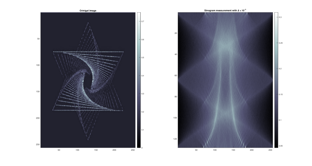
Figure 1: Data visualization:

Original image and its noisy sinogram measurement with $\delta=0.1\%$ from a rank deficient forward operator with dimensions $32768\times 65536$.

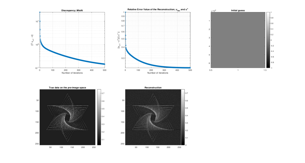
Figure 2: Error analysis profiles and data visualization with $\delta=0.1\%$ and matrix with the dimension of $32768\times 65536$:

Numerical results of the algorithm after it is applied on the underdetermined problem. In the reconstruction, we observe some artifacts as the traces of the lines that result from insufficient number of measurements. However, edges of the image are preserved due to TV penalization on the reconstruction. Relative error value of the final reconstruction falls below $0.3$.

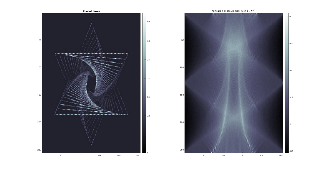
Figure 3: Data visualization:

Original image and its noisy sinogram measurement with $\delta=0.1\%$ from a full rank forward operator with the dimension of $65536\times 65536$.

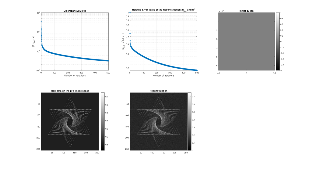
Figure 4: Error analysis profiles and data visualization with $\delta=0.1\%$ from a full-rank forward operator with dimensions $65536\times 65536$:

Unlike in the underdetermined system in Figure 2, relative error value of the final reconstruction falls below $0.2$. Also artifacts are less visible, and again edge preservation by TV penalization is observed.

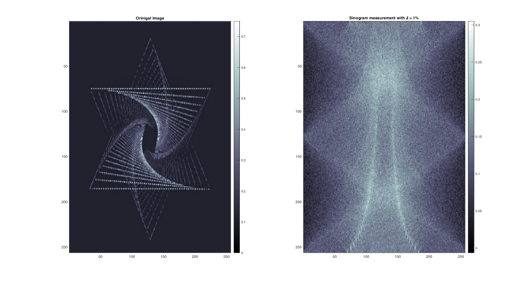
Figure 5: Data visualization:

Original image and its noisy sinogram measurement with $\delta=1\%$ from a full-rank matrix with dimensions $65536\times 65536$.

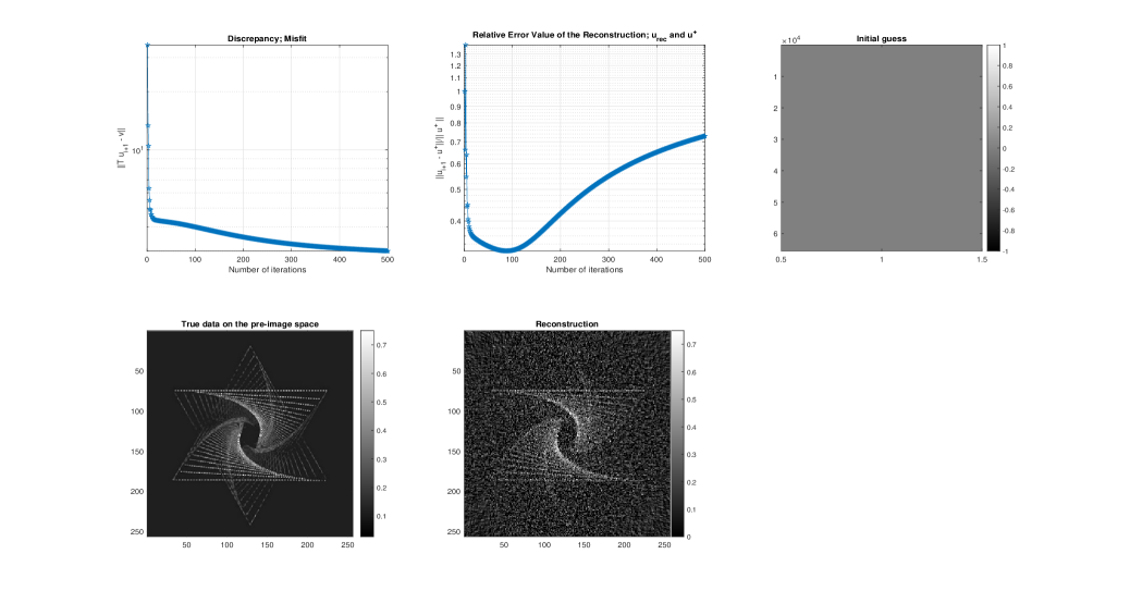
Figure 6: Error analysis profiles and data visualization:

Numerical results of the algorithm for a measurement with $\delta=1\%$ from a full-rank forward operator with dimensions of $65536\times 65536$. Since the noise level is high, the relative error estimation of the reconstructed data does not decay. That is consistent with the noise level observed in the reconstruction.

9 Discussion and Future Prospects

This work proposes some iterative regularization method evolved from some conventional optimization algorithm. We have observed that the choices of the parameters serve for the convergence analysis both in the Hadamard sense and in the iterative procedure sense. Furthermore, we must emphasize that the theoretical development for the stability analysis in the continous mathematical setting, i.e. the Hadamard convergence of the non-iterative regularized solution $u_{\alpha}^{\delta}$ to the minimum norm solution, is based on how the initial guess $u^{0}$ is chosen. We have been committed to make this selection due to mathematical difficulties appearing in the derivation of the Lemma 6.1, in particular on the inner products in the proof. However, it is our belief that with a different non-smooth analysis such difficulties can be overcome. Much of our theoretical results in the continuous setting are comparable with its counterparts available in the literature of variational regularization, see e.g. [39].

Regarding the stability analysis of the iterative approximation $u_{i},$ we have not needed to make any assumption on the initial guess $u_{0}.$ Instead, we have observed in Theorem 7.2 that initialization of the inner loop, i.e. the initial guess for the dual variable, is important for stating that $u_{i}$ is the approximation of $u_{\alpha}^{\delta}.$ Furthermore, the dynamical Bregman iterative form is maintained kby updating the dual variables.

Although we have used Morozov‘s discrepancy principle, further work could be done on the investigation of some Lepskij type stopping rule. Then a new convergence scheme is required for the iteratively regularized approximation $u_{i}$ towards the minimum norm solution.

In the numerical results, we have profiled the stability of the algorithm depending on the number of the measurements, see Figures 1 and 2. An open question still remains about the effect on recontruction of the angular arrangment of ray measurement.

Chapter APPENDIX

Appendix A VSC as Upper Bound for the Bregman Distance

The total error estimation can also be stabilized due to the following assumption that has been derived in the literature listed in Section 4.2,

$$E(u_{\alpha}^{\delta},u^{\dagger})\leq D_{\mathcal{J}}(u_{\alpha}^{\delta},u^{\dagger}).$$ (1.1)

Therefore, for stabilization of $E$, we seek a stable upper bound for the Bregman distance (1.1).

Assumption A.1.

[Variational Source Condition] Let $T:\mathcal{X}\rightarrow\mathcal{Y}$ be linear, injective forward operator and $v^{\dagger}\in\mathrm{range}(T).$ There exists some constant $\sigma\in(0,1]$ and a concave, monotonically increasing index function $\Psi$ with $\Psi(0)=0$ and $\Psi:[0,\infty)\rightarrow[0,\infty)$ such that for $q^{\dagger}\in\partial\mathcal{J}(u^{\dagger})$ the minimum norm solution $u^{\dagger}\in\mathrm{BV}(\Omega)$ satisfies

$$\sigma D_{\mathcal{J}}(u,u^{\dagger})\leq\mathcal{J}(u)-\mathcal{J}(u^{\dagger})+\Psi\left(\|Tu-Tu^{\dagger}\|\right)\mbox{, for all }u\in\mathcal{X}.$$ (1.2)

Recall that quantitative stability analysis in the continuous mathematical setting aims to find upper bound for the total error estimation functional $E$ in (4.4). According to (1.1), by means of finding stable upper bound for the Bregman distance between the regularized minimizer $u_{\alpha}^{\delta}$ and the minimum norm solution $u^{\dagger}$ will yield one of the two convergence results of this section. With the established choice of the regularization parameter and the asserted $\mathcal{J}$ difference estiamtion in Lemma 6.2, the last ingredient of the Bregman distance following up the Assumption A.1 is formulated below.

Lemma A.2.

Let $\alpha(\delta,v^{\delta})\in\overline{S}\cap\underline{S}$ be the regularization parameter for the regularized solution $u_{\alpha}^{\delta}$ to the problem (4.2). If the minimum norm solution $u^{\dagger}$ satisfies Assumption A.1, then

$$-\langle D^{\ast}w^{\dagger},u_{\alpha}^{\delta}-u^{\dagger}\rangle=\mathcal{O}(\Psi(\delta)),$$

holds.

Proof.

It follows from VSC (4.5) that

$$\frac{\sigma}{2}\left(\mathcal{J}(u_{\alpha}^{\delta})-\mathcal{J}(u^{\dagger})-\langle D^{\ast}w^{\dagger},u_{\alpha}^{\delta}-u^{\dagger}\rangle\right)\leq\mathcal{J}(u_{\alpha}^{\delta})-\mathcal{J}(u^{\dagger})+\Psi(\|Tu_{\alpha}^{\delta}-Tu^{\dagger}\|).$$ (1.3)

After arranging the terms,

$$-\langle D^{\ast}w^{\dagger},u_{\alpha}^{\delta}-u^{\dagger}\rangle \leq \frac{2}{\sigma}\left(1-\frac{\sigma}{2}\right)\left(\mathcal{J}(u_{\alpha}^{\delta})-\mathcal{J}(u^{\dagger})\right)+\Psi(\|Tu_{\alpha}^{\delta}-Tu^{\dagger}\|)$$ (1.4)

$$\stackrel{{\scriptstyle(\ref{J-diff2})}}{{\leq}} \frac{2}{\sigma}\left(1-\frac{\sigma}{2}\right)\left(\frac{1}{\underline{\tau}-1}\right)\Psi(\delta)+\Psi(\|Tu_{\alpha}^{\delta}-Tu^{\dagger}\|)$$

$$\stackrel{{\scriptstyle(\ref{consequence_MDP})}}{{\leq}} \frac{2}{\sigma}\left(1-\frac{\sigma}{2}\right)\left(\frac{1}{\underline{\tau}-1}\right)\Psi(\delta)+\Psi((\overline{\tau}+1)\delta)$$

$$\stackrel{{\scriptstyle(\ref{concave_id})}}{{\leq}} \frac{2}{\sigma}\left(1-\frac{\sigma}{2}\right)\left(\frac{1}{\underline{\tau}-1}\right)\Psi(\delta)+(\overline{\tau}+1)\Psi(\delta)$$

$$= \left(\frac{2}{\sigma}-1\right)\left(\frac{1}{\underline{\tau}-1}\right)\Psi(\delta)+(\overline{\tau}+1)\Psi(\delta).$$

∎

Theorem A.3.

Let the minimum norm solution $u^{\dagger}\in\Omega$ satisfy the VSC given by Assumption A.1. Then, in the light of the assumptions of lemmata 6.1, 6.2 and finally A.2, the following estimation holds,

$$D_{\mathcal{J}}(u_{\alpha}^{\delta},u^{\dagger})=\mathcal{O}(\Psi(\delta)).$$

Proof.

The proof simply follows from verifying the previously established estimations on each components of the Bregman distance as shown below,

$$D_{\mathcal{J}}(u_{\alpha}^{\delta},u^{\dagger}) = \mathcal{J}(u_{\alpha}^{\delta})-\mathcal{J}(u^{\dagger})-\langle D^{\ast}w^{\dagger},u_{\alpha}^{\delta}-u^{\dagger}\rangle$$ (1.5)

$$\stackrel{{\scriptstyle(\ref{VSC_innerprod})}}{{\leq}} \mathcal{J}(u_{\alpha}^{\delta})-\mathcal{J}(u^{\dagger})+\left(\frac{2}{\sigma}-1\right)\left(\frac{1}{\underline{\tau}-1}\right)\Psi(\delta)+(\overline{\tau}+1)\Psi(\delta)$$

$$\stackrel{{\scriptstyle(\ref{J-diff2})}}{{\leq}} \left(\frac{1}{\underline{\tau}-1}\right)\Psi(\delta)+\left(\frac{2}{\sigma}-1\right)\left(\frac{1}{\underline{\tau}-1}\right)\Psi(\delta)+(\overline{\tau}+1)\Psi(\delta).$$

∎

Appendix B Further Numerical Results

In this section, we will present some further numerical results to emphasize the condition on the step-length $\mu$ in Theorem 7.2. Although the formulated condition allows one to choose the step-length as $\mu=\frac{2}{\|T\|^{2}},$ we have observed divergence when we have made this choice of $\mu,$ see Figure 7.

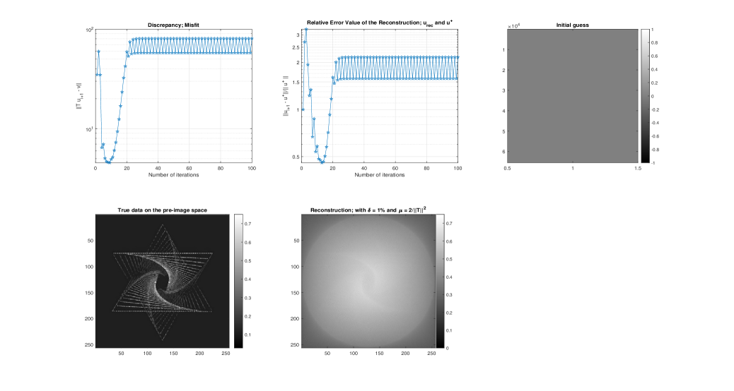
Figure 7: Error analysis profiles and the data visualization:

Although the noise amount is sufficiently small and it is a full rank system, with some different choice of the step-length that is defined as $\mu=\frac{2}{\|T\|^{2}},$ insufficient reconstruction and instability have been observed.

3 Acknowledgement

The author is indebted to Ignace Loris for the fruitful discussions throughout the development of the work. Furthermore, the author is highly grateful to Maria A. Gonzalez-Huici and David Mateos-Nunez for the encouragement and support to finalize the work. The work has been initiated by ARC grant at Université Libre de Bruxelles during author‘s PostDoc research period 2017 - 2019.

References

References

- [1] R. Acar, C. R. Vogel. Analysis of bounded variation penalty methods for ill-posed problems, Inverse Problems, Vol. 10, No. 6, 1217 - 1229, 1994.
- [2] E. Altuntac. Variational Regularization Strategy for Atmospheric Tomography. Institute for Numerical and Applied Mathematics, University of Goettingen, July 2016.
- [3] L. Ambrosio, N. Fusco, and D. Pallara. Functions of bounded variation and free discontinuity problems. Oxford Mathematical Monographs. The Clarendon Press, Oxford University Press, New York, 2000.
- [4] S. Anzengruber, B. Hofmann and P. Mathé. Regularization properties of the sequential discrepancy principle for Tikhonov regularization in Banach spaces. Appl. Anal. 93, 7, 1382 -1400, 2014.
- [5] S. Anzengruber and R. Ramlau. Morozov’s discrepancy principle for Tikhonov-type functionals with nonlinear operators. Inverse Problems, 26, 025001 (17pp), 2010.
- [6] S. Anzengruber and R. Ramlau. Convergence rates for Morozov’s discrepancy principle using variational inequalities. Inverse Problems, 27, 105007 (18pp), 2011.
- [7] M. Bachmayr and M. Burger. Iterative total variation schemes for nonlinear inverse problems, Inverse Problems, 25, 105004 (26pp), 2009.
- [8] H. H. Bauschke, P. L. Combettes. Convex analysis and monotone operator theory in Hilbert spaces, Springer New York, 2011.
- [9] J. M. Bardsley and A. Luttman. Total variation-penalized Poisson liklehood estimation for ill-posed problems, Adv. Comput. Math., 31:25-59, 2009.
- [10] A.Beck and M.Teboulle. A Fast Iterative Shrinkage-Thresholding Algorithm for Linear Inverse Problems. SIAM J. Imaging Sciences, Vol. 2, No. 1, pp. 183-202, 2009.
- [11] M. Benning and M. Burger. Modern Regularization Methods for Inverse Problems. https://arxiv.org/pdf/1801.09922, 2017.
- [12] M. Benning, M. M. Betcke, M. J. Ehrhardt, C.-B. Schönlieb. Choose your path wisely: gradient descent in a Bregman distance framework, arXiv:1712.04045, 2017.
- [13] M. Bergounioux. On Poincaré-Wirtinger inequalities in space of functions bounded variation. Control Cybernet., 40, 4, 921-29, 2011.
- [14] T. Bonesky, K. S. Kazimierski, P. Maass, F. Schöpfer, T. Schuster. Minimization of Tikhonov Functionals in Banach Spaces, Abstr. Appl. Anal., Art. ID 192679, 19 pp, 2008.
- [15] S. Bonettini, I. Loris, F. Porta, M. Prato and S. Rebegoldi. On the convergence of a linesearch based proimal-gradient method for nonconvex optimization. Inverse Problems, 33, 055005 (30pp), 2017.
- [16] J. Borwein and R. Luke. Entropic Regularization of the Function. In: Bauschke H., Burachik R., Combettes P., Elser V., Luke D., Wolkowicz H. (eds) Fixed-Point Algorithms for Inverse Problems in Science and Engineering. Springer Optimization and Its Applications, vol 49. Springer, New York, NY, 2011.
- [17] K. Bredies. A forward-backward splitting algorithm for the minimization of non-smooth convex functionals in Banach space, Inverse Problems 25, no. 1, 015005, 20 pp, 2009.
- [18] M. Burger, S. Osher. Convergence rates of convex variational regularization, Inverse Problems, 20(5), 1411 - 1421, 2004.
- [19] A. Chambolle. An algorithm for Total Variation Minimization and Applications. J. Math. Imaging Vis., 20, 89 - 97, 2004.
- [20] A. Chambolle, Vicent Caselles, Matteo Novaga, Daniel Cremers, Thomas Pock. An introduction to Total Variation for Image Analysis. hal-00437581, 2009.
- [21] A. Chambolle, P. L. Lions. Image recovery via total variation minimization and related problems, Numer. Math. 76, 167 - 188, 1997.
- [22] T. F. Chan and K. Chen. An optimization-based multilevel algorithm for total variation image denoising, Multiscale Model. Simul. 5, no. 2, 615-645, 2006.
- [23] T. Chan, G. Golub and P. Mulet. A nonlinear primal-dual method for total variation-baes image restoration, SIAM J. Sci. Comp 20: 1964-1977, 1999.
- [24] J. Chen and I. Loris On starting and stopping criteria for nested primal-dual iterations. arXiv:1806.07677, 2018.
- [25] F. H. Clarke. Optimization and Nonsmooth Analysis. Classics in Applied Mathematics, 5, SIAM, 1990.
- [26] D. Colton and R. Kress. Inverse Acoustic and Electromagnetic Scattering Theory, Springer Verlag Series in Applied Mathematics Vol. 93, Third Edition 2013.
- [27] P.L. Combettes and JC. Pesquet. Proximal Splitting Methods in Signal Processing. In: Bauschke H., Burachik R., Combettes P., Elser V., Luke D., Wolkowicz H. (eds) Fixed-Point Algorithms for Inverse Problems in Science and Engineering. Springer Optimization and Its Applications, vol 49. Springer, New York, NY, 2011.
- [28] M. Defrise, C. Vanhove, and X. Liu. An algorithm for total variation regularization in high-dimensional linear problems, Inverse Problems 27 065002 (16pp), 2011.
- [29] D. Dobson, O. Scherzer. Analysis of regularized total variation penalty methods for denoising, Inverse Problems, Vol. 12, No. 5, 601 - 617, 1996.
- [30] D. C. Dobson, C. R. Vogel. Convergence of an iterative method for total variation denoising, SIAM J. Numer. Anal., Vol. 34, No. 5, 1779 - 1791, 1997.
- [31] H. W. Engl, M. Hanke, A. Neubauer. Regularization of inverse problems, Math. Appl., 375. Kluwer Academic Publishers Group, Dordrecht, 1996.
- [32] J. Flemming. Existence of variational source conditions for nonlinear inverse problems in Banach spaces. J. Inverse Ill-Posed Probl., 26, 2, 277 - 286, 2018.
- [33] J. M. Fowkes, N. I. M. Gould, C. L. Farmer. A branch and bound algorithm for the global optimization of Hessian Lipschitz continuous functions, J. Glob. Optim., 56, 1792 - 1815, 2013.
- [34] G. Garrigos, L. Rosasco and S. Villa. Iterative regularization via dual diagonal descent. J Math Imaging Vis, 60, 2, 189 - 215, 2018.
- [35] M. Grasmair. Generalized Bregman distances and convergence rates for non-convex regularization methods, Inverse Problems 26, 11, 115014, 16pp, 2010.
- [36] M. Grasmair. Variational inequalities and higher order convergence rates for Tikhonov regularisation on Banach spaces, J. Inverse Ill-Posed Probl., 21, 379-394, 2013.
- [37] M. Grasmair, M. Haltmeier, O. Scherzer. Necessary and sufficient conditions for linear convergence of -regularization, Comm. Pure Appl. Math. 64(2), 161-182, 2011.
- [38] B. Hofmann, B. Kaltenbacher, C. P‘̀oschl, and O. Scherzer. A convergence rates result for Tikhonov regularization in Banach spaces with non-smooth operator. Inverse Problems, 23 (3), 987 - 1010, 2007.
- [39] B. Hofmann and P. Mathé. Parameter choice in Banach space regularization under variational inequalities. Inverse Problems 28, 104006 (17pp), 2012.
- [40] T. Hohage and F. Weidling. Verification of a variational source condition for acoustic inverse medium scattering problems. Inverse Problems, 31, 075006 (14pp), 2015.
- [41] T. Hohage and C. Schormann. A Newton-type method for a transmission problem in inverse scattering. Inverse Problems 14, 1207 - 1227, 1998.
- [42] T. Hohage and F. Weidling. Characterizations of variational source conditions, converse results, and maxisets of spectral regularization methods. arXiv:1603.05133, 2016.
- [43] V. Isakov. Inverse problems for partial differential equations. Second edition. Applied Mathematical Sciences, 127. Springer, New York, 2006.
- [44] S. Kindermann. Convex Tikhonov regularization in Banach spaces: New results on convergence rates. J. Inverse Ill-Posed Probl., 24, 3, 341 - 350, 2016.
- [45] A. Kirsch. An introduction to the mathematical theory of inverse problems. Second edition. Applied Mathematical Sciences, 120. Springer, New York, 2011.
- [46] D. A. Lorenz. Convergence rates and source conditions for Tikhonov regularization with sparsity constraints, J. Inv. Ill-Posed Problems, 16, 463-478, 2008.
- [47] I. Loris and C. Verhoeven. On a generalization of the iterative soft-thresholding algorithm for the case of non-separable penalty. Inverse Problems, 27, 125007, 15pp, 2011.
- [48] C. Louchet and L. Moisan. Total Variation as a Local Filter. SIAM J. IMAGING SCIENCES, Vol. 4, No. 2, pp. 651 - 694, 2011.
- [49] S. Osher, M. Burger, D. Goldfarb, J. Xu and W. Yin. An Iiterative Regularization Method for Total Variation-Based Image Restoration. Multiscale Model. Simul., 4(2), 460 - 489, 2005.
- [50] R.T. Rockafellar, R. J.-B. Wets. Variational Analysis. Fundamental Principles of Mathematical Sciences, 317. Springer-Verlag, Berlin, 1998.
- [51] L. I. Rudin, S. J. Osher, E. Fatemi. Nonlinear total variation based noise removal algorithms, Physica D, 60, 259-268, 1992.
- [52] O. Scherzer, M. Grasmair, H. Grossauer, M. Haltmeier and F. Lenzen. Variational Methods in Imaging. Applied Mathematical Sciences, 167, Springer, New York, 2009.
- [53] T. Schuster, B. Kaltenbacher, B. Hofmann, K.S. Kazimierski. Regularization Methods in Banach Spaces. RICAM, 10, De Gruyter, 2012.
- [54] D. F. Shanno and K. Phua. Matrix conditioning and nonlinear optimization. Math. Prog., 14, 149 - 160, 1978.
- [55] B. Sprung and T. Hohage. Higher order convergence rates for Bregman iterated variational regularization of inverse problems. arXiv:1710.09244, 2017.
- [56] W. Takahashi, N.C. Wong and J.C. Yao. Fixed point theorems for nonlinear non-self mappings in Hilbert spaces and applications. JFPTA, 2013:116, 2013.
- [57] A. N. Tikhonov. On the solution of ill-posed problems and the method of regularization, Dokl. Akad. Nauk SSSR, 151, 501-504, 1963.
- [58] A. N. Tikhonov, V. Y. Arsenin. Solutions of ill-posed problems. Translated from the Russian. Preface by translation editor Fritz John. Scripta Series in Mathematics. V. H. Winston & Sons, Washington, D.C.: John Wiley & Sons, New York-Toronto, Ont.-London, xiii+258 pp, 1977.
- [59] C. R. Vogel. Computational methods for inverse problems, Frontiers Appl. Math. 23, 2002.
- [60] C. R. Vogel , M. E. Oman. Iterative methods for total variation denoising, SIAM J. SCI. COMPUT., Vol. 17, No. 1, 227-238, 1996.
- [61] W. Yin, S. Osher, D. Goldfarb and J. Darbon. Bregman Iterative Algorithms for Minimization with Applications to Compressed Sensing. SIAM J. Imaging Sciences, Vol. 1, N0. 1, pp.143 - 168, 2008.
- [62] Zeidler E. Applied functional analysis application to mathematical physics. Applied Mathematical Sciences, 108. Springer-Verlag, New York, 1995.