Structure, dynamics and reconnection of vortices in a non-local model of superfluids

Abstract

We study the reconnection of vortices in a quantum fluid with a roton minimum, by numerically solving the Gross-Pitaevskii (GP) equations. A non-local interaction potential is introduced to mimic the experimental dispersion relation of superfluid ${}^{4}\mathrm{He}$. We begin by choosing a functional shape of the interaction potential that allows to reproduce in an approximative way the so-called roton minimum observed in experiments, without leading to spurious local crystallization events. We then follow and track the phenomenon of reconnection starting from a set of two perpendicular vortices. A precise and quantitative study of various quantities characterizing the evolution of this phenomenon is proposed: this includes the evolution of statistics of several hydrodynamical quantities of interest, and the geometrical description of a observed helical wave packet that propagates along the vortex cores. Those geometrical properties are systematically compared to the predictions of the Local Induction Approximation (LIA), showing similarities and differences. The introduction of the roton minimum in the model does not change the macroscopic properties of the reconnection event but the microscopic structure of the vortices differs. Structures are generated at the roton scale and helical waves are evidenced along the vortices. However, contrary to what is expected in classical viscous or inviscid incompressible flows, the numerical simulations do not evidence the generation of structures at smaller or larger scales than the typical atomic size.

I Introduction

Turbulence in quantum fluids is the study of the motions induced by a tangle of quantum vortices, which are created under a large-scale stirring force, or in the presence of a counter-flow generated by a hot source (see for instance the reviews Vinen and Niemela (2002); Tsubota (2008); Paoletti and Lathrop (2011); Barenghi et al. (2014a, b)). In practice, it can be investigated in a variety of physical systems, e.g. in cold atoms Bose-Einstein condensates Horng et al. (2008); Cidrim et al. (2017), superfluid ${}^{3}\mathrm{He}$ Blaauwgeers et al. (2002); Bradley et al. (2008), or superfluid ${}^{4}\mathrm{He}$ Maurer and Tabeling (1998); Zhang and Sciver (2005). In this paper, we focus on the case of superfluid ${}^{4}\mathrm{He}$, which is obtained when liquid ${}^{4}\mathrm{He}$ is cooled at temperatures below $T_{\lambda}\approx$2.17\text{\,}\mathrm{K}$$ (at saturated vapor pressure). At finite temperature, the fluid is made up of a mixture of two components, one being classical and viscous, governed by the incompressible Navier-Stokes equation, and the other one being inviscid, compressible and potential with localized and quantized singularities (i.e. quantum vortices) hosting the rotational motions. These two components interact in a subtle way through the friction of these vortices onto the viscous component, a phenomenon that allows the decay of fluctuations of the quantum component without thus the action of viscosity. Macroscopically, i.e. at scales larger than the dissipative scale of the classical component, statistics of velocity fluctuations in this mixture look very similar to the ones observed in classical three-dimensional turbulence, as depicted in the phenomenology of Kolmogorov Frisch (1995). This includes the fine scale structure of turbulence, such as the power-law decrease of the velocity spectrum and higher-order (i.e. intermittent) properties Maurer and Tabeling (1998); Abid et al. (1998); Salort et al. (2010); Varga et al. (2018), scale-energy transfers (i.e. the skewness phenomenon) Salort et al. (2012), and also the global behavior at large scales Saint-Michel et al. (2014). Even if some differences have been highlighted between quantum and classical turbulence Paoletti et al. (2008); White et al. (2010) at the level of an isolated quantum vortex, it is thus tempting to consider that at a finite temperature below $T_{\lambda}$, the two components are locked at each others, implying that quantum vortices self-organize, forming structures (i.e. bundles) such that the overall locally averaged vorticity field of the superfluid component resembles to the one observed in classical turbulence Vinen and Niemela (2002); Tsubota (2008); Paoletti and Lathrop (2011); Barenghi et al. (2014a, b). At smaller scales, typically below the mean inter-vortex distance, a decoupling of the two components is nonetheless expected Salort et al. (2011), superfluid velocity fluctuations being governed by other phenomena such as Kelvin waves propagation along vortex cores Kozik and Svistunov (2004); L’vov et al. (2007).

Such scales are difficult to access experimentally, thus from a modeling point of view, it is tempting to study the collective effects of a population of localized singularities hosting a distributional repartition of vorticity, in particular in interaction with an exterior (classical) velocity field. A popular method to study the interaction between these vortices is given by the Vortex Filament (VF) model, where the velocity field induced by a vortex is described by the Biot-Savart law. In the case where the vortex core size is negligible compared to its local curvature, it is interesting to consider the Local Induction Approximation (LIA) Schwarz (1985, 1988) of the VF model, that takes only into account the induced velocity field of a local portion of the vortex. Such an approach can then be generalized to take into account non local effects induced by the whole vortex Adachi et al. (2010); Baggaley (2012), in order to study the dynamics of an ensemble of vortices and the implication of non local effects. In this context, a phenomenon of tremendous importance is vortex reconnection, that allows for dissipation and a possible change in the macroscopic distribution of these vortices, that has to be put by hand at this stage.

An alternative approach devoted to the dynamics of vortices and their interaction, that might be of some interest in the improvements of the aforementioned discrete approaches, neglecting the coupling with a normal component and assuming vanishing temperature $T=0$, is given by the description and evolution of the order parameter of the superfluid in terms of fields, as it is proposed by a partial differential equation known as the Gross-Pitaevskii (GP) equation Pitaevskii and Stringari (2003). Contrary to the approach based on the LIA, the GP equation naturally includes vortex reconnection, without thus asking for further modeling steps. This approach has been studied extensively in the literature Koplik and Levine (1993); Nore et al. (1997). In this approach, that allows to study some global behavior of an assembly of vortices at scales of the order of the inter-vortex distance, their very internal structure is neglected and the two body interaction usually adopted is of localized (i.e. distributional) type. The purpose of this article is the numerical study of a non-local version of the GP equations that allows to reproduce a realistic internal structure of these vortices and observe and quantify its implication on vortex reconnection, and on possible wave packet propagation along their cores. This can be done while introducing in the interaction potential a physical length scale $a$ representing the typical size of a ${}^{4}\mathrm{He}$ atom.

II A non local model of superfluids including the roton minimum, and its calibration

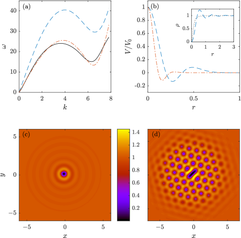
Figure 1: (a): Dispersion relations of ${}^{4}\mathrm{He}$ and its model as given by the non-local GP equation (Eq. 1): experimental results from neutron scattering experiments (black line, see Ref. Donnelly and Barenghi (1998)), its fit as proposed in Ref. Berloff and Roberts (1999) (red dashed-dotted line), and our current model (Eq. 3) with a raised roton minimum so as to avoid crystallization as explained in the text (blue dashed line). (b): Corresponding interaction potentials $V(r)/V_{0}$ entering in Eq. 1, with $V_{0}=21.96\,\mbox{eV}$ for the model of Ref. Berloff and Roberts (1999) $V_{0}=0.15\,\mbox{eV}$ for our present model (Eq. 3), used to obtain the theoretical dispersion curves of (a). We display in the inset the radial density profile of the stationary solution corresponding to the local GP equation (Eq. 10) with a black dotted line, and the corresponding profile in the non-local case (Eq. 1) with a blue dashed line. (c) and (d): Color plots of the distribution of density, i.e. $|\psi|^{2}$, of the stationary vortex solution obtained as the solution of the relaxation problem given in Eq. 4. (c): with our raised roton gap (Eq. 3) so as to avoid crystallization. (d): with the potential proposed in Ref. Berloff and Roberts (1999), which leads to a crystallization event.

At zero temperature $T=0$, to the lowest approximation we can consider the superfluid under study to be described by a scalar wave function $\psi$, i.e. an order parameter, which is space and time dependent. Henceforth, we consider dimensionless coordinates ${\mbox{\boldmath$r$}}\in\mathbb{R}^{3}$ and $t\in\mathbb{R}$ by respectively the roton wavelength $a=$3.26\text{\,}\mathrm{\SIUnitSymbolAngstrom}$$ Pitaevskii and Stringari (2003); Donnelly and Barenghi (1998) and a quantum typical time $t_{0}=2ma^{2}/\hbar=$1.34\text{\times}{10}^{-11}\text{\,}\mathrm{s}$$, where $m=$6.65\text{\times}{10}^{-27}\text{\,}\mathrm{k}\mathrm{g}$$ corresponds to the ${}^{4}\mathrm{He}$ atom mass. Considering that the number of atoms is high in the condensate, we can assume that the dynamics of $\psi$ is given by the GP equation, that reads in its most general and dimensionless version

$$i\frac{\partial\psi}{\partial t}=-\Delta\psi+(V\ast|\psi|^{2})\psi-\mu\psi,$$ (1)

where $V({\mbox{\boldmath$x$}})$ is a smooth two-body interaction potential, assumed to be spherically symmetrical (a function of the norm $x=|{\mbox{\boldmath$x$}}|$ only), $\ast$ stands for the convolution product, i.e. $(V\ast|\psi|^{2})({\mbox{\boldmath$x$}},t)=\int V({\mbox{\boldmath$x$}}-{\mbox{\boldmath$y$}})|\psi|^{2}({\mbox{\boldmath$y$}},t)\,d^{3}y$, and $\mu=\int V({\mbox{\boldmath$x$}})\,d^{3}x$ the chemical potential ensuring $|\psi|^{2}=1$ as a homogeneous solution. As it is shown in Refs. Pomeau and Rica (1993); Berloff and Roberts (1999); Villerot et al. (2012), the finite extension of the interaction potential is crucial in obtaining a dispersion relation that reproduces the roton minimum, as it is observed in neutron scattering measurements performed in superfluid ${}^{4}\mathrm{He}$ Donnelly and Barenghi (1998); Fåk et al. (2012). This allows us to calibrate the superfluid model that is proposed in Eq. 1 while computing the dispersion relation, readily obtained as

$$\omega^{2}({\mbox{\boldmath$k$}})=|{\mbox{\boldmath$k$}}|^{4}+2|{\mbox{\boldmath$k$}}|^{2}\widehat{V}({\mbox{\boldmath$k$}}),$$ (2)

where $\widehat{V}({\mbox{\boldmath$k$}})=\int e^{i{\mbox{\boldmath$k$}}.{\mbox{\boldmath$x$}}}V({\mbox{\boldmath$x$}})d^{3}x$ is the Fourier transform of the interaction potential, which depends only on $k=|{\mbox{\boldmath$k$}}|$ if $V$ is taken isotropic. To get the dispersion relation (Eq. 2), we use standard techniques consisting in linearizing Eq. 1 while looking for solution of the form $\psi=1+\varphi$, for small $\varphi$, Fourier transforming the linear dynamics of $\varphi$ and its conjugate, then looking for constraints on $\omega$ and $|{\mbox{\boldmath$k$}}|$ to avoid a single trivial solution (see Pomeau and Rica (1993); Berloff and Roberts (1999); Villerot et al. (2012)). Choosing a particular form for $\widehat{V}({\mbox{\boldmath$k$}})$ allows then to compare the so-obtained dispersion relation against experimental measurements.

In subsequent numerical simulations that we will present in the next sections, we choose the following functional isotropic form for the interaction potential

$$\widehat{V}({\mbox{\boldmath$k$}})=\left(\frac{c_{s}^{2}}{2}-v_{1}^{2}|{\mbox{\boldmath$k$}}|^{2}+v_{2}^{4}|{\mbox{\boldmath$k$}}|^{4}\right)\exp\left(-\frac{\left|{\mbox{\boldmath$k$}}\right|^{2}}{2k_{0}^{2}}\right),$$ (3)

where $c_{s}$ corresponds to the sound velocity, i.e. the limit at small wave-vector of $\omega^{2}({\mbox{\boldmath$k$}})/|{\mbox{\boldmath$k$}}|$, and $(v_{1},v_{2},k_{0})$ three free parameters than could be obtained for example using a least-square fit procedure given a experimental dispersion relation. We will not do that and use instead, within our choice of units, $c_{s}=16$, $v_{1}=2.2635$, $v_{2}=0.4408$ and $k_{0}=5.5970$. We now motivate our choice and compare against experimental data.

We represent in Fig. 1 (a) the dispersion relation of liquid ${}^{4}\mathrm{He}$ at saturated vapor pressure provided in Ref. Donnelly and Barenghi (1998) using a solid black line, and that exhibits indeed a roton minimum around $|{\mbox{\boldmath$k$}}|=2\pi$. We superimpose there using a red dashed-dotted line the dispersion relation obtained with the model proposed in Ref. Berloff and Roberts (1999), which implications on the vortex density profile are discussed in section V. With a blue dashed line, we represent the dispersion relation we get, using Eq. 2, with an interaction potential (Fourier transformed) given in Eq. 3 that we use in subsequent numerical simulations, with the formerly defined free parameters $(v_{1},v_{2},k_{0})$ and the given sound velocity $c_{s}$. The corresponding potential profiles in real space are represented in Fig. 1 (b). We observe quantitative differences between the experimental and our theoretical dispersion relations. First, when expressed in physical units, we have chosen a sound velocity of the order of $354\text{\,}\mathrm{m}\mathrm{/}\mathrm{s}$, which is higher than the observed value $238\text{\,}\mathrm{m}\mathrm{/}\mathrm{s}$. This explains why experimental and theoretical curves deviate at vanishing $|{\mbox{\boldmath$k$}}|$. Furthermore, we see that the theoretical curve reproduces the correct value of the roton wavevector $|{\mbox{\boldmath$k$}}|=2\pi$, but not the value of the of the minimum of angular frequency $\omega$ (nor consistently the value of the maxon, i.e. the local maximum of frequency occurring just before). This choice is dictated by further numerical investigations in which we forbid any crystallization phenomena, a natural tendency of this type of model (Eq. 1) to evolve toward a periodical modulations of density $\rho=|\psi|^{2}$, as it has been exploited to describe a possible supersolid-state of matter Pomeau and Rica (1994); Josserand et al. (2007). This tendency to crystallization is described in section IV. At this stage, let us state that the present approach, based on a scalar wave function with a two-body non-local interaction as considered in Eq. 1 is unable to describe the dynamics of ${}^{4}\mathrm{He}$ in a superfluid phase with a more realistic dispersion relation.

Indeed, let us show that such a choice for the interaction potential (Eq. 3) allows axisymmetric stationary solutions, i.e. vortex-lines with quantized circulation, as it has been widely studied for the local GP equation Pitaevskii and Stringari (2003).

III A detour through the numerical estimation of axisymmetric stationary solutions

A major success of scalar wave functional approaches, and its related dynamics given by the GP equation Pitaevskii and Stringari (2003), lies in the existence of a stationary solution (i.e. time independent) which is axisymmetric (say independent of the $z$ coordinate and on the polar angle $\varphi$ in the $xy$-plane) and exhibiting a $2\pi$ defect for the phase. More precisely, a solution of the form $\psi(r,\varphi,z)=\sqrt{\rho(r)}e^{i\varphi}$, where we have introduced the polar decomposition of the wave function in terms of amplitude and phase, and the cylindrical coordinates $(r,\varphi,z)$ in which $x=r\cos(\varphi)$ and $y=r\sin(\varphi)$. To numerically estimate the shape of the density distribution $\rho(r)$ as a function of the polar distance $r$, and more generally to test the existence of such a axisymmetric solution, we numerically solve the two-dimensional relaxation problem (corresponding to the propagation of Eq. 1 in imaginary time with the $z$-independence as a constraint)

$$\frac{\partial\psi}{\partial t}=\left(\frac{\partial^{2}}{\partial x^{2}}+\frac{\partial^{2}}{\partial y^{2}}\right)\psi-(\widetilde{V}\ast|\psi|^{2})\psi+\mu\psi,$$ (4)

with initial condition $\psi(x,y,0)=e^{i\varphi(x,y)}$, $\varphi(x,y)=\arctan(y/x)$ (the inverse tangent being suitably defined), and $\widetilde{V}(x,y)=\int V(x,y,z)\,dz$. We solve this initial value problem using periodic boundary conditions in order to efficiently compute linear operations in the Fourier space, and nonlinear ones in the physical space. Doing so, in order to prevent from phase discontinuities, we use four copies of this initial condition with appropriate phase distribution, and evenly spaced, as it is explained and performed in Ref. Koplik and Levine (1993). In units of the length scale $a$, we use as a mesh size $dx=1/16$, and depending on the number of collocation points $N$ in each direction, we consider domains of physical size $Ndx$. Using thus $N=512$ (vortices are sufficiently far apart to neglect their interaction), we simulate a domain of physical size $32\,a\approx 100\mathrm{\AA}$. Time propagation is performed using a fourth-order Runge-Kutta explicit method with $dt={(dx)}^{2}/64$, corresponding to $8.2\text{\times}{10}^{-16}\text{\,}\mathrm{s}$ in physical units. This particular value for the time-step was obtained by starting from the numerical stability prediction for the heat equation $dt\leq dx^{2}/2$ Press et al. (2007), and then decreasing $dt$ until all simulations were numerically stable. To prevent from spurious generation of unphysical small scales, we use as a dealiasing method the $2/3$-rule, each time we perform a multiplication in the physical space. In our case, since the nonlinearity is of order three, we apply this rule two times at each time step, which is enough to prevent the generation of unphysical small scales.

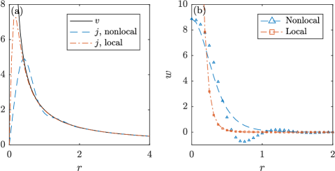
Figure 2: (a) Radial distributions of the velocity field $v$ and probability current $j$ of the axisymmetric stationary solutions of the local (Eq. 10) and non-local (Eq. 1) GP equations. (b) Radial distributions of the associated pseudo-vorticity fields (Eq. 8), and their comparison with a schematic fit provided in Eq. 9.

Starting from our initial condition, we observe the convergence of Eq. 4 toward a time-independent solution that we can consider as a stationary solution of the non-local GP equation (Eq. 1) itself, and we represent it in Fig. 1 (c). We see that indeed the solution is symmetrical around the axis of the vortex, where the density tends to zero, as it is expected at the core of quantum vortices. We furthermore see the existence of additional density oscillations around the vortex core, which are themselves expected once a roton minimum is included in the picture. This is a well-known phenomenon Regge (1972); Dalfovo (1992); Berloff and Roberts (1999); Rossi et al. (2012); Villerot et al. (2012); Molinelli et al. (2016), for which density oscillations are prescribed by the characteristic shape and size of the roton minimum. We represent in the inset of Fig. 1 (b) a comparison of the density profile away from the vortex core obtained in axisymmetric stationary solutions of the local (given in Eq. 10, curve is in black) and non-local GP equations (our present numerical estimation) where we see more clearly that the presence of the roton minimum leads to periodical modulation of density, governed by the roton characteristics, and can be seen as precursors of the crystallization phenomenon Pomeau and Rica (1994); Josserand et al. (2007).

IV Further comments on the model of the interaction potential

We represent (red dashed-dotted line) in Fig. 1 (a) the model of the non-local interaction potential $V$ chosen in Ref. Berloff and Roberts (1999), which also includes an additional quintic term in the overall dynamics. It does reproduce with great accuracy the experimental dispersion relation of Ref. Donnelly and Barenghi (1998). Nonetheless, when looking for a possible axisymmetric stationary solution, in the spirit of the relaxation problem posed in Eq. 4, we end up eventually with a time-independent solution displayed in Fig. 1 (d). We see that in this case, the invariance around the axis of the vortex is broken by the appearance of additional periodic modulation of density that form a hexagonal structure. This crystallization phenomenon was already observed in early numerical simulations of the non-local GP equation Berloff (1999), where it is associated to a phenomenon of mass concentration associated to negative values of the interaction potential. Remark also that we could have used also another set of parameters $(c_{s},v_{1},v_{2},k_{0})$ in order to be much closer to the experimental dispersion curve, and without including an additional quintic term. Similarly to the model proposed in Ref. Berloff and Roberts (1999), the corresponding stationary vortex solution would also exhibit such a crystallization phenomenon (data not shown). We performed similar simulations using domains of larger sizes (up to $2048^{2}$ collocation points using the same $dx$, and not displayed here for the sake of clarity) and observe a similar crystallization phenomenon with the same period. As we will comment while evoking the notion of supersolidity as it is discussed in Refs. Pomeau and Rica (1994); Josserand et al. (2007), the period of such a precursor of crystallization is governed by the finite extension of the interaction potential, and is thus not influenced by the macroscopic scale of the domain. Let us furthermore mention that these stationary solutions are obtained while solving a 2D relaxation problem, which includes as an additional constraint the translational invariance along the vortex axis (Eq. 4 is readily obtained from Eq. 1 assuming independence on the spatial variable $z$). Thus, these density oscillations should be furthermore seen as being independent of the $z$-direction, which is physically barely acceptable. For these reasons, we decide to look for a set of parameters $(c_{s},v_{1},v_{2},k_{0})$ that would allow a non-crystallized stationary vortex solution.

In the light of more recent studies Pomeau and Rica (1994); Josserand et al. (2007) concerning the natural evolution toward the state of supersolidity when a roton minimum is included in the picture, we are left with concluding that a GP type of evolution, where enters a simple non-local two-body interaction (with a possible additional quintic term), is unable to describe in a proper manner superfluid ${}^{4}\mathrm{He}$ if we follow with great accuracy the experimental dispersion curve of Ref. Donnelly and Barenghi (1998). Let us note that, to our knowledge, there is no experimental evidence of the very microscopic structure of vortices in superfluid helium at the roton scale. As a consequence, we cannot affirm that such a crystalline structure is impossible in ${}^{4}\mathrm{He}$. However, at a macroscopic scale, non-crystallized vortices are well supported by experimental evidence in superfluid Helium Yarmchuk et al. (1979) and in atomic Bose Einstein Condensates (BEC) Wilson et al. (2015). In other words, we ask the model of superfluid we consider and given in Eq. 1 to exhibit a non-crystallized vortex (i.e. axisymmetric) as a possible stationary solution. To do so, we are led to use an interaction potential $V$ which is unable to reproduce with great accuracy the experimental dispersion curve. Note nonetheless that calibrating our model, which involves a nonlinearity in the evolution (Eq. 1), using the dispersion relation, that is a prediction obtained through a linearization procedure, is difficult to control. It would be of great interest to develop a new type of dynamics that would include both a correct description of the experimental dispersion relation, and the existence of stationary axisymmetric solutions representing in a proper way quantum vortices. We leave this aspect for future investigations, and perform subsequent three dimensional numerical simulations with the aforementioned model for the interaction potential (Eq. 2), that prevents the formation of these hexagonal periodic modulations of density.

V Spatial distribution of the vortex solution

Let us now investigate the very radial distribution of various kinematic quantities entering in the hydrodynamical interpretation of the non-local GP equation (Eq. 1), as it is given by the Madelung transformation Pitaevskii and Stringari (2003). In this approach, we associate the gradient of the phase of $\psi$ to a velocity field v and $|\psi|^{2}$ to a local density field $\rho$. Key kinematic quantities are thus density $\rho=|\psi|^{2}$ and probability current ${\mbox{\boldmath$j$}}=-i(\psi^{*}{\mbox{\boldmath$\nabla$}}\psi-\psi{\mbox{\boldmath$\nabla$}}\psi^{*})=\rho{\mbox{\boldmath$v$}}$ that are governed by conservation equations that read Berloff and Roberts (1999); Nore et al. (1997); Pitaevskii and Stringari (2003)

$$\frac{\partial\rho}{\partial t}+{\mbox{\boldmath$\nabla$}}.{\mbox{\boldmath$j$}}=0,$$ (5)

that can be interpreted as a continuity equation, and considering a component $j_{i}$ of the vector $j$, we have

$$\frac{\partial j_{i}}{\partial t}+\partial_{j}\Pi_{ij}=0,$$ (6)

where $\Pi_{ij}$ is the momentum tensor,

$$\Pi_{ij}=\partial_{i}\psi\partial_{j}\psi^{*}-\psi\partial^{2}_{ij}\psi^{*}+\mbox{c.c.}+\frac{1}{2}\rho(V\ast\rho)\delta_{ij},$$ (7)

where c.c. stands for the complex conjugate, and $\delta_{ij}$ the Kronecker symbol. Similarly, we could derive the time evolution of the velocity field $v$, which corresponds to a compressible, irrotational and barotropic fluid with an additional quantum pressure term, of density corresponding to $|\psi|^{2}$ (see for instance Refs. Berloff and Roberts (1999); Berloff (1999)). It is well known that the velocity field diverges in the vicinity of a defect of the phase, so we will in the next sections work with the current vector $j$, that is eventually, as we are going to see, a bounded vector.

We display in Fig. 2 (a) the radial profile of velocity $v$ and probability current $j$ of the axisymmetric stationary solution represented in Fig. 1 (d). Let us recall that, using cylindrical coordinates centered on the vortex, the velocity field ${\mbox{\boldmath$v$}}=1/r\,{\mbox{\boldmath$e$}}_{\theta}$ and the current ${\mbox{\boldmath$j$}}=\rho(r)/r\,{\mbox{\boldmath$e$}}_{\theta}$ are known. Remark that $|{\mbox{\boldmath$v$}}|=1/r$, as we mentioned, diverges in the vicinity of the vortex line, whereas $j$ is a bounded vector since $\rho(r)$ tends to 0 as $r^{2}$ Pitaevskii and Stringari (2003) in the vicinity of the origin (so that $j$ vanishes itself at the origin). This is what is indeed obtained and displayed in Fig. 2 (a). We furthermore superimpose the radial distribution of $j$ that is obtained from the local, i.e. standard, version of the GP equation, that we define precisely later (see Eq. 10). Once again, we see that the current follows a non monotonic radial behavior. Compared to what is obtained in the non-local GP equation (Eq. 1), we can see that the maximum of current is obtained at a similar distance from the axis of symmetry in both models, but its value is higher in the non-local version of the dynamics.

Of great interest also from a dynamical point of view is the radial distribution of the pseudo-vorticity

$${\mbox{\boldmath$w$}}={\mbox{\boldmath$\nabla$}}\wedge{\mbox{\boldmath$j$}},$$ (8)

which quantifies the rotational motions of this compressible fluid. In the following, we note $w=\left|{\mbox{\boldmath$w$}}\right|$ the amplitude of pseudo-vorticity. For a single vortex line along the $z$ axis, $w$ is aligned with ${\mbox{\boldmath$e$}}_{z}$, and its amplitude only depends on the radial distance $r$ to the axis, and we have $w(r)=(1/r)d\rho(r)/dr$. Recall that vorticity itself, i.e. the curl of the velocity field $v$, is of distributional nature, and vanishes everywhere except at the very center of the vortex core where it diverges. Instead, as we can see in Fig. 2 (b), $w$ as defined in Eq. 8, is a bounded quantity.

In the local case (red symbols), we can even see that the radial distribution of pseudo-vorticity, as far as the axisymmetric solution is concerned, follows a monotonic decrease away from its axis of symmetry. As we see in section VI, in particular to interpreted some quantities entering in a statistical description of the flow, it is interesting to design a model for this radial behavior. For this purpose, we propose the following decreasing function

$$w(r)=\frac{w_{0}}{{\left[1+{\left(\frac{r}{r_{0}}\right)}^{2}\right]}^{\alpha}},$$ (9)

where $w_{0}$ is the value of pseudo-vorticity on the axis of symmetry, and $(r_{0},\alpha)$ two free parameters describing the shape of pseudo-vorticity radial distribution. Starting with the radial distribution of $w$ obtained from the local GP equation (and presented later in Eq. 10), the fit (Eq. 9) reproduces in a fairly good way the observed decrease using $r_{0}=0.22$ (in units of $a$) and $\alpha=3.125$. In a non-local context setting, as given by Eq. 1, such a fit reproduces accurately the decrease with $r_{0}=0.62$ and same $\alpha$, but obviously fails at reproducing the non monotonic behaviors associated to the additional oscillations associated to the roton minimum. As we will see in section VI, even if some aspects are not reproduced by such a schematic fit (Eq. 9), it will be very useful to interpret subsequent statistical quantities that we will observe in the next sections.

Let us also remark that the exponent $\alpha\approx 3.125$ is not that close to the value $2$, a typical value that is expected while considering the boundary value problem related to the spatial distribution of vortex density. Indeed, far from the vortex origin, and neglecting second order variations, density should reach the uniform solution as the square of the inverse of the distance from the vortex Pitaevskii and Stringari (2003). Using then $w(r)=(1/r)d\rho(r)/dr$, we easy get that pseudo-vorticity amplitude should tend to zero as $1/r^{4}$, corresponding thus to $\alpha=2$. In our case, we are looking at the behavior of pseudo-vorticity over a range that cannot be considered as being far from the origin of the vortex, namely over say one atomic distance (see the obtained values for the parameter $r_{0}$). Moreover, our simulation domain is finite, and copies, that are necessary to prevent from phase discontinuities in this periodical set-up, might interact in a subtle way such that the value $\alpha\approx 3.125$ reproduces in a better way the decrease of the pseudo-vorticity that we are observing. This may explain why we are not observing a $1/r^{4}$-decrease of pseudo-vorticity.

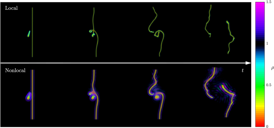
Figure 3: 3D visualization of the superfluid density during reconnection, in the local (top) and non-local (bottom) models. A density threshold is applied for clarity, so that the bulk fluid density $\rho\sim 1$ is transparent. Four snapshots are represented along time, from left to right respectively: the initial condition $t=0$, the reconnection time $t=t_{\text{rec}}$, twice the reconnection time $t=2t_{rec}$, and the end time of the simulation $t=t_{\text{end}}\approx 6t_{0}$.

VI Numerical investigation of reconnection of a set of initially perpendicular vortices

Let us now investigate the dynamics of vortex reconnection in the presence of a roton minimum, and thus with a non-local interaction potential (Eq. 1), as it was studied in a local GP equation in Ref. Koplik and Levine (1993). To do so, we prepare an axisymmetric stationary solution as it is described in the former paragraph, and represented in Fig. 1 (d), properly extended to three dimensions and take as an initial condition the product of two such wave functions, one being in the center of the domain and the other one being shifted from the center by one atomic distance $a$ and rotated such that we get initially two perpendicular vortices, in a very similar way as in Ref. Koplik and Levine (1993). One of the purpose of the present article is to study and quantify the differences in the evolution of this set of two perpendicular vortices with and without the roton minimum. Thus, in addition to three-dimensional numerical simulations of the non-local GP equation (Eq. 1), as we have already discussed in particular in Fig. 2, we perform such a simulation with the standard (local) form of the GP equation. In our system of units, we thus consider also the following dynamics

$$i\frac{\partial\psi}{\partial t}=-\Delta\psi+g\left(|\psi|^{2}-1\right)\psi,$$ (10)

where we have implicitly chosen $\mu=g$ as a chemical potential to ensure that the stationary solution is defined by $\psi=1$. In both models given in Eqs. 1 and 10, the speed of sound $c_{s}=\sqrt{2\mu}$ and the typical vortex core extension (i.e. the healing length) $\xi=1/\sqrt{\mu}$ depend directly on the value of the chemical potential $\mu$. In the nonlocal case Eqs. 1, we have chosen $\mu=\widehat{V}(0)=c_{s}^{2}/2=16$ (Eq. 3), a value that was shown to prevent from crystallization events. This leads us to choose for the coupling constant entering in Eq. 10 the value $g=128$ in order to work with same $c_{s}$ and $\xi$. Similarly as it is done while considering the relaxation problem of Eq. 4, we solve Eqs. 1 and 10 in a periodic domain using a pseudo-spectral method, with same $dx$, $dt$ and dealiasing rule, over $N^{3}=512^{3}$ collocation points. Results of both simulations are displayed in Fig. 3, using the visualization software Vapor Clyne et al. (2007). Once again, only one eighth of the computational domain is displayed, but we keep in mind that copies remain to warrant a continuous distribution of the phase of the wave function.

We have displayed the evolution of this set of two initially perpendicular vortices at four different time: (i) the initial time $t=0$, (ii) at the time of reconnection $t=t_{\text{rec}}$, (iii) after the reconnection at $t=2t_{\text{rec}}$ and (iv) some time after the reconnection at $t=10t_{\text{rec}}$. The time of reconnection are similar in both dynamics, namely, $t_{\text{rec}}$ is 1.16 in the local formulation, and 1.08 in the non-local one, resp. $1.55\text{\times}{10}^{-11}\text{\,}\mathrm{s}$ and $1.44\text{\times}{10}^{-11}\text{\,}\mathrm{s}$ in physical units. Since we have chosen the parameters of the dynamics such that the speed of sound is the same in both the local and non local formulations, it is not surprising to observe similar reconnection times $t_{\text{rec}}$. However, it is very surprising at this stage that overall the phenomenon of reconnection, from a spatial point of view, looks very similar in the local and non-local formulation. Indeed, the spatial distributions of density $|\psi|^{2}$ at the final stage $t_{\text{end}}$ that we consider in both cases share striking similarities. We can conclude that the internal (i.e. microscopic) structure of the vortices, strongly influenced by the presence of the roton minimum, has nonetheless little influence on the overall global evolution at larger scales than $a$. One could argue that in the very core of the vortex the nonlinearity of the GP model has little influence on the reconnection dynamics. However in the presence of a roton minimum the internal core is always surrounded by strong density fluctuations, and we are solving a nonlinear problem that could have been highly sensitive to those density structures. From a local point of view, paying attention to the precise values of the densities across time and space, we can see that the non-local GP allows locally high values (of the order of $\rho\sim 1.5$), which we recall do not seem to have implications on the global dynamics.

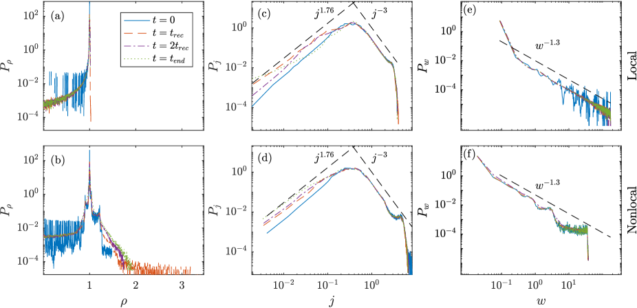
Figure 4: Plots of the probability density functions (PDF) of various hydrodynamical quantities, in the local (left) and non-local (right) models. (a,b): PDF of the superfluid densities $|\psi|^{2}$. High density events $\rho>1$ are well represented in the non-local case (b), whereas they are absent in the local model (a). (c,d): PDF of the probability current norm $j=\left|{\mbox{\boldmath$j$}}\right|$ (see text for a precise definition). A $j^{-3}$ behavior is observed on the right tails of both models and comes from the midrange decay of $j$. A $j^{1.76}$ scaling is observable on both left tails. (e,f): PDF of the pseudo-vorticity norm $w=\left|{\mbox{\boldmath$w$}}\right|$ (Eq. 8). The observed power-law behaviors $P_{w}\sim w^{-1.4}$ are super-imposed in both the local and non-local cases.

To quantify more precisely the generation of strong fluctuations of the superfluid density $\rho=|\psi|^{2}$, we compute the probability density function (PDF) of the field of densities obtained in the simulation domain for both the local and non-local cases, at the four times considered in Fig. 3, and we display our results in Figs. 4 (a) and (b). We observe that along the phenomenon of reconnection, densities higher that the uniform one are forbidden in the local case (Eq. 10). On the contrary, in the non-local approach, in which local densities higher than one are initially present due to the roton minimum, the dynamics may develop local mass concentration exceeding three times the value of the uniform density.

In order to interpret subsequent PDFs that we are going to estimate, let us first focus on the simple axisymmetric stationary solution (i.e. the vortex line) that we presented in Fig. 1 (d). Consider then any physical quantity of interest $F$, and its respective PDF $\mathcal{P}_{F}$, i.e. the histogram of the values $g(x,y,z)$ taken by the quantity $F$ in the domain $\mathcal{V}$ (of volume $|\mathcal{V}|$). The PDF can be written as the following empirical average

$$\mathcal{P}_{F}(f)=\frac{1}{|\mathcal{V}|}\int_{\mathcal{V}}\delta\left(f-g(x,y,z)\right)dxdydz,$$ (11)

where $\delta$ denotes the Dirac function. For a single vortex, in a cylindrical volume $\mathcal{V}$ of radius $R$ and of finite height, the PDF of $v$ can be computed exactly, inserting $g(r,\theta,z)=1/r$ in the empirical interpretation of the PDF (Eq. 11) and performing a proper change of variable, we get $\mathcal{P}_{|{\mbox{\boldmath$v$}}|}(|{\mbox{\boldmath$v$}}|)=2R^{-2}|{\mbox{\boldmath$v$}}|^{-3}$ for $|{\mbox{\boldmath$v$}}|\geq R^{-1}$ (and 0 for $|{\mbox{\boldmath$v$}}|<R^{-1}$), showing that the tail is governed by the divergence of velocity in the vicinity of the vortex, as it was noticed in Ref. Paoletti et al. (2008); Proment et al. (2012). Note that similar power-law behavior $\sim|{\mbox{\boldmath$v$}}|^{-3}$ have been observed in simulations of the local GP equation (Eq. 10) as detailed in Ref. White et al. (2010). This power-law behavior of the tail of the PDF of the norm of velocity is also observed for the case of two perpendicular vortices, as we consider to initiate our numerical simulations. We have checked in our simulation that this is also the case for the initial condition we are using, for both the local and non-local case, all long the reconnection process (data not shown).

To this regard, as we have already seen, the probability current field $j$ remains bounded in the presence of a vortex line, and thus appears to be a good candidate in order to quantify whether high values of density, as they are observed in particular in the non-local case (Fig. 4 (b)), are associated to high values of the current $j$. We display in Figs. 4 (c) and (d) the histograms of the values taken by the norm of the current vector $j$ in the computational domain. We see in both local and non-local cases, that the PDF of $|{\mbox{\boldmath$j$}}|$ exhibits similar tendencies, such as (i) a linear trend for $|{\mbox{\boldmath$j$}}|\ll 1$, and (ii) a $|{\mbox{\boldmath$j$}}|^{-3}$ power-law behavior in a domain of finite extension, reminiscent of the expected power law of the velocity field PDF, as explained formerly. The power law behavior at small $|{\mbox{\boldmath$j$}}|$ should be a consequence of the interaction of vortices and their images, and the finiteness of the extension of the computational domain (and the respective periodical boundary condition). Even if higher values of the current field $|{\mbox{\boldmath$j$}}|$ are indeed observed in the non-local case (Fig. 4 (d)), they do not exceed values already observed in the initial condition at $t=0$. We are lead to the conclusion that the existence of a roton minimum has little influence on the overall shape of the PDFs of $|{\mbox{\boldmath$j$}}|$.

Developing on these ideas, we perform a similar estimation of the histogram of the pseudo-vorticity $w$ (Eq. 8), in order to quantify possible creation of small scales, as it happens in the presence of a direct cascade mechanism, which is at the heart of the phenomenology of Kolmogorov regarding three-dimensional classical (i.e. governed by the viscous Navier-Stokes equation) turbulence Frisch (1995). Indeed, recall that in classical turbulence, velocity PDF is close to a Gaussian function, whereas PDF of gradients, and in particular vorticity, is found highly non Gaussian. For a vortex line along the $z$-axis, we know well that pseudo-vorticity is expected to be a bounded vector, taking significant values only for $r$ of the order and smaller than $a$. Using thus the schematic distribution provided in Eq. 9, it is easy to get, from Eq. 11, that we expect $\mathcal{P}_{|{\mbox{\boldmath$w$}}|}(|{\mbox{\boldmath$w$}}|)\propto|{\mbox{\boldmath$w$}}|^{-1-\alpha^{-1}}$. This assumption on the radial profile of pseudo-vorticity allows to reproduce the present observed histograms of the values taken by $|{\mbox{\boldmath$w$}}|$ in our simulation domain at any time of the reconnection process, as it is displayed in Figs. 4 (e) and (f). According to this model, using $\alpha\approx 3.125$ for both the local and non-local cases, we expect a power law decrease of the PDF with an exponent $\approx 1.3$, as it is presently observed. As we mentioned formerly, for a single stationary vortex, the large $r$ asymptotic for the pseudo-vorticity gives $|{\mbox{\boldmath$w$}}|\propto r^{-4}$, which suggests $\alpha=2$. It gives a different power law exponent for the PDF of $|{\mbox{\boldmath$w$}}|$, namely $|{\mbox{\boldmath$w$}}|^{-1.5}$ instead of our observed $|{\mbox{\boldmath$w$}}|^{-1.3}$ behavior. Once again, this difference could be explained by the fact that the PDF that is measured here is for two vortices during reconnection in a finite periodic domain, contrary to the large $r$ asymptotic that is derived for a single, straight vortex in infinite space.

We would like now to comment briefly on the amount of sound emitted following the reconnection event. Such a study has been carried out in the literature using the local formulation of the GP equation (Eq. 10) Nore et al. (1997); di Leoni et al. (2017), that we repeat here for the nonlocal version. Decomposing the conserved total energy as the sum of various components, we identify the part associated to kinetic energy as being the average (over space and time, the time integration starting at $t_{rec}$ until the end of the simulation) of the norm square of the vector $\sqrt{\rho}{\mbox{\boldmath$v$}}$, a vector field being itself decomposed into a divergence-free part (i.e. incompressible) and a compressible part, a decomposition easily performed in the Fourier space. Doing so, we obtain, in average, the incompressible $E_{\text{kin}}^{\text{i}}$ and compressible $E_{\text{kin}}^{\text{c}}$ kinetic energies. In present numerical simulations, we obtain for the ratio $E_{\text{kin}}^{\text{c}}/E_{\text{kin}}^{\text{i}}$ of these energies a value of $0.045$ in the local case, and $0.073$ for the non local version. Although more sound is emited in the non local case, overall it shows that the most part of the kinetic energy is held by the incompressible motions.

This being said, even if there are some differences implied by the existence of the roton minimum, we are led to the conclusion that there is no creation of small scales, i.e. no creation of high value of pseudo-vorticity, even in the presence of a model taking into account a realistic picture of the core of vortices. We will come back to this point in the conclusion.

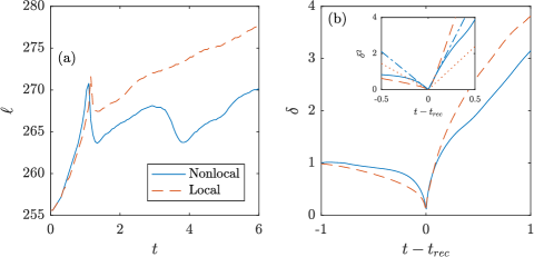
Figure 5: (a): Total length of the set of two vortices (see text), in the local (red) and non-local (blue) models. (b): Distance $\delta$ between the two vortices, in the local (red) and non-local (blue). Inset: squared distance $\delta^{2}$ between the two vortices for both models and their respective linear fit (dashed and dotted-dashed lines). The slopes of the linear fits before and after reconnection are given in the text.

VII Tracking vortices

Let us now explore some other aspects of the vortex reconnection process, as those related to the evolution of vortices as individual objects. Such kind of studies rely on the tracking of vortex cores, i.e. regions of space where density vanishes. This can be done using algorithms that seek zeros in planes, in order to extract lines in three-dimensional space with the help of the pseudo-vorticity, as it is proposed in recent literature Villois et al. (2016). In this section, we revisit what has been done in this context for the local GP equation Rorai et al. (2016); Villois et al. (2017); Zuccher et al. (2012), and in experiments Fonda et al. (2014), and compare with what is obtained in the non-local case. In few words, this numerical tracking algorithm provides the position vector ${\mbox{\boldmath$X$}}(s,t)$ at each time $t$ and parameterized by the length $s$ measured along the filament made of the points that do not hold a density. From there, we can define the Frenet-Serret frame of reference, given by the orthonormal set of vectors $({\mbox{\boldmath$T$}},{\mbox{\boldmath$N$}},{\mbox{\boldmath$B$}})$, where ${\mbox{\boldmath$T$}}=\partial{\mbox{\boldmath$X$}}/\partial s$ is the tangential vector, ${\mbox{\boldmath$N$}}=(\partial{\mbox{\boldmath$T$}}/\partial s)/|\partial{\mbox{\boldmath$T$}}/\partial s|$ the normal vector, and ${\mbox{\boldmath$B$}}={\mbox{\boldmath$T$}}\wedge{\mbox{\boldmath$N$}}$ the binormal vector. In a equivalent way, we could have introduced in the definition of this frame the curvature $\kappa(s,t)=|\partial{\mbox{\boldmath$T$}}/\partial s|$ and torsion $\tau(s,t)=-{\mbox{\boldmath$N$}}\cdot\partial{\mbox{\boldmath$B$}}/\partial s$, where $\cdot$ stands for the scalar product (see Ref. Hasimoto (1972) for instance).

In subsequent developments, we will analyze the vortex reconnection phenomenon in the Frenet-Serret frame, and compare with the well-known schematic model given by the local induction approximation (LIA). LIA has been studied for a long time in various aspects of fluid dynamics, and can be derived in a systematic way from the Navier-Stokes equation Callegari and Ting (1978) assuming that the vortex core size is small compared to some characteristic curvature. From a dynamical point of view, this approximation implies that the time variation of the position ${\mbox{\boldmath$X$}}(s,t)$ for some time independent parameterization $s$ has only a contribution along the binormal vector, namely $\dot{{\mbox{\boldmath$X$}}}=\partial{\mbox{\boldmath$X$}}(s,t)/\partial t=G\kappa(s,t){\mbox{\boldmath$B$}}(s,t)$, where $G$ is a constant that diverges logarithmically with the vortex core size, and $\kappa(s,t)$ the local curvature. The LIA predicts in a consistent way that indeed the length of such a vortex is conserved, and that solitary waves (i.e. solitons) can propagate at a constant speed Hasimoto (1972). Let us then compare these predictions against the dynamics of the reconnection process that we observe in our numerical estimations of the local and non-local GP equations.

We display in Fig. 5 (a) the length of the system made up of the two vortices, as they are displayed in Fig. 3. We furthermore include in the estimation of their lengths their copies in the whole simulation domain. Remark that the aforementioned tracking algorithm provides in a straightforward manner their lengths. We see that in both local and non-local cases, before reconnection, vortices undergo stretching, that make their length increases of a small amount (of order $5\%$) before decreasing. It follows then, after reconnection, a monotonic increase for the local case, and a more complex evolution for the non-local case. As we claimed, LIA predicts that the length is a constant a motion. Indeed, defining the length of a vortex as $\ell(t)=\int|\partial{\mbox{\boldmath$X$}}(s,t)/\partial s|ds$, we get from a general point of view (for any parameterization $s$) that $d\ell(t)/dt=\int\partial\dot{{\mbox{\boldmath$X$}}}/\partial s\cdot{\mbox{\boldmath$T$}}ds$, showing that a non vanishing component of the induced velocity $\dot{{\mbox{\boldmath$X$}}}$ along the normal vector $N$ may contribute to a variation of the length $\ell$, which is not the case in the LIA (only a component along the binormal is considered). Such arguments on vortex length have been rigorously studied in Klein and Majda (1991). As we can see in Fig. 5 (a), the length of vortices depends on time, a feature that is not allowed in the LIA, although only $5\%$ of the length undergo changes.

To carry on the description of the dynamical features of reconnection, we compute the distance separating vortices before and after reconnection, which is defined at each time as the minimum distance between two points on the two vortex lines. Such a numerical study has been performed systematically for the local GP equation for various initial conditions Villois et al. (2017), and it was found that this distance behaves as $|t-t_{\text{rec}}|^{1/2}$, both before and after reconnection. The square-root behavior can be understood using a linear approach, justified close to the vortex core (where density vanishes) Nazarenko and West (2003), or from a dimensional point of view (see for instance Ref. Hormoz and Brenner (2012)). The proportionality constant to this square-root law was found to depend on initial conditions, whether, as an example, vortices are taken perpendicular of anti-parallel. We represent in Fig. 5 (b) the time evolution of this distance $\delta$ before and after reconnection in our present numerical simulations (see also a representation of $\delta^{2}$ in the inset). For both the local and non-local cases, we reproduce the square-root behavior close to the reconnection time $t_{\text{rec}}$, but with slightly different proportionality constants. This numerical estimation shows that the roton minimum has here some influence, in particular we see that approaching and separation distances have different time evolution. The numerical values we observe for the proportionality constant in the local case (resp. nonlocal) are significantly different from the values observed in ref. Villois et al. (2017). We find $0.23$ (before reconnection) and $0.38$ (after reconnection) as far the local case is considered. Concerning the nonlocal case, we find $0.33$ (before $t_{\text{rec}}$) and $0.81$ (after $t_{\text{rec}}$). We recall that it was found in Ref. Villois et al. (2017), for the local case, the corresponding values $0.55$ and $0.63$. Remark that, in this study, the two orthogonal vortices are initially separated by an atomic distance $a$, whereas this initial distance was chosen to be six healing lengths (which is of the same order of $a$), thus a factor of order 6 for the chosen initial separations. This could explain once again the strong dependence of this multiplicative constant on initial conditions, and the differences in between the present numerical study and the one proposed in Ref. Villois et al. (2017). However it is worth noticing that even if we observe slightly different values of the proportionnality constants in the local model, in both our case and the observation of Ref. Villois et al. (2017) the value of the constant after the reconnection is always greater than the value of the constant before reconnection.

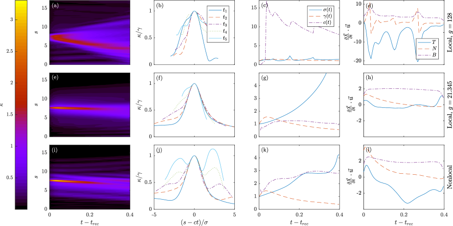
Figure 6: (a,e,i): space-time maps of the local curvature of a vortex line $\kappa(s,t)$, in the local case for $g=128$ (in (a)) and $g=21.345$ (in (e)), and for the non-local model (in (i)). The position of the principal curvature maximum is tracked along time. (b,f,j): corresponding curvature profiles of the tracked maximum at five regularly spaced times during its propagation. Each profile is scaled back onto the initial condition at reconnection. Snapshot times are $t_{1}=t_{\text{rec}}$, $t_{2}=t_{\text{rec}}+0.09$, $t_{3}=t_{\text{rec}}+0.17$, $t_{4}=t_{\text{rec}}+0.26$ and $t_{5}=t_{\text{rec}}+0.34$. We observe the growth of secondary curvature maxima in the non-local case (see (j)). (c,g,k): time evolution of the $\sigma$, $\gamma$, $c$ scaling parameters, which represent the width, height and velocity of the curvature wave packet respectively (see Eq. 12). (d,h,l): projections of the velocity vector of the local maximum of curvature onto the Frenet-Serret orthonormal basis $T$, $N$, $B$.

VIII Characterization of a propagating wave packet

Visualization of the overall reconnection phenomenon, as it is displayed in Fig. 3 suggests the creation of a localized phenomenon along the vortices. To exhibit this phenomenon quantitatively, we display in Fig. 6 maps of local curvature, i.e. the numerical estimation, thanks to the vortex tracking algorithm, of spatiotemporal maps of $\kappa(s,t)$ as a function of the arc-length $s$ and time $t$. We indeed observe in both the local and non-local cases the propagation of a wave packet of curvature, as it is predicted by the LIA, and conveniently formalized in Ref. Hasimoto (1972). As far as the local case is concerned, we study moreover two particular values for the interaction parameter $g$ entering in the dynamics (Eq. 10). As we have seen in Section VI, $g$ governs in the same time the speed of sound (i.e. $c_{s}=\sqrt{2g}$) and the healing length (i.e. $\xi=1/\sqrt{g}$) once is chosen $g=\mu$ as it is done in Eq. 10. Thus, speed of sound is inversely proportional to the healing length. In our situation, the value $g=128$ (the respective curvature map and related quantities are displayed in Figs. 6(a) to (d)) ensures a same speed of sound as in the non local version (Eq. 1), but with a vortex core diameter smaller than what is obtained in the model with rotons (see in particular Fig. 2(b)). We also study the value $g=21.345$ (displayed in Figs. 6(e) to (h)) for which vortex core size is similar to the nonlocal case (data not shown) but with a smaller speed of sound. Respective results concerning the non local case are displayed in Figs. 6(i) to (l). As we will see in the following, the propagation of a wave packet is clear in the $g=21.345$ and in the non local cases, whereas it is less clear in the $g=128$ case. This might be due to the smallness of vortex cores that makes them stiff and somehow imposes a much higher speed of propagation of the wave packet, which turns out to be difficult to track. Remark first that indeed, the wave packet, and in particular the local maximum of curvature (i.e. bright colors), seems to propagate approximately at a constant speed i.e. $c=ds/dt$, for both the local and non-local cases, although in the non-local case, secondary maxima appear during the propagation.

To quantify more accurately the wave packet velocity and its shape in the vicinity of the curvature maximum, we display in Figs. 6 (b), (f) and (j) a tentative rescaling of the observed curvature at various instants as

$$\gamma(t)\kappa\left(\frac{s-c(t)t}{\sigma(t)},t\right),$$ (12)

where $c(t)$ is the velocity of the maximum of curvature, $\sigma(t)$ a typical length quantifying the increase in the width of the wave packet, and $\gamma(t)$ that allows to include a possible time-variation in the amplitude. We indeed observe that this rescaling procedure makes the curvature profile similar to what is observed initially. Under the LIA, it is shown in Ref. Hasimoto (1972) that such a wave packet is expected to behave as a solitary wave that propagates at a constant velocity (given by the initial torsion) and does not change neither its shape, nor its amplitude, i.e. $\sigma(t)=\gamma(t)=1$, the actual time independent shape being given by a hyperbolic secant function. In the sequel, we will mostly focus on the $g=21.345$ local case, and on the non local case, since for the $g=128$ local case, the propagation of the wave packet appears to be different, and compares poorly with predictions of LIA. In our present numerical simulation, we see that in a good approximation, except at early times ($t<0.1$), the velocity of the wave packet, $c(t)$, is nearly constant, of order $c\approx 1$ in the local case (Fig. 6(g)), and of order $c\approx 2$ (Fig. 6(k)) in the non-local one, as it is suggested in the LIA approach. In comparison, the celerity of sound in the superfluid is $c_{s}=16$ in these units: the observed wave packet propagates in a much slower way than acoustic waves, although in the local stiff case (Fig. 6(c)), the velocity of the wave packet may reach such values. On the contrary, the wave packet undergoes both dispersion, i.e. its width increases as tracked by the increase of the rescaling coefficient $\sigma(t)$, and its amplitude decreases, with accordingly a decrease in the coefficient $\gamma(t)$. A more precise analysis shows indeed that $\gamma(t)\sim 1/t$, a decrease that is not predicted by LIA.

Focusing on the local $g=21.345$ and non local cases, in order to interpret these observed behaviors, we display in Figs. 6 (h) and (l) the projections of the vortex velocity vector $\partial{\mbox{\boldmath$X$}}/\partial t$ in the Frenet-Serret frame of reference $({\mbox{\boldmath$T$}},{\mbox{\boldmath$N$}},{\mbox{\boldmath$B$}})$ as a function of time. We indeed observe that the projection along the binormal vector is constant during the wave packet propagation, as it is assumed in the LIA. Let us precise here that if indeed the projection of $\partial{\mbox{\boldmath$X$}}/\partial t$ on $B$ appears to be time independent, we can infer from the tracking of the wave packet itself (Figs. 6 (h) and (l)) that the actual value of this projection cannot be given by only the curvature since curvature itself is found dependent on time. Interestingly, at early stage following reconnection, once again for $t<0.1$, we see a non vanishing contribution along the normal vector $N$. As shown in Ref. Klein and Majda (1991), this part of the dynamics is involved in a self-stretching phenomenon that would modify the length of vortices, as it is indeed observed in Fig. 5 (a). As time evolves, this projection gets smaller and smaller. Finally, we see that in the local case, the projection along the tangential vector $T$ is always negligible in front the projections along the other direction of the frame, whereas it cannot be neglected in the non-local case. This might be explained while studying the interaction with additional local maxima that appear during the wave packet propagation for the non-local case. Returning to the stiff $g=128$ local case (Fig. 6 (d)), once again we see that the projection on the binormal vector remains also constant, and the projection on the normal vector remains negligible. On the contrary, the projection on the tangential vector may take large negative values, a phenomenon that remains to be understood. Let us mention again that since the wave packet travels very fast, it is difficult to track and the strong variations observed on the projection along the tangent vector may be due to the existence of several packets which interact in a complicated way.

IX Conclusion and final remarks

We have studied numerically the reconnection phenomenon of two initially orthogonal quantum vortices in a model of superfluids which includes the roton minimum in the dispersion relation. As it was proposed in the literature Pomeau and Rica (1993); Berloff and Roberts (1999); Berloff (1999), such a model describes the dynamics of a scalar wave function that is governed by the Gross-Pitaevskii equation Pitaevskii and Stringari (2003) where is considered a non-local two-body interaction of characteristic extension the ${}^{4}\mathrm{He}$ atomic size $a$. We start by calibrating the model to be as close as possible to the experimental dispersion relation of ${}^{4}\mathrm{He}$ provided in Ref. Donnelly and Barenghi (1998), with the additional will to prevent from the generation of precursors of crystallization, as it was evidenced in Ref. Berloff (1999), although of great importance in the context of supersolidity Pomeau and Rica (1994); Josserand et al. (2007). Once obtained such a model, we estimate its stationary vortex solution, that is a time independent solution with an axis symmetry, around which the phase turns of an angle equals to 2$\pi$. Then, in a similar way as in Ref. Koplik and Levine (1993), we prepare a initial condition made up of two of these vortices in a orthogonal situation. We indeed observe a reconnection, and track and study the time evolution of the density, current and pseudo-vorticity fields, we provide both a statistical analysis of the fields and a local estimation of the geometry of these vortices, including a precise characterization of a observed wave packet that shares some features predicted by the LIA.

This numerical investigation shows that taking into account a more realistic structure of vortices, as depicted in Ref. Villerot et al. (2012), has little influence on the global picture of reconnection given by the local version of the GP equation and presented in Ref. Koplik and Levine (1993), although the creation and propagation of a wave packet of curvature along the vortex cores appear more complex when the non-local interaction is plugged in the dynamics.

The statistical analysis of the kinematic quantities involved in the dynamics, in particular current $j$ and pseudo-vorticity ${\mbox{\boldmath$w$}}={\mbox{\boldmath$\nabla$}}\wedge{\mbox{\boldmath$j$}}$, shows that there is no creation of scales smaller that the injected atomic length size $a$. This makes a big difference with what is obtained with the incompressible Euler or Navier-Stokes equations, where a cascading phenomenon transfers energy towards the small scales, as recently put in evidence while considering two colliding vortex rings in a experimental (classical) flow Mc Keown et al. (2018). We can thus infer that the hydrodynamics implied by the local and non-local versions of the GP equations, because of its implied high level of compressibility in the vicinity of the vortices, and the unclear action of the additional quantum pressure term, is indeed very different from the one of incompressible viscous Newtonian fluids.

It would of tremendous importance to develop an interaction term in the GP evolution of the wave function able to include a more realistic prediction of the dispersion relation, without exhibiting crystallization phenomena that are not expected in the superfluid phase of ${}^{4}\mathrm{He}$. We keep this perspective for future investigations.