Modelling mid-infrared molecular emission lines from T Tauri stars

We introduce a new modelling framework including the Fast Line Tracer (FLiTs) to simulate infrared line emission spectra from protoplanetary discs. This paper focusses on the mid-IR spectral region between 9.7 $\mu$m to 40 $\mu$m for T Tauri stars. The generated spectra contain several tens of thousands of molecular emission lines of H₂O, OH, CO, CO₂, HCN, C₂H₂, H₂, and a few other molecules, as well as the forbidden atomic emission lines of S I, S II, S III, Si II, Fe II, Ne II, Ne III, Ar II, and Ar III. In contrast to previously published works, we do not treat the abundances of the molecules nor the temperature in the disc as free parameters, but use the complex results of detailed 2D ProDiMo disc models concerning gas and dust temperature structure, and molecular concentrations. FLiTs computes the line emission spectra by ray tracing in an efficient, fast and reliable way. The results are broadly consistent with $R\!=\!600$ Spitzer/IRS observational data of T Tauri stars concerning line strengths, colour, and line ratios. In order to achieve that agreement, however, we need to assume either a high gas/dust mass ratio of order 1000, or the presence of illuminated disc walls at distances of a few au, for example due to disc-planet interactions. These walls are irradiated and heated by the star which causes the molecules to emit strongly in the mid-IR. The molecules in the walls cannot be photodissociated easily by UV because of the large densities in the walls favouring their re-formation. Most observable molecular emission lines are found to be optically thick. An abundance analysis is hence not straightforward, and the results of simple slab models concerning molecular column densities can be misleading. We find that the difference between gas and dust temperatures in the disc surface is important for the line formation. The mid-IR emission features of different molecules probe the gas temperature at different depths in the disc, along the following sequence:  OH (highest)  –  CO  –  H₂O and CO₂  –  HCN  –  C₂H₂ (deepest),  just where these molecules start to become abundant. We briefly discuss the effects of C/O ratio and choice of chemical rate network on these results. Our analysis offers new ways to infer the chemical and temperature structure of T Tauri discs from future James Webb Space Telescope (JWST)/MIRI observations, and to possibly detect secondary illuminated disc walls based on their specific mid-IR molecular signature.

1 Introduction

The Spitzer Space Telescope was the first astronomical instrument to detect water and simple organic molecules in protoplanetary discs at mid-IR wavelengths. Lahuis et al. (2006) reported on absorption bands of CO₂, HCN and C₂H₂ in the spectrum of the embedded low-mass young stellar object IRS 46, attributed to molecules in the line of sight within a distance of few au from this embedded star. Further early detections from Spitzer concerned the mid-IR H₂ lines (Nomura & Millar, 2005) and the [Ne II] 12.81 $\mu$m line (Pascucci et al., 2007; Güdel et al., 2010), the latter showing slightly blue-shifted profiles in follow-up VISIR high-spectral resolution observations by Pascucci & Sterzik (2009), interpreted as evidence for a slow disc wind. Other forbidden lines were detected by Baldovin-Saavedra et al. (2011), in particular [Fe II] lines, whereas [Ne III] and [S III] were not found.

The detection of mid-IR H₂O lines by Spitzer/IRS was announced simultaneously by Carr & Najita (2008) for AA Tau and by Salyk et al. (2008) for DR Tau and AS 205. A rich variety of H₂O and OH molecular line emission features were observed in addition to some of the already detected molecules and ions listed above. Pontoppidan et al. (2010b) re-reduced archival Spitzer/IRS spectra and established that the majority of T Tauri stars show water emission features in the $10-36\,\mu$m spectral range, originating from the $0.1-2$ au radial disc region with characteristic emission temperatures of about $300-1000$ K. This analysis was generally confirmed later by Salyk et al. (2011) and Carr & Najita (2011).

The analysis of the emission lines of TW Hya by Najita et al. (2010) revealed strong OH lines, in particular at longer wavelengths $\sim\!20-36\,\mu$m, and high-excitation HI lines such asHI (9-7) at 11.31 $\mu$m and HI (7-6) at 12.37 $\mu$m. Rigliaco et al. (2015) carefully re-reduced a large number of $R\!=\!600$ Spitzer/IRS spectra of T Tauri stars. These authors concluded that the hydrogen lines do not trace the gas in the disc, but rather the gas accreting onto the star in the same way as other hydrogen recombination lines do at shorter wavelengths.

Pascucci et al. (2009, 2013) reported on variations of the C₂H₂ and HCN line strengths with stellar spectral type. Najita et al. (2013) related the HCN/water ratio to the carbon to oxygen (C/O) element abundance ratio. One current interpretation is that the C/O ratio might be considerably larger than solar in the planet-forming region of protoplanetary discs, varying with stellar type and varying between individual objects (e.g. Du et al., 2015; Kama et al., 2016; Walsh et al., 2015). However, high-resolution optical spectra of Herbig Ae stars show that the C/O ratio of the gas that is accreted onto the stars always has the same, solar-like value (Folsom et al., 2012; Kama et al., 2015). An interesting observation is the detection of the C₂H₂ emission feature at 13.7 $\mu$m in some T Tauri stars because at solar C/O this molecule should only be abundant in deeper layers that are already optically thick in the continuum (Agúndez et al., 2008; Walsh et al., 2015). However, this conclusion depends on our possibly incomplete understanding of the warm chemistry in discs, and mixing processes could increase the concentrations of such molecules in upper, observable disc layers (Semenov & Wiebe, 2011).

Herbig Ae/Be stars show much lower detection rates of mid-IR molecular emission lines with Spitzer/IRS in comparison to T Tauri stars, in the form of tentative detections of H₂O and OH beyond 20 $\mu$m (Pontoppidan et al., 2010b) only in a few cases. It has been suggested that the missing water lines could be caused by some specific chemical or excitation effects in the warmer Herbig Ae discs (Meijerink et al., 2009; Fedele et al., 2011) or by growing inner cavities (Banzatti et al., 2017). However, these lines are also buried in a stronger continuum. Antonellini et al. (2016) have argued that common data reduction techniques, such as pattern noise and de-fringing, are likely to produce higher noise levels when the continuum is stronger. Therefore, the Spitzer observations might have been simply not deep enough to detect a similar level of mid-IR molecular emission from Herbig Ae/Be stars.

Simple slab models have been used in most cases for the analysis of these data in terms of molecular column densities and disc temperatures. In these slab models, a single temperature and fixed molecular concentrations are considered, and the excitation of the molecules is approximated in local thermodynamic equilibrium (LTE). The integration along the line of sight can be solved analytically in this case, hence these models are actually single-point (0D) models, and the results only depend on the temperature and molecular column densities assumed. The solid angle of the emitting region is adjusted later to match the observed strength of the molecular emission features. However, these slab models come in a number of variants. The lines of different molecules from the same disc are often fitted with different physical slab-parameters. Also the way in which the dust continuum is treated in these models differs considerably among different authors. In the near and mid-IR, dust opacity effects are likely to be very important as large amounts of molecules are expected to be present below the $\tau_{\rm dust}=1$ surface where they do not produce any observable signatures.

The concept of LTE-slab models can be generalised to non-LTE, where again a single temperature and a single gas density is considered, for example the RADEX code (van der Tak et al., 2007). The molecular level populations are computed at given molecular column density using the escape-probability formalism, and background radiation fields in the form $J_{\nu}\!=\!WB_{\nu}(T_{\rm rad})$ can be included, an effect called radiative pumping. Like in LTE slab models, the integration along the line of sight can be solved analytically, but in addition to the temperature $T$ and the molecular column density, the non-LTE slab model results also depend on volume density, dilution factor $W$, and radiative temperature $T_{\rm rad}$.

Series of slab models can be used to better represent the changing physical conditions with radius along the disc surface, either assuming LTE or non-LTE, in particular for CO fundamental ro-vibrational emission (Blake & Boogert, 2004; Thi & Bik, 2005; Thi et al., 2005; Brittain et al., 2009; Ilee et al., 2013, 2014; Carmona et al., 2017). These models usually use power laws for molecular column densities and temperature as a function of radius. Such 1D slab models are then integrated over the radius to compute the total line emission fluxes from the disc.

Bruderer et al. (2015) compiled a non-LTE model for the HCN molecule from the literature for ro-vibrational levels. A combination of LTE and non-LTE slab models was performed, as well as a full 2D disc model of the T Tauri star AS 205 (N), which is well-known for its exceptionally strong molecular emission lines in the IR and far-IR spectral regions (Salyk et al., 2011; Fedele et al., 2013). However, Bruderer et al. did not use their own consistent results for gas temperature and molecular concentrations, but have chosen to assume $T_{\rm gas}\!=\!T_{\rm dust}$ and to introduce parameterised jump-abundances to avoid the complexity of heating/cooling balance and kinetic chemistry in discs for the interpretation of the spectra. These authors found a critical density for the population of the upper vibrational state of the HCN 14 $\mu$m feature of order $\sim\!10^{12}\rm\,cm^{-3}$, and concluded that non-LTE effects can increase the mid-IR line fluxes by up to a factor of about three. Concerning the hot 3 $\mu$m band of HCN, non-LTE effects can also cause extended emission, leading to more centrally peaked lines.

Similar investigations have recently been carried out by Bosman et al. (2017) for the CO₂ molecule in AS 205 (N). The authors found a critical density for the population of the upper vibrational level of the 15 $\mu$m CO₂ emission feature of $\sim\!10^{12}\rm\,cm^{-3}$ and arrived at similar conclusions about the importance of non-LTE effects. They also present first predictions for the IR spectrum of the ¹³CO₂ molecule in consideration of JWST. However, the assumption of $T_{\rm gas}\!=\!T_{\rm dust}$ and the parameterised jump-abundances are likely to produce new uncertainties. In particular, the parameterised abundance causes the molecules to be present already at very high altitudes, where densities are low, radiation fields are strong, and hence non-LTE effects are likely to be important, whereas in our disc models molecules such as CO₂ and HCN are only abundant in deeper layers in which densities are larger and non-LTE effects are less important.

In new investigations, based on full 2D ProDiMo thermochemical disc models, Antonellini et al. (2015) have shown that the mid-IR water lines are excited very close to LTE, originate from different radii with different temperatures, and are affected by stellar luminosity and various disc properties, such as dust opacities, stellar UV irradiation, dust/gas ratio, dust settling, and disc inner radius. The emission spectra calculated by Antonellini et al. (2015) use the vertical escape probability technique (see Appendix A), which is strictly valid only for face-on discs.

2 Purpose of this paper

In this paper, we run full 2D ProDiMo thermochemical disc models to predict the dust and gas temperature structures and molecular concentrations, and then perform a global ray-tracing technique to simulate the molecular emission lines from protoplanetary discs. We introduce FLiTs, the fast line tracer, to ray trace the entire disc for arbitrary inclination angles. For demonstration, we use this new modelling platform to simulate the entire line emission spectra of T Tauri discs in the mid-IR wavelength region, where the observational data contains a wealth of spectroscopically unresolved emission lines that merge into complicated spectral emission features. We convolve our high-resolution spectra to a spectral resolution of $R\!=\!600$ to compare the spectra to a small collection of Spitzer/IRS spectra of T Tauri stars from Rigliaco et al. (2015).

We do not intend to fit any particular observational data in this paper, but we want to discuss to what extent our model spectra are broadly consistent with the observed line strengths and spectral shapes of the emission features for various molecules. We investigate which disc properties are responsible for the strength and colour of line emission, including disc shape and dust opacities. We want to explore to what extent the chemical concentrations predicted by ProDiMo are consistent with the Spitzer/IRS data, or whether certain molecules are possibly underpredicted or overpredicted in systematic ways. We briefly discuss the underlying uncertainties in chemical rate networks and the carbon to oxygen ratio.

These are a few first steps towards solving the more important, general scientific questions connected to infrared line emission spectra from protoplanetary discs.

• What is the molecular composition of the warm gas in the planet-forming regions of protoplanetary discs?

• Why do some T Tauri stars show strong molecular emission lines whereas others do not? Why do Herbig Ae stars show lower detection rates?

• What are the principal chemical and physical processes to excite the molecular emission lines, and how tightly are these related to stellar properties such as UV excess and X-ray luminosities?

• Can we infer the vertical gas temperature structure in the planet-forming region from the observation of IR molecular emission lines?

• Can we use IR molecular emission lines to diagnose disc winds and disc shape anomalies such as gaps, vortices, and spiral waves at radial distances of a few au?

• What can we conclude about dust opacities and disc evolution in the planet-forming region of protoplanetary discs?

• What are the predictions for JWST/MIRI in the near and SPICA/SMI in the distant future, which new science questions can we address, and what are the prospects of discovering new molecules at IR wavelengths?

• Is there evidence for an enrichment of the gas with elements outgassing from comets/pebbles that migrate inwards? Can this process cause a carbon-rich local environment?

Archival (e.g. Spitzer/IRS) and future observational spectra (e.g. JWST/MIRI, in the distant future SPICA/SMI) will contain valuable information about the physico-chemical state of protoplanetary discs in the planet-forming regions as probed by mid-IR line emission, but in order to deduce this information from the data and to address the questions above, we need to go beyond simple isothermal slab models in LTE. We require disc models that include a detailed treatment of the disc structure, dust radiative transfer, gas heating and cooling, chemistry, and line radiative transfer.

The future JWST/MIRI data will improve by a factor of about five in spectral resolution and will have a sensitivity significantly higher than the current Spitzer/IRS data. However, for JWST/MIRI, we still have to face the challenge of analysing spectrally unresolved data. To assist with the correct interpretation and to address special questions concerning the dynamics of gas and winds, follow-up observations at high spectral resolution ($R\!\ga\!17000$) are required. Such observations have been carried out using ground-based near-IR and mid-IR spectrographs such as the Very Large Telescope (VLT)/CRIRES (Thi et al., 2013; Carmona et al., 2014), VLT/VISIR (Pontoppidan et al., 2010a; Pascucci et al., 2011; Baldovin-Saavedra et al., 2012; Sacco et al., 2012; Banzatti et al., 2014), GEMINI/TEXES (Salyk et al., 2015) or GEMINI/MICHELLE (Herczeg et al., 2007). The ProDiMo models have already been used successfully to interpret high-resolution near-IR data (e.g. Hein Bertelsen et al., 2014, 2016b, 2016a), and the new ProDiMo $+$ FLiTs models introduced in this paper are expected to provide an excellent basis to analyse high-resolution mid-IR data in the future. However, in this paper, we concentrate on discussing the spectrally unresolved Spitzer/IRS data and future prospects for JWST/MIRI.

3 Disc model

To simulate the mid-IR emission line spectra from T Tauri stars, we use the radiation thermochemical disc models described by Woitke et al. (2016). The models are based on MCFOST (Pinte et al., 2006) and MCMax (Min et al., 2009) Monte-Carlo radiative transfer coupled to disc chemistry, gas heating and cooling balance, and non-LTE line formation performed by ProDiMo (Woitke et al., 2009; Kamp et al., 2010; Thi et al., 2011). In this paper, we use a generic model set-up for a T Tauri disc as described in (Woitke et al., 2016). A protoplanetary disc of mass $0.01\,$M_⊙ is considered around a K7-type young star of mass $M_{\star}=0.7\,$M_⊙ and stellar luminosity $L_{\star}=1\,$L_⊙, with an age of about $1.6\,$Myrs at a distance of 140 pc. The disc is seen under an inclination of $45^{\circ}$. The disc is assumed to start at the dust sublimation radius of $R_{\rm in}\!=\!0.07$ au. Further disc shape and dust opacity parameters of this model are listed in (Woitke et al., 2016, see Table 3 therein).

In the main model selected for our broad comparison to Spitzer/IRS observations in this paper, however, we increased the gas/dust mass ratio (at constant dust mass) from 100 to 1000 to reach the observed strengths of the various line emission features. This idea was first introduced by Meijerink et al. (2009), modelling H₂O lines, and then later also used by Bruderer et al. (2015) and Bosman et al. (2017). Gas/dust ratios of order 1000 can readily be obtained in evolutionary disc models that take into account dust migration, for example after about 1 Myrs in the models of Birnstiel et al. (2012), as shown by Greenwood et al. (in prep.). The actual disc gas mass of the main model would therefore actually be $0.1\,$M_⊙. However, since the mid-IR lines originate well inside of 10 au, we only need to apply this modification to those regions, which does not reflect on the overall disc mass as only about 10% of the mass resides in those inner regions. Alternative ideas for how to increase the mid-IR line strengths (removal of small grains, e.g. by very strong dust settling, disc gaps with subsequent vertical walls) are briefly discussed in Sect. 6.3.

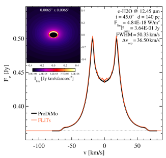
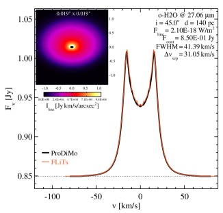
Figure 1: Computation of high-resolution single line profiles with ProDiMo (black lines) and FLiTs (red lines) based on a medium-resolution 90$\times$70 disc model. On the left side we show the o-H₂O rotational line $\rm 13_{\,6,5}\to 12_{\,4,9}$ at 12.453 $\mu$m with an excitation energy of 4213 K, which is emitted partly from the inner rim of the disc, and partly from the disc surface up to a radius of about 0.4 au in this model. On the right side, the o-H₂O rotational line $\rm 8_{\,5,4}\to 8_{\,2,7}$ at 27.059 $\mu$m is depicted, which has an excitation energy of 1806 K and is mainly emitted from the disc surface up to a radius of about 1 au. The time consumption is about 92 CPU-sec with ProDiMo ($251$ velocity-channels, $356\times 144$ rays) and 1.2 CPU-sec with FLiTs with enhanced accuracy settings (173 channels, 22375 rays), i.e. enhanced over FLiTs standards.

In the first modelling step, we calculated the opacities of the dust particles for sizes between $0.05\,\mu$m and $3\,$mm (see details in Min et al., 2016), considering about 100 dust size bins. A power-law size distribution was considered with constant dust/gas mass ratio throughout the disc, however in each column, we first computed the density-dependent settled size distribution according to Dubrulle et al. (1995), before summing up the total dust opacities at each point in the disc. We then perform a full 2D radiative transfer either by MCFOST, MCMax, or ProDiMo (can be used interchangeably) to obtain the dust temperature structure $T_{\rm dust}(r,z)$.

The disc model uses the large DIANA chemical standard with 235 gas and ice species (Kamp et al., 2017) and 90 heating and 83 cooling rates to compute the gas temperature and chemical concentrations at every point in the disc in local energy balance and kinetic chemical equilibrium. The level populations of the various atomic and molecular species are usually calculated in non-LTE in ProDiMo. However, with respect to previous publications, we included a few more ro-vibrational molecules from the HITRAN database (Rothman et al., 1998, 2013), approximating their level populations in LTE for simplicity. Table 3 summarises the relevant spectroscopic data in the mid-IR spectral region. Concerning the non-LTE atoms and molecules, an escape probability method is used to compute the level populations (Woitke et al., 2009), based on the calculated molecular column densities and continuum radiative transfer results. Thus, the IR-pumping of the level population by the emission and scattering of dust particles in the disc is fully taken into account. All spectral lines considered are automatically included as additional heating/cooling processes in ProDiMo.

We emphasise that we are using the full ProDiMo results in this paper (gas and dust temperatures, settled dust opacities, continuum mean intensities, chemical concentrations, and level populations) to compute the mid-IR molecular spectra of class II T Tauri discs if not otherwise stated, and this is different from Bruderer et al. (2015) and Bosman et al. (2017), for example.

The mid-IR line emitting regions in our disc model satisfy the physical condition of local energy conservation, which we consider as an advantage of our modelling approach. For example, the total line luminosity produced by these disc regions cannot exceed the total amount of energy that these regions receive from the star, either directly in the form of X-ray and UV photons triggering various heating processes, or indirectly via stellar photons that are processed by the disc to cause a strong local IR radiation field, which then heats the gas via line absorption. This is all taken into account in our model, which enables us to discuss, for example, how different disc geometries and different stellar irradiation properties produce different line emission spectra (see Sect. 6.4). Important heating and cooling processes in the line emitting regions are further discussed in Sect. 6.5.

4 FLiTs – the fast line tracer

The Fast Line Tracer (FLiTs) has been developed by M. Min to quickly and accurately compute the rich molecular emission line spectra from discs in the infrared, although it can principally be applied in all wavelength domains. It is a stand-alone Fortran-90 module designed to read the output from ProDiMo and perform the line ray tracing to simulate the observations of molecular line spectra.

The main challenges in this wavelength domain are (i) large numbers of molecular levels and lines, i.e. potentially tens of thousands of levels per molecule and millions of lines, for example known for H₂O and CH₄; (ii) physical overlaps of spectral lines, i.e. line photons emitted by one part of the disc may be absorbed in a different line by another part of the disc; and (iii) high optical depths in both line and continuum, which requires full radiative transfer solutions. Section 5 describes how a careful selection of molecules, levels, and lines can be made, while maintaining scientific significance, to bring the computational efforts down to a manageable level. In this section, we concentrate on the remaining technical challenges.

The basic equations and computational techniques used for line tracing are described in Woitke et al. (2011, see Appendix A7) and Pontoppidan et al. (2009). Pontoppidan et al. developed a similar line tracer called RadLite. Although we used some of the techniques and tricks described in their paper, we decided that our specific needs for speed and flexibility require a dedicated module for two reasons. First, we want it to be as fast and lightweight as possible. RadLite takes about one hour to compute 1000 lines (3.6 s per line); this is too long when fitting observations or making large grids of models. Second, RadLite traces on a line-by-line basis. This implies that we would not be able to compute line-blends self-consistently; see examples in Figs. 2 and 3. For this purpose, a new module was built from scratch that fulfils these requirements.

4.1 Numerical implementation

All physical quantities (i.e. dust opacities, dust source function with isotropic scattering, dust and gas temperatures, molecular concentrations, and non-LTE or LTE level populations) are passed from ProDiMo to FLiTs on the 2D spatial grid points used by ProDiMo. We assume Keplerian gas velocities, neglecting the effect of radial pressure gradients in the disc that typically slows down the rotation of the gas by a few percent in a power-law disc (e.g. Tazaki & Nomura, 2015). Pinte et al. (2018) have recently provided strong observational evidence that the disc of IM Lupi rotates with sup-Keplerian velocities beyond the tapering-off radius, where the column density decreases exponentially, but not at radial distances relevant to the IR molecular emission lines. In order to use the computational accelerations described in (Pontoppidan et al., 2009), we have to transform the point-based ProDiMo grid into a cell-based grid. Although we try to avoid interpolations as much as possible, this transformation can introduce some minor differences between the lines directly computed by ProDiMo and the lines computed by FLiTs.

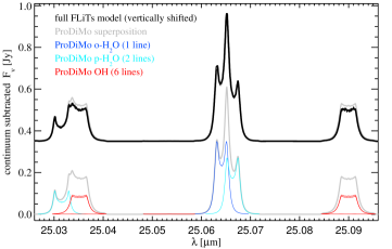
Figure 2: Computation of overlapping OH and H₂O lines with FLiTs and ProDiMo around 25 $\mu$m. The central feature shows two about equally strong water lines: o-H₂O (blue) $9_{7,2}\to 8_{6,3}$ at 25.0641 $\mu$m and p-H₂O (cyan) $9_{7,3}\to 8_{6,2}$ at 25.0663 $\mu$m. Although these two lines overlap spectroscopically, they do not overlap physically, and superposition (grey) still works fine in comparison to the full FLiTs model (black). On the right side, there are 3 individual OH lines (hyper-fine splitting) that physically overlap, $X_{3/2},v\!=\!0,J\!=\!12\!\to\!X_{3/2},v\!=\!0,J\!=\!11$ at 25.089950 $\mu$m (red, strong), $X_{3/2},v\!=\!0,J\!=\!11\!\to\!X_{3/2},v\!=\!0,J\!=\!10$ at 25.089946 $\mu$m (red, strong), and $X_{3/2},v\!=\!0,J\!=\!11\!\to\!X_{3/2},v\!=\!0,J\!=\!11$ at 25.089835 $\mu$m (red, very weak). The superposition gives slightly too strong results. On the left side, another case is shown with 1 p-H₂O line and 3 OH lines.

To calculate the line spectra, we integrate the monochromatic formal solution of radiative transfer for continuum $+$ lines along multiple parallel rays through the disc, at given inclination angle, for each wavelength. This way we construct an image of the disc at each wavelength (see Fig. 1). One of the crucial parts in this procedure is to avoid aliasing effects from the way the spatial or spectral grid are sampled. As we detail below, we avoid this aliasing by efficiently randomising the spatial and spectral sampling. This is very similar to using Monte Carlo integration techniques to integrate over the spatial extent of the disc and the finite width of a spectral bin.

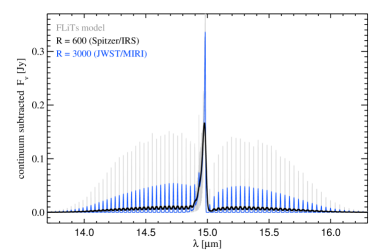
Figure 3: Pure CO₂ $\rm 01^{1}0(1)\to 00^{0}0(1)$ emission spectrum around 15 $\mu$m, showing the central $Q$-branch and the $P$ and $R$ side branches. On the left side, the full wavelength range is depicted; the grey line shows the original FLiTs spectrum, the black line shows the results convolved with a $R\!=\!600$ Gaussian, and the blue line the results convolved with a $R\!=\!3000$ Gaussian. The right plot shows a zoom into the $Q$-branch band-head, plotting only the original FLiTs spectrum. The individual lines have Keplerian double-peaked profiles, and merge with each other at maximum. At the band head, the total flux is smaller than expected from the sum of the individual $Q$-branch line fluxes because the lines physically overlap and partly shield each other in the disc.

In principle we need to carefully sample the physical line profile function given by thermal $+$ turbulent broadening, using a high enough spectral resolution. However, we created FLiTs in such a way that the model is also able to produce accurate results when running in significantly reduced spectral resolution. To do this, we do not sample each ray at exactly the same wavelength, but for each ray tracing through the disc we take a slightly different wavelength, randomly chosen within the wavelength bin considered. This way we randomly integrate over the finite width of the wavelength bin.

To increase the speed further, we store all computations done to avoid repeating the same work twice. This applies for example to the line profile function for each molecule at each location in the disc, and the continuum source function at each location and wavelength. At each velocity bin, the line contribution originates only from a very small region of the disc image. This means that we can reduce the computation time by finding exactly where that region is, and use the solution for the continuum ray tracing for the remaining disc image. For each parallel ray we store which cells are passed and what the projected velocity is. This way we know which rays contribute to which part of the observed line profile.

Table 1: Integrated line fluxes computed by FLiTs for the o-H₂O rotational line $\rm 13_{\,6,5}\to 12_{\,4,9}$ at 12.453 $\mu$m  [$10^{-18}$ W/m²]^(⋆)  as a function of velocity channel width $\Delta v$ and accuracy settings, based on the $140\times 140$ disc model.

Accuracy setting	$-1$ (lowest)	$1$ (default)	$5$ (highest)
$\Delta v=10$ km/s	$4.56\pm 0.48$	$4.80\pm 0.15$	$4.88\pm 0.07$
$\Delta v=5$ km/s	$4.81\pm 0.25$	$4.84\pm 0.06$	$4.86\pm 0.04$
$\Delta v=1$ km/s	$4.83\pm 0.04$	$4.86\pm 0.02$	$4.86\pm 0.003$

^(⋆): The numbers after $\pm$ denote the standard deviation of the line flux as estimated from a number of runs with different seeds for the random number generator. The results are consistent with ProDiMo ($4.84\times 10^{-18}$ W/m²); see Fig. 1.

4.2 Spatial sampling of the rays and accuracy

The most crucial part of the line radiative transfer is the spatial selection of ray positions and the underlying spatial resolution of the disc model. Each part of the disc is responsible for a different velocity component of the lines. We need to accurately sample the disc to resolve the line emitting regions at each wavelength, yet we have to make sure we do not oversample to avoid unnecessary computations. In FLiTs the disc is sampled by a bundle of parallel rays, the positions of which are determined by the projection of a number of random locations within each 2D disc model cell onto the image plane. Since the 2D disc model grid was set up to properly trace the temperature, density, and chemical variations in the disc, we now automatically sample this properly as well. The number of rays is determined by the accuracy settings in FLiTs. A larger accuracy number mean that more points per 2D disc model cell are projected onto the image plane, resulting in a better spatial resolution of the disc. Next we create a Delaunay triangulation from those selected points and use the centre of all triangles as ray positions. Since the positions of the rays are randomised this way, we avoid aliasing effects that would be visible when using relatively low resolution fixed spatial sampling. We also create a number of sets of ray positions and pick one of these for each wavelength to reduce the spatial sampling problems further.

Table 2: Time consumption of FLiTs in CPU sec / spectral line^(⋆) as a function of disc model grid size $N_{r}\times N_{z}$ and velocity channel width $\Delta v$.

model grid size	$50\times 40$	$90\times 70$	$140\times 140$	$200\times 300$
$\Delta v=5$ km/s	0.028	0.061	0.18	0.71
$\Delta v=2$ km/s	0.066	0.14	0.40	1.5
$\Delta v=1$ km/s	0.13	0.28	0.80	3.0
$\Delta v=0.5$ km/s	0.29	0.58	1.6	5.9

^(⋆): Tested on a 3.4 GHz Linux computer with accuracy$=\!-1$. The ‘accuracy’ setting in FLiTs determines how many rays are used to sample the disc, depending on the original ProDiMo disc model grid size. For the lowest accuracy level chosen here, FLiTs uses about 3000 rays for the $50\times 40$ model, 5000 rays for $90\times 70$, 7000 rays for $140\times 140$, and 12000 rays for $200\times 300$. For higher accuracy settings, more rays are used to better resolve the disc in the image plane.

In Fig. 1 we show a comparison of the computed single line profiles, demonstrating that the line profiles computed by ProDiMo are reproduced by FLiTs, with no systematic differences due to interpolation or numerics. Table 1 shows the computed line fluxes for one selected water line for various settings of spectral resolution and accuracy. The line fluxes computed by FLiTs show no systematic errors even for the lowest accuracy and poorest spectral resolution. However, higher accuracies are required to obtain precise line profiles as shown in Figs. 1, 2, and 3 (right side) to eliminate the noise introduced by the random spectral and spatial sampling.

Figure 3 represents how the superior signal-to-noise ratio and the improved spectral resolution of JWST/MIRI allows us for the first time to resolve individual $P$- and $Q$-branch lines of molecules like CO₂ in the mid-IR, and to use the ratios of those line fluxes as a thermometer, as already proposed by Bosman et al. (2017).

4.3 Computational time requirements

The computational time consumption of FLiTs depends on the accuracy and velocity resolution requested. Since the code is mainly developed for medium excitation ro-vibrational molecular lines with application to low spectral resolution observational mid-IR data, we do not need high accuracy nor velocity resolution for the subsequent models presented in this paper. Table 2 lists the computational time requirements of FLiTs when simulating a large number of lines with low accuracy setting. Noteworthy, the line fluxes obtained depend on the ProDiMo disc model grid size (see Appendix E in Woitke et al., 2016), which is related to the difficulty to spatially resolve the thin line forming regions; see Sect. 6.5. All results presented in Sect. 6 and beyond have been produced using $140\times 140$ disc models, FLiTs accuracy$\,=\!-1$ and $\Delta v\!=\!5\,$km/s, which corresponds to about 0.18 CPU-sec/line and a line flux error of about 5%. In contrast, the high spectral resolution results shown in Figs. 1 to 3 have been produced with accuracy $=\!+1$ and $\Delta v\!=\!1\,$km/s.

5 Selection of molecules, levels, and lines

Table 3: Selected atoms and molecules in the mid-IR spectral region.

	Treatment	$\lambda\rm\,[\mu m]$	#Levels(9)	#Lines	Reference
$\rm H_{2}O$	non-LTE	$2.3-600$	824	8190	(1),(2),(4)
$\rm OH$ rot.	non-LTE	$25-120$	20	50	(3),(8)
$\rm OH$ ro-vib.	HITRAN	$10-50$	2528	1264	(4)
$\rm CO_{2}$	HITRAN	$13-17$	252	126	(4)
$\rm HCN$	HITRAN	$12-17$	252	126	(4)
$\rm C_{2}H_{2}$	HITRAN	$11-16$	1992	996	(4)
$\rm NH_{3}$ ro-vib.	HITRAN	$9-50$	5932	2966	(4)
$\rm CH_{4}$	HITRAN	$18-25$	430	215	(4)
$\rm NO$	HITRAN	$28-50$	372	186	(4)
$\rm H_{2}CO$	HITRAN	$19-50$	3134	1567	(4)
$\rm CH_{3}OH$	HITRAN	$9-11$	28570	14285	(4)
$\rm SO_{2}$	HITRAN	$7-10$	41590	20795	(4)
$\rm H_{2}S$	HITRAN	$6-10$	1102	551	(4)
$\rm H_{2}$	non-LTE	$0.3-29$	160	1539	(6),(7)
$\rm Ne^{+}$	non-LTE	$0.4-12.81$	3	3	(5)
$\rm Ne^{++}$	non-LTE	$0.18-15.55$	5	9	(3)
$\rm Ar^{+}$	non-LTE	$6.985$	2	1	(3)
$\rm Ar^{++}$	non-LTE	$0.3-8.985$	5	9	(3)
$\rm Fe^{+}$	non-LTE	$0.2-25.99$	120	956	(5)
$\rm Si^{+}$	non-LTE	$0.1-34.81$	15	35	(5)
$\rm S$	non-LTE	$1.7-25.25$	3	3	(3)
$\rm S^{+}$	non-LTE	$0.4-31.45$	5	9	(5)
$\rm S^{++}$	non-LTE	$0.3-33.46$	5	9	(3)

(1) Faure & Josselin (2008); (2) Daniel et al. (2011); (3) LAMDA database (Schöier et al., 2005); (4) HITRAN 2009 database (Rothman et al., 1998, 2013); (5) CHIANTI database (Dere et al., 1997); (6) Wrathmall et al. (2007); (7) Lique (2015); (8) Offer et al. (1994); (9) for HITRAN molecules, the number of levels is by construction equal to $2\times$ the number of lines. Usually, all available levels and lines are included from the various databases, within the listed wavelength intervals. However, there are a few exceptions as follows:
OH ro-vib: levels with $E_{u}=900-30000\,$K only;
CO₂: only band $01101\to 00001$ and $E_{u}<5000\,$K;
HCN: only band $0110\to 0000$ and $E_{u}<5000\,$K;
NH₃: only band $0100\to 0000$ with $E_{u}=550-10000\,$K;
C₂H₂, CH₄, SO₂, H₂S: levels with $E_{u}<5000\,$K only;
NO, H₂CO, CH₃OH: levels with $E_{u}<10000\,$K only.

The selection of mid-IR active molecules and line lists for this paper is described in Table 3. We concentrate on molecules that have relevant line transitions between 9 $\mu$m and 40 $\mu$m. The extra heating/cooling rates caused by the absorption/emission of line photons by these species are automatically taken into account in ProDiMo. Other atomic and molecular species important for the radiative heating/cooling, for example those with fine-structure or pure rotational lines in the far-IR and at millimetre wavelengths, are included as well (see Woitke et al., 2009; Kamp et al., 2010; Woitke et al., 2011). But these other species are not explicitly listed in Table 3.

The new molecules include OH ro-vibrational, CO₂, HCN, C₂H₂, NH₃, CH₄, NO, H₂CO, CH₃OH, SO₂, and H₂S, for which we take the level energies, degeneracies, Einstein coefficients, line centre frequencies, and partition functions from the HITRAN database (Rothman et al., 1998, 2013). In this paper, we assume that the levels of these HITRAN molecules are populated in LTE, i.e. given by a Boltzmann distribution

$$n_{k}^{\rm LTE}=n_{\rm sp}\frac{g_{k}}{Q(T_{\rm gas})}\exp\bigg{(}-\frac{E_{k}}{kT_{\rm gas}}\bigg{)}\ ,$$ (1)

where $n_{\rm sp}$ is the total molecular particle density taken from the chemistry, $n_{k}\,\rm[1/cm^{3}]$ the level population, $g_{k}$ the level degeneracy, $E_{k}$ the level energy, and $Q(T)$ the partition function. $T_{\rm gas}$ is the gas temperature calculated in heating/cooling balance.

As we can handle only a few tens of thousands of spectral lines with ProDiMo and FLiTs, we need to select the relevant parts of the line lists in HITRAN, which originally contain many millions of transitions for a number of isotopologues. Our selection criteria are currently adjusted to the detections of the Spitzer Space Telescope, see Fig. 4, but this could easily be changed.

Our current selection of lines is restricted to particular vibrational bands and wavelength intervals, and only lines from the main isotopologues are taken into account; see details in Table 3. The following additional selection rule about the strength of the lines is applied to all HITRAN molecules to further limit the computational efforts in our disc models

$$A_{ul}g_{u}\exp\left(-\frac{E_{u}}{k\cdot 1500\,{\rm K}}\right)\ >\ 10^{-5}{\rm s}^{-1}\quad,$$ (2)

where $A_{ul}$ is the Einstein coefficient, $E_{u}$ is the upper level energy, and $g_{u}$ is the upper level degeneracy. Using Eq. (2) for the line selection was an important step to construct feasible models that are sufficient to predict all observed emission features detected by Spitzer/IRS.

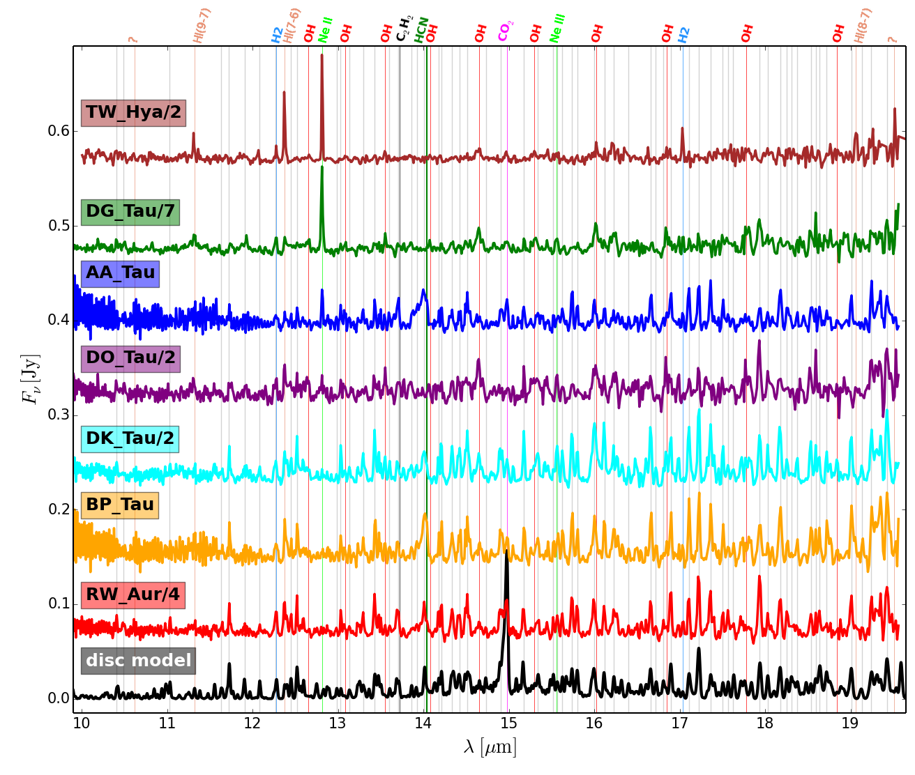
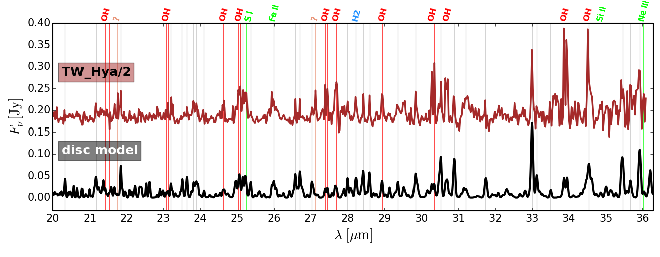
Figure 4: Upper plot: Seven continuum-subtracted $R\!=\!600$ Spitzer/IRS spectra of T Tauri stars (coloured lines) from Zhang et al. (2013, TW Hya) and Rigliaco et al. (2015, all other objects), arbitrarily shifted and scaled as indicated. At the bottom of the upper plot, the continuum-subtracted ProDiMo / FLiTs spectrum of our main disc model with $\rm gas/dust=1000$ is shown in black (convolved to $R=600$). Lower plot: The model spectrum is continued for longer wavelengths and compared to the observations of TW Hya with strong OH lines. The thin vertical coloured lines and top labels identify the molecules and ions. All unlabelled grey vertical lines indicate water lines. The salmon-coloured lines have no counterpart in the model; they are either high-excitation neutral hydrogen lines as indicated or are unidentified when labelled with “?”.

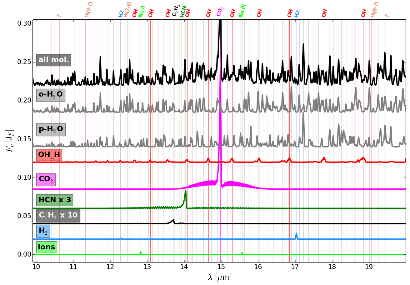
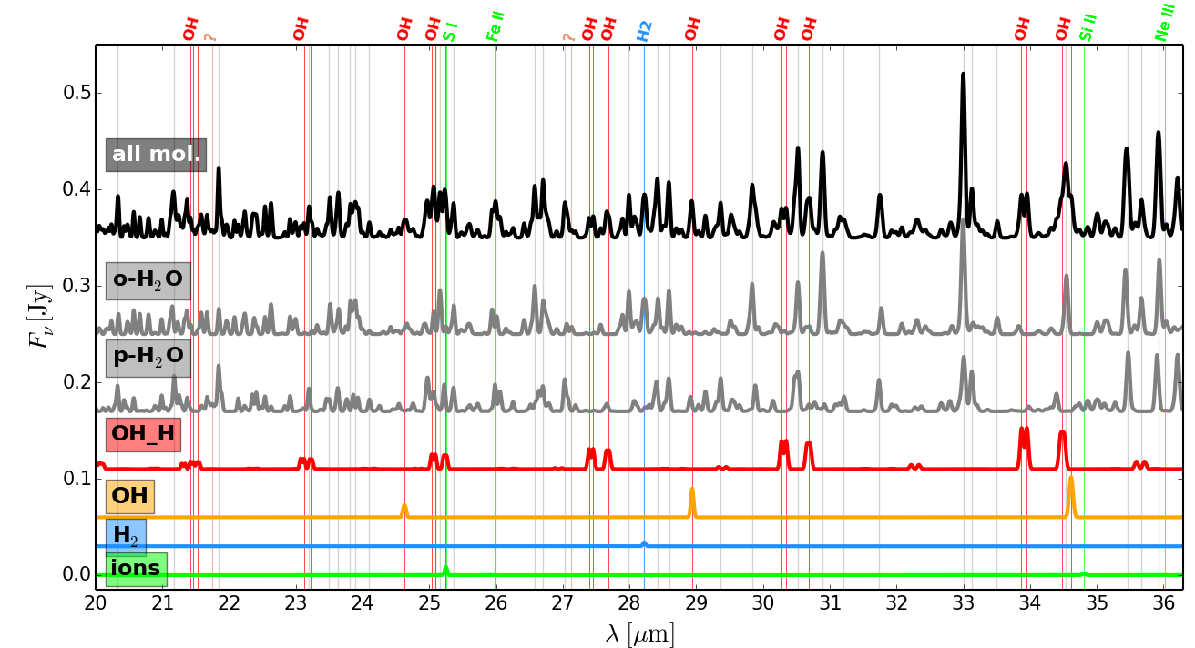
Figure 5: The $\rm g/d\!=\!1000$ model spectrum is decomposed into its main molecular constituents. We use the notation “OH_H” for ro-vibrational OH lines from the HITRAN database in contrast to the pure rotational lines computed in non-LTE and denoted by “OH”. These single molecule spectra are convolved to $R\!=\!600$ and arbitrarily shifted, but not scaled except for C₂H₂ and HCN. The C₂H₂ lines around 13.7 $\mu$m are very weak in the model, and are amplified by a factor of ten in this figure to make them visible. The vertical coloured lines and top labels identify the molecules and ions in the same way as in Fig. 4.

6 Results

6.1 Comparison to Spitzer observations

In Fig. 4, the FLiTs spectrum obtained from our standard ProDiMo disc model with gas/dust$\,=\,$1000 is compared to the continuum-subtracted Spitzer/IRS $R\!=\!600$ spectra of seven well-known T Tauri stars from Rigliaco et al. (2015) and Zhang et al. (2013). The figure shows numerous common emission features in model and observations. These emission features are often composed of several (up to hundreds of) overlapping individual lines, in particular at shorter wavelengths. Over 100 of such common spectral emission features (mostly water) have been identified and represented in Fig. 4 by coloured vertical thin lines, where the observational peaks have a corresponding counterpart in the model and vice versa. We were unable to find a corresponding match with the model for six observed lines/features. Three of these features are high excitation neutral hydrogen atomic lines as indicated in the figure, i.e. HI (9-7) 11.32 $\mu$m, HI (7-6) 12.37 $\mu$m, HI (8-7) 19.06 $\mu$m (Rigliaco et al., 2015), which are not included in our disc model, and three features remain unidentified at 10.62 $\mu$m, 21.75 $\mu$m, and 27.13 $\mu$m. We are not claiming, however, that our emission feature identifications are entirely accurate. Our molecular line data are possibly incomplete, and many of the spectral lines overlap at $R\!=\!600$ resolution; see Pontoppidan et al. (2010b) for more details.

The peak amplitudes are also in reasonable agreement with the observations, simultaneously for different molecules. Only our CO₂ emission feature at 15 $\mu$m is too strong by about a factor of 3. The different T Tauri stars show different overall levels and colours of line emission, and different emission feature fluxes for different molecules. With the exception of CO₂ 15 $\mu$m, the observed scatter in those feature fluxes is larger than the systematic deviations from the model.

6.2 Decomposed model spectrum

In Fig. 5 the model spectrum is decomposed into its molecular constituents, confirming the following results:

• Water is the main contributor to the mid-IR line spectra of T Tauri stars (Pontoppidan et al., 2010b).

• OH lines can be equally strong at longer wavelengths, clearly visible in the TW Hya spectrum (Najita et al., 2010; Zhang et al., 2013), and this is true for both the rotational OH and ro-vibrational OH_H lines.

• The CO₂ Q-branch of the $01^{1}0(1)\!\to\!00^{0}0(1)$ band at about 15 $\mu$m is regularly detected in T Tauri stars (Carr & Najita, 2008). The main model overpredicts the strength of this feature by about a factor of 3.

• The HCN Q-branch of the $01^{1}0\,\to\,00^{0}0$ band at 14 $\mu$m is detected in some T Tauri stars (Pascucci et al., 2009; Salyk et al., 2011; Najita et al., 2013), but not in all cases. Figure 5 shows that this feature is blended with one o-H₂O ($12_{7,6}\!\to\!11_{4,7}$) and one p-H₂O ($10_{7,3}\!\to\!9_{4,6}$) line. In our model the HCN Q-branch contribution to this feature is about 50%, which is possibly somewhat too weak in comparison to some T Tauri star observations.

• The C₂H₂ feature from the 000011u $\to$ 000000+g system at about 13.7 $\mu$m is detected in some T Tauri stars (Pascucci et al., 2009). It is very weak in the model, Fig. 5 shows it with magnification $\times 10$. This is likely to be a chemical effect as our disc model does not predict large concentrations of C₂H₂ in the relevant disc surface layers, although very abundant in deeper layers; see Sect. 6.5.

• Some T Tauri stars show strong [Ne II] 12.81 $\mu$m and [Ne III] 15.55 $\mu$m lines (Pascucci et al., 2007; Güdel et al., 2010) and some H₂ 17.03 $\mu$m and 28.22 $\mu$m emission, whereas others do not (Lahuis et al., 2007; Baldovin-Saavedra et al., 2011). In the model, we need particular phyical conditions to excite these lines, such as vertically extended low-density regions above the disc for the Ne lines. In the main model, these lines are rather weak ($1.3\times 10^{-18}\rm\,W/m^{2}$ and $6.6\times 10^{-19}\rm\,W/m^{2}$ for the main Ne II and Ne III lines), which agrees with many T Tauri observations (Aresu et al., 2012).

• The Fe II fine-structure line at $25.99\,\mu$m is strongly blended with a number of water lines. The line is actually very weak in the model $(3\times 10^{-20}\rm\,W/m^{2})$, as we are using a very low Fe element abundance in our model, assuming that Fe is locked in grains.

6.3 Role of dust/gas mass ratio and $T_{\rm gas}\!>\!T_{\rm dust}$

Figure 6 shows the total fluxes of all spectral lines emitted by the various molecules between 9.7 $\mu$m and 38 $\mu$m as a function of gas/dust ratio (g/d) in the model (at constant dust mass); see series of four models on the left side in Fig. 6. There is a very clear correlation for all molecules. As g/d increases, larger columns of gas are present above the $\tau_{\rm dust}\!=\!1$ surface, which leads to stronger emission lines. An alternative explanation can be provided by studying the heating/cooling balance. For larger g/d, more of the heating UV photons are absorbed by the gas, rather than by the dust, and this increase of gas heating is balanced by an increase of line cooling in the mid-IR spectral region. The measured dependencies of line fluxes versus g/d are about linear. A similar increase of all line fluxes can be produced in the model by changing some of the dust size and material properties such that the dust has lower UV and IR opacities.

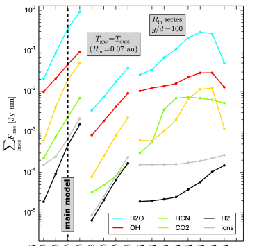
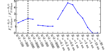
Figure 6: Upper part: Sum of all line fluxes emitted by the different molecules between 9.7 $\mu$m and 38 $\mu$m. The vertical dashed line indicates the main model as plotted in Figs. 4 and 5, which is broadly consistent with the observations. Lower part: Colour of the water line emission spectrum in the form of a ratio of two o-H₂O lines at about 12 $\mu$m and 27 $\mu$m. In the series of 4 models on the left, the gas/dust mass ratio in the disc is varied, the calculated gas temperatures are used, and $R_{\rm in}\!=\!0.07\,$au is assumed. In the series of 4 models in the centre, the gas/dust mass ratio in the disc is varied while $T_{\rm gas}\!=\!T_{\rm dust}$ and $R_{\rm in}\!=\!0.07\,$au are assumed. In the series of models on the right, the disc inner radius $R_{\rm in}$ is varied while assuming $\rm g/d\!=\!100$ and using the calculated gas temperatures. “H2O” is the combined emission from o-H₂O and p-H₂O, and “OH” is the combined emission from rotational OH lines and ro-vibrational OH_H lines; see Table 3.

The subsequent series of four models in Fig. 6 shows the results if we ignore the gas energy balance and artificially assume $T_{\rm gas}\!=\!T_{\rm dust}$. In this case, the line fluxes drop by about one order of magnitude with respect to a full model with the same g/d, underlining the importance of the gas over dust temperature contrast in the line emitting regions, as was already shown by Carmona et al. (2008) concerning H₂ lines and by Meijerink et al. (2009) concerning H₂O lines. As we show in Table 4, the overwhelming part of the observable molecular lines are optically thick and form on top of an optically thick dust continuum. For such lines, the Eddington-Barbier approximation

$$F_{\rm line}\propto S_{\nu}^{\rm line}(\tau_{\rm line}\!=\!1)-B_{\nu}\big{(}T_{\rm dust}(\tau_{\rm dust}\!=\!1)\big{)}$$ (3)

explains why the temperature contrast between gas and dust is so important. If we consider LTE, $S_{\nu}^{\rm line}(\tau_{\rm line}\!\!=\!\!1)=B_{\nu}\big{(}T_{\rm gas}(\tau_{\rm line}\!\!=\!\!1)\big{)}$ is valid. The weak line fluxes obtained from the $T_{\rm gas}\!=\!T_{\rm dust}$ approximation then result from the dust temperatures in the upper line-forming disc layers being slightly higher than the dust temperatures in the optically thick midplane. If that dust temperature slope were reversed (as expected in active discs powered by viscous heating), we would see absorption lines. In the full ProDiMo models, $T_{\rm gas}\!>\!T_{\rm dust}$ is a typical result (see Sect. 6.5) although this is not true for all layers and model parameters. The large amplification factor of about 10 finally results from the steepness of the Planck function at mid-IR wavelengths if the temperature drops below a few 100 K.

6.4 Dependence on inner disc radius

An increase of the gas/dust ratio from 100 to about 1000 provides an easy way to obtain mid-IR spectra that are broadly consistent with Spitzer/IRS line observations. However, it is unclear how robust this finding is, whether this physical interpretation is correct, or whether there are other ways to increase the emission line fluxes to the observed level. While looking for alternatives, we found that larger inner disc radii also imply higher mid-IR line fluxes in general; see also Antonellini et al. (2016). On the right side of Fig. 6, we show the results of a series of $\rm g/d\!=\!100$ models where the inner disc radius is systematically increased from its default value of $R_{\rm in}\!=\!0.07\,$au to values up to 30 au. All mid-IR line fluxes in the models are found to increase by factors of about 4 to 20 (depending on molecule), reach a maximum at a few au, and then decrease again. Figure 13 compares the line spectrum emergent from the main model to the line spectrum from the $\rm g/d\!=\!100$ model with $R_{\rm in}\!=\!3\,$au, showing that both options result in about the same overall line flux level. The main difference between these spectra is the overall colour of the line emission as shown in the lower part of Fig. 6 and discussed below. The line emission from the wall is bluer at maximum.

A similar behaviour was noticed for CO fundamental ro-vibrational lines and explained in (Woitke et al., 2016). As the inner disc radius $R_{\rm in}$ is increased in the model, the line emissions from the disc surface are more and more replaced by the direct emissions from the visible area of the inner rim of the disc; see Fig. 1. That wall is illuminated well by the star that heats the gas in the wall. Although we can only speculate about the physical structure of gas and dust in these walls, it seems reasonable to assume that very high gas densities are reached soon inside these walls; therefore the line emission takes place at unusually high densities where non-LTE effects are not likely to be important. As $R_{\rm in}$ increases, the size of the visible area of the wall increases with $R_{\rm in}^{2}$ and this effect is more important at first than the decrease of the wall temperature and line source functions in the wall. Once $R_{\rm in}$ reaches about 10 au, however, the wall becomes too cold and loses its ability to emit in the mid-IR, and so the line fluxes eventually diminish quickly.

The lower part of Fig. 6 shows the colour of the water emission spectrum in the form of the line flux ratio o-H₂O $\rm 13_{\,6,5}\to 12_{\,4,9}$ at 12.453 $\mu$m divided by o-H₂O $8_{5,4}\!\to\!8_{2,7}$ at $\lambda\!=\!27.059\,\mu$m (same lines as shown in Fig. 1). These two lines have excitation energies of 4213 K and 1806 K, respectively. Large line flux ratios correspond to a blue colour of the water emission line spectrum. We see that the models using the calculated $T_{\rm gas}$ are not only brighter but also bluer than the models assuming $T_{\rm gas}\!=\!T_{\rm dust}$. As $R_{\rm in}$ is increased in the model, the colour gets bluer first, as long as the wall emission continues to replace the disc surface emission, but then the colour becomes redder again as the temperature in the distant inner wall decreases. Interestingly, Banzatti et al. (2017) performed an observational study of water lines combined with inner disc radii obtained from high-resolution ro-vibrational CO lines, which show that the H₂O lines disappear from blue to red with increasing disc radius.

The lines of atomic ions and H₂ behave in different ways than the molecular lines discussed so far. The ion lines need an extended, tenuous, ionised, and hot layer high above the disc to become strong, whereas the excitation mechanism of the H₂ quadrupole lines is more complex (see Nomura & Millar, 2005; Nomura et al., 2007) and depends on wavelength. The H₂ lines at longer wavelengths form deep inside the disc in our models. Therefore, strong H₂ lines require large column densities and a sufficiently large temperature contrast $T_{\rm gas}\!>\!T_{\rm dust}$ well inside the disc, which is usually not present in our models.

More detailed investigations are required to study the spectroscopic differences between the line emission spectra obtained from disc walls and from disc surfaces; see Fig. 13. It seems possible that we can distinguish between disc surface and wall emission and that we can use the spectroscopically unresolved mid-IR spectroscopic fingerprints of wall emission to detect the presence of secondary irradiated disc walls with JWST at distances of a few au, for example caused by disc-planet interactions; see discussion in Sect. 7.2.

6.5 Chemical structure and line origin

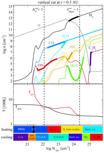
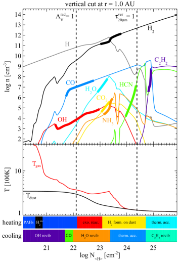
Figure 7: Abundances of mid-IR active molecules along vertical cuts through the disc at 0.3 au (left) and 1 au (right), plotted as a function of the vertical hydrogen nuclei column density $N_{\rm\langle H\rangle}$. The thick parts of the graphs highlight the mid-IR line forming regions of the respective molecules (see Eq. (4) and text). The two vertical dashed lines indicate where the radial dust optical depths is one ($A_{\rm V}^{\rm rad}=1$), and where the vertical dust optical depth at $\lambda=20\,\mu$m is one. The lower plot shows the vertical gas and dust temperature structure in the disc. The coloured bars below indicate the most important heating and cooling processes: rovib $=$ ro-vibrational, therm. acc. $=$ thermal accommodation, exo. reac. $=$ exothermal chemical reactions, form. $=$ formation.

Figure 7 shows two vertical cuts through the main model with $\rm g/d\!=\!1000$ at $r\!=\!0.3\,$au and $r\!=\!1\,$au, using the output from a $200\times 300$ model. The vertical structure is typical for photon dominated regions (PDRs; see e.g. Röllig et al., 2007), where the formation of molecules is suppressed by photodissociation at low column densities and triggered by subsequent UV dust absorption and molecular shielding. The resulting concentrations in discs over vertical $N_{\rm\langle H\rangle}$ can be compared, for example to (Najita et al., 2011). With respect to standard interstellar conditions, we find the following main differences in the planet-forming regions of protoplanetary discs:

• much higher densities,

• intense UV irradiation under acute angles,

• intense IR radiation emitted from the warm dust in the disc.

In particular, (2) implies that the classical $A_{V}$ scale does not fully represent the full 2D dust absorption and scattering effects for the UV penetration, which we use in our models. We chose to depict the vertical chemical and temperature structure as function of the vertical hydrogen nuclei column density $N_{\rm\langle H\rangle}$ and are highlighting the radial $A_{V}^{\rm rad}\!=\!1$ layer in Fig. 7, where the dust temperature starts to smoothly decline by an overall factor of about 3. The regions above the $A_{V}^{\rm rad}\!=\!1$ layer can be reached by stellar photons in a single flight, whereas the regions below are UV-illuminated mainly by photons scattered downward by the dust particles in the $A_{V}^{\rm rad}\!\approx\!1$ layers, with subsequent vertical dust absorption. Despite these differences, our vertical disc cuts resemble the following principal results of PDR modelling:

• molecular concentrations increase outside-in by many orders of magnitude before they typically reach some constant levels at relatively model-independent column densities,

• abundant molecules such as H₂ and CO form first because of their ability to self-shield,

• OH needs to form before H₂O can form,

• CO₂ forms in combination with H₂O,

• HCN and NH₃ form below H₂O and CO₂, and

• pure hydro-carbon molecules such as C₂H₂ are not abundant in the upper disc layers when the carbon to oxygen element ratio in the gas is $\rm C/O\!<\!1$.

The principal mechanisms that lead to such a sequence of increasing molecular complexity with depth in discs are described elsewhere (see e.g. Kamp & Dullemond, 2004; Nomura & Millar, 2005; Najita et al., 2011).

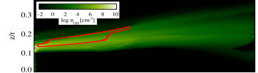
OH_H $\sf\lambda\!=\!20.1151\,\mu$m

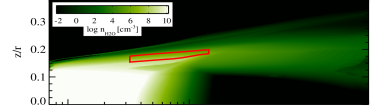
o-H2O  $\sf\lambda\!=\!23.8598\,\mu$m

CO2 $\sf\lambda\!=\!14.9777\,\mu$m

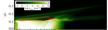
HCN $\sf\lambda\!=\!14.0264\,\mu$m

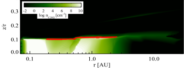
C2H2 $\sf\lambda\!=\!13.2039\,\mu$m

Figure 8: Molecular particle densities and mid-IR line origin. The six contour plots show, from top to bottom, the calculated particle densities of OH, H₂O, CO₂, HCN, NH₃, and C₂H₂ in the main model. For each molecule, we selected a strong line and encircled the disc regions with a red line that are responsible for 50% of the fluxes of those lines.

The thick sections of the abundance graphs in Fig. 7 highlight the line emitting regions, i.e. the layers that are found to be responsible for 70% of the observable line emissions from those molecules in that column. To evaluate these quantities, we use the escape probability method (Appendix A) to determine the emission region of each spectral line, and then average over all lines emitted in the mid-IR region of that molecule according to

$$\langle X\rangle=\sum\limits_{\rm lines}X\,F_{\rm line}\;\bigg{/}\;\sum\limits_{\rm lines}F_{\rm line}\ ,$$ (4)

where $X$ can be any quantity we are interested in; for example the vertical hydrogen column density at the upper or lower end of the line forming region. The values $F_{\rm line}$ are the integrated fluxes of all mid-IR emission lines of a particular molecule, where we have used all mid-IR emission lines listed in Table 3, and all ro-vibrational lines around $4.7\,\mu$m for CO. Table 4 shows additional emission line flux averaged properties of the molecules; for example the mean continuum and line optical depths or the gas and dust temperatures in the line forming regions, using Eq. (4).

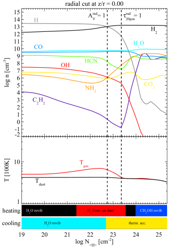
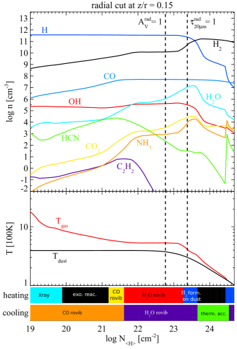
Figure 9: Abundances of mid-IR active molecules along radial cuts at constant $z/r$ through the disc model with inner disc radius $R_{\rm in}\!=\!1\,$au and $\rm g/d\!=\!100$, plotted as a function of the radial hydrogen nuclei column density $N_{\rm\langle H\rangle}$ (see text for how $N_{\rm\langle H\rangle}$ corresponds to $r$). The two vertical dashed lines indicate where the radial dust optical depth is one ($A_{\rm V}^{\rm rad}=1$), and where the radial dust optical depth at $\lambda=20\,\mu$m is one. The lower plot shows the gas and dust temperature along that cut. The coloured bars below indicate the most important heating and cooling processes.

The upper edges of the line forming layers shown in Fig. 7 usually coincide with a strong increase of molecular concentration, and the lower edges with the line ($+$ continuum) optical depth becoming huge. This highlights an important general finding of this work. The observable lines of different molecules probe the gas temperature in different layers of the disc, just where these molecules start to become abundant, along the following depth sequence:  OH (highest)  —  CO  —  H₂O and CO₂  —  HCN  —  C₂H₂ (deepest).  This is once more illustrated in Fig. 8, where we plot the 2D molecular concentrations and show how thin the line forming layers are for single ro-vibrational lines. Resolving these line formation regions spatially presents a numerical challenge to the model.

For additional orientation, in Fig. 7 we indicate the height at which the vertical dust optical depth at $\lambda\!=\!20\,\mu$m is one, $\tau^{\rm ver}_{\rm 20\,\mu m}\!=\!1$. The C₂H₂ abundance does eventually reach high values, but only below this height, so the C₂H₂ lines are covered by dust continuum in our model. Figures 7 and 8 show that the disc model has no water ice in the midplane at $r\!=\!0.3\,$au, whereas water ice is present at $r\!=\!1\,$au, as evident from the missing gaseous H₂O. This creates a local carbon-rich environment with gas element abundances $\rm C/O\!>\!1$, where C₂H₂ is about two orders of magnitude more abundant in the midplane than at $r\!=\!0.3$ au.

The lower part of Fig. 7 shows a few details about the gas energy balance in the inner disc regions. We generally find high gas temperatures of the order of several 1000 K in the diluted, photodissociated and partly ionised gas high above the disc. Once the first molecules form (in particular OH and CO), their ro-vibrational line cooling causes the gas temperature to drop to several 100 K, which leads to further molecule formation and accelerated cooling. This atomic $\to$ molecular transition hence occurs very suddenly and takes place well above the height $A_{V}^{\rm rad}\!=\!1$ at which the disc casts a shadow and the dust temperature starts to drop. At the $A_{V}^{\rm rad}\!=\!1$ height, small dust particles scatter the stellar UV photons partly downwards, which then penetrate deeper into the disc until the vertical dust optical depth reaches about $A_{V}^{\rm ver}\!\approx 3-5$. This effect generally leads to a positive temperature contrast between gas and dust of the order of a few 100 K in the layers responsible for most of the observable line emission.

There is an intermittent maximum of $T_{\rm gas}(z)$ as a function of column densities around $\log_{10}N_{\rm\langle H\rangle}\,{\rm[cm^{-2}]}\!\approx\!23.5$ in Fig. 7, which is caused by optical depth effects in the major cooling lines. At $A_{V}^{\rm rad}\!=\!1$ the line optical depths are still small and molecular line cooling works very efficiently. At slightly deeper layers, however, there is still some heating by UV photodissociation followed by exothermal reactions and H₂ re-formation on grain surfaces. But the line optical depths are already large here, making the cooling ineffective, and the temperature rises again. Eventually, the UV is completely absorbed and gas and dust temperatures equilibrate through inelastic collisions (thermal accommodation). Figure 7 also shows that a major part of the line forming region, from $A_{V}^{\rm rad}\!=\!1$ to $\tau_{\rm 20\,\mu m}^{\rm ver}\!=\!1$, is H rich. Thus, to discuss the non-LTE population of ro-vibrational states in discs, we need collision rates with atomic hydrogen.

In Fig. 9 we show two radial cuts (along constant $z/r$) through the model with inner radius $R_{\rm in}\!=\!1\,$au and $\rm g/d\!=\!100$. This time, the results are depicted as a function of radial  hydrogen nuclei density $N_{\rm\langle H\rangle}$ as measured from the inner wall. The gas densities are very high in this wall, $n_{\rm\langle H\rangle}\!\sim\!10^{13.5}\rm\,cm^{-3}$ at $z/r\!=\!0$ and $n_{\rm\langle H\rangle}\!\sim\!10^{11.5}\rm\,cm^{-3}$ at $z/r\!=\!0.15$. In order to resolve the line formation in these walls, we need a radial grid with initial increments of column densities or order $\sim\!10^{19}\rm\,cm^{-2}$. This requires radial inter-point distances as small as $\Delta r\sim\!10^{5}$ cm close to the wall, i.e. about 1 km or $10^{-8}$ au. The end of the line emitting regions ($\tau^{\rm rad}_{20\rm\,\mu m}\!=\!1$) is reached at about $N_{\rm\langle H\rangle}\!=\!10^{\,23.5}\rm\,cm^{-2}$ which, in the model with $R_{\rm in}\!=\!1\,$au, translates to $r\!=\!1.06\,$au at $z/r\!=\!0.15$ and $r\!=\!1.0006\,$au at $z/r\!=\!0$. Close to these walls, ProDiMo automatically switches to a PDR description where the molecular shielding factors, line escape, and pumping probabilities are measured in the radial direction.

These results show, however, that the walls are in fact not PDRs. At the high densities present in the wall, the two-body gas-phase chemical rates dominate over the UV-photon rates even if the wall is fully irradiated by the star, as in this model. Consequently, the molecular concentrations in Fig. 9 are already high on the left side, where the wall starts. The situation resembles the case of thermochemical equilibrium, where the UV, however, still plays a role in heating the gas. For very high densities, close to the midplane, we find radial layers in the wall where mid-IR lines of one particular molecule (such as H₂O) simultaneously provide the most important heating and cooling mechanism; that is the gas is in radiative equilibrium in consideration of the water line opacity, similar to for example brown dwarf atmospheres.

6.6 Impact of chemical rate networks and C/O ratio

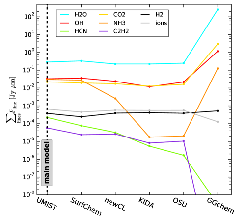
Figure 10: Total mid-IR molecular line emissions as a function of chemical rate network used in the model; see text for explanations.

The influence of the choice of the chemical rate network on the mid-IR line flux results is studied in Fig. 10. The base network used in this paper is UMIST 2012 (McElroy et al., 2013) with additional three-body (collider) reactions from UMIST 2006 (Woodall et al., 2007). All reactions among our selected species are taken into account from this database, completed by simple ice adsorption and desorption reactions, along with a few other special rates for excited hydrogen and PAHs; for details see (Kamp et al., 2017). The integrated mid-IR line fluxes of the molecules and ions in this UMIST model are again plotted on the left side of Fig. 10, denoted by “main model”. We then re-computed this model with different base chemical rate networks (using the gas temperature structure of the main model) as follows:

• SurfChem refers to a new warm surface chemical model (Thi et al. 2018 submitted).

• newCL is identical to the main UMIST model, but has one three-body reaction rate reduced, for $\rm\,N\,+\,H_{2}\,+\,M\,\longrightarrow\,NH_{2}\,+\,M$, from $10^{-26}\rm\,cm^{6}/s$ (Woodall et al., 2007) to $10^{-30}\rm\,cm^{6}/s$.

• KIDA 2014 (Kinetic Database for Astrochemistry, Wakelam et al., 2012, 2013).

• OSU 2009 (Ohio State University chemical network) from Eric Herbst.

• GGchem (Woitke et al., 2018) is a fast thermochemical equilibrium code that computes all molecular concentrations based on the principle to minimise the system Gibbs free energy.

We sorted the results according to the total HCN line flux, which shows a variation of about two orders of magnitude (not counting GGchem). Nitrogen is found to be predominantly atomic in the disc surface layers according to the KIDA and OSU models, and this is because these networks do not include the reaction  $\rm N\,+\,H_{2}\,+\,M\,\longrightarrow\,NH_{2}\,+\,M$. The newCL results demonstrate the importance of that reaction, which “activates” the nitrogen chemistry and eventually leads to the production of CN, HCN, and N₂ by follow-up neutral-neutral reactions. With reduced collider rate coefficient, the newCL results resemble the KIDA and OSU results more. Walsh et al. (2015) have also shown the necessity to include three-body reactions into their network to model the dense and warm chemistry in the planet-forming regions of protoplanetary discs.

The line fluxes based on the GGchem equilibrium chemistry model are extremely strong for water, CO₂, and OH. In thermochemical equilibrium, there are much more molecules present in the surface of the disc because photodissociation and other X-ray induced destruction mechanisms are not considered. However, since the gas is assumed to be oxygen rich, there are practically no HCN and C₂H₂ molecules in this model; therefore the emission features of those molecules are strongly suppressed. The bottom line is that none of the other chemical rate networks used in combination with our disc model bring us closer to the Spitzer/IRS line observations, which would require to increase the HCN and C₂H₂ lines fluxes while decreasing those of CO₂.

Another option is to consider an enrichment of the gas in the disc surface with carbon at au distances, see results plotted in Fig. 11. An increase of the carbon to oxygen ratio (C/O) $\to\!1$ actually shows the desired trend: the HCN lines become stronger while those of CO₂ get weaker. However, we do not consider this option to be a fully viable solution either. The water lines get too weak as C/O approaches unity, and when the C₂H₂ lines finally become observable, the HCN and NH₃ lines are already much too strong. However, it is noteworthy that a modest increase of C/O helps our model to get closer to the Spitzer observations. Najita et al. (2013) discussed the HCN/water ratio as a function of C/O, arriving at similar conclusions, and Pascucci et al. (2009, 2013) related these results to the Spitzer data.

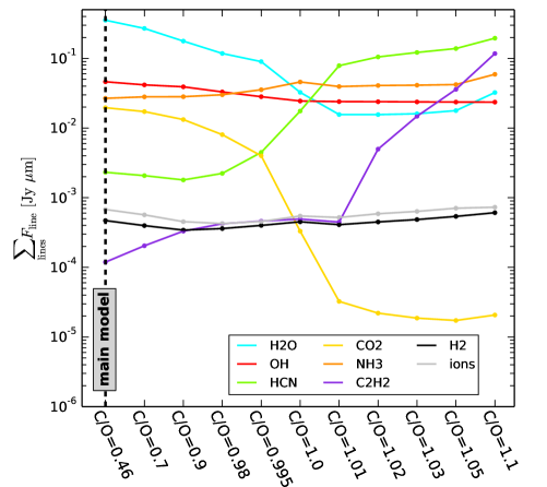
Figure 11: Total mid-IR molecular line emissions as a function of the carbon to oxygen ratio (C/O).

7 Summary and discussion

Previous analyses of the mid-IR molecular emission spectra of T Tauri stars have mostly been based on parameterised modelling approaches in which the temperatures and molecular concentrations are free parameters, which are then fitted to the observed line emission spectra. In the most simple case, single-point LTE slab models (Carr & Najita, 2011; Salyk et al., 2011) have been applied. More ambitious single-point non-LTE slab and simplified 2D disc models have been used by, for example Bruderer et al. (2015) and Bosman et al. (2017), focussing on HCN and CO₂, respectively. In an attempt to eliminate the current uncertainties in chemical rate networks and heating/cooling physics in discs, the scientific procedure in these works can be summarised as follows: (i) derive temperatures and molecular column densities from the line observations, (ii) divide the column densities by each other to determine the molecular abundance ratios, and (iii) adjust element abundances and chemical rate parameters in the models until agreement is achieved.

In this paper, we have followed a very different strategy. We used the full 2D chemical and temperature results from complex thermochemical disc models. Without any detailed fitting, we showed that our model spectra are broadly consistent with the observed properties of Spitzer/IRS line emission spectra when we either assume large gas/dust ratios or when we consider discs with directly irradiated vertical walls at au distances. A number of averaged molecular properties from our models are listed in Table 4 for completeness.

We think that both modelling strategies are valid approaches, however, we would like to highlight a few general results from our modelling approach that we think are robust:

• The mid-IR molecular lines from protoplanetary discs are optically thick and form above an optically thick dust continuum, therefore the temperature contrast between gas and dust has a decisive influence on the resulting line fluxes.

• In PDR modelling, as for example performed in this paper, the molecular concentrations usually increase by many orders of magnitude with increasing depth. As both density and concentration increase outside-in in discs, the mid-IR molecular line optical depths will reach unity in some layer. Most of the observed line photons from that molecule originate from this layer. Subsequently, the line optical depths become huge and/or the continuum optical depths exceed unity. In both cases, the line flux contributions of the molecules situated in those deeper layers is small.

• Consequently, the mid-IR lines of different molecules form in rather thin shells at different geometrical depths, where the physical conditions can be very different. We find the molecular lines in our models to be emitted from a succession of onion-like shells as sketched in Fig. 12, first OH, then CO, then H₂O etc., which we consider as a natural and straightforward result of the applied PDR physics.

• Molecular column densities derived from observations can only provide averaged information about the concentration of the molecules above the $\tau_{\rm dust}\!=\!1$ disc surface, and these values physically depend on the dust opacities assumed. Therefore, a realistic treatment of the dust continuum is an important ingredient for any mid-IR line modelling.

• Different lines of different molecules are emitted from different radial disc zones. Therefore, dividing column densities derived from observations by each other can produce misleading mixing ratios.

• Studying molecular emission lines from the tenuous disc surface alone might be incomplete as the molecular lines are also partly emitted from the inner rim where the line excitation and chemical conditions are different.

7.1 LTE or non-LTE ?

Bruderer et al. (2015) and Bosman et al. (2017) have presented detailed investigations of non-LTE effects in discs, including the pumping of the ro-vibrational states by IR dust emission, concerning HCN and CO₂, respectively. Their conclusion is that non-LTE effects are important for both flux and line shape, in particular with regard to IR molecular bands at shorter wavelengths (3 $\mu$m and 4.5 $\mu$m for HCN and CO₂, respectively). Thi et al. (2013) presented a thorough discussion of non-LTE effects on fundamental CO emission from discs at similar wavelengths.

In contrast to these results, Meijerink et al. (2009), using parameterised chemical concentrations, and Antonellini et al. (2015, 2016), using full thermochemical models, found no dramatic non-LTE effects for the water emission. Our results show no significant deviations of the water line fluxes either, if we force the water molecules to be populated in LTE. Concerning CO₂ and HCN, our models currently do not allow for a non-LTE treatment. However, the ro-vibrational OH lines in our model, which are treated in LTE, blend in nicely with the pure rotational OH lines, which are treated in non-LTE. This agrees well with the TW Hya observations (Fig. 4).

We interpret this dispute about the importance of non-LTE effects as follows. Our models suggest that the concentrations of most molecules are vanishingly small in the upper disc layers and only become suddenly abundant at rather deep layers, where gas densities are already as large as $10^{12}\rm\,cm^{-3}$; see Figs. 7. Under such conditions, non-LTE effects are expected to be small. In contrast, when assuming constant concentrations in the entire column as in (Meijerink et al., 2009), (Bruderer et al., 2015) and (Bosman et al., 2017), the lines are expected to form at higher altitudes, i.e. in a tenuous environment where non-LTE effects can be important. If the molecular lines are directly emitted from vertical disc walls, wherein the densities are even higher, non-LTE effects are expected to be even less significant.

However, more detailed investigations are required here. The ro-vibrational lines of the OH radical are a particularly interesting case because OH already forms at high altitudes where non-LTE effects are likely to be important.

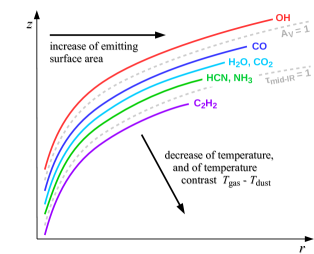
Figure 12: Onion-like shells of mid-IR line forming regions probing the disc temperature at different depths.

Table 4: Mean molecular properties in the main disc model with $\rm gas/dust\!=\!1000$, in consideration of two vertical cuts; cf. Fig. 7.

​​molecule​​	​​vertical cut​​	$\langle\lambda\rangle\rm\,[\mu m]^{(1)}$	col. density $[\rm cm^{-2}]^{(2)}$	$\langle$line formation$\rangle\,[\rm cm^{-2}]^{(1,3)}$	$\langle\tau_{\rm line}\rangle^{(1,2)}$	$\langle\tau_{\rm dust}\rangle^{(1,2)}$	$\langle T_{\rm gas}\rangle\rm\,[K]^{(1,3)}$​​​​
OH	$r\!=\!0.3$ au	24.8	$1.5(+17)$	$4(+14)-2(+16)$	36	790	1180
CO	$r\!=\!0.3$ au	4.71	$1.3(+23)$	$1(+18)-4(+19)$	$1.1(+7)$	1100	470
CO2	$r\!=\!0.3$ au	14.9	$1.4(+21)$	$6(+15)-8(+16)$	$4.6(+5)$	840	480
H2O	$r\!=\!0.3$ au	18.7	$1.3(+23)$	$8(+17)-3(+19)$	$1.4(+6)$	840	480
NH3	$r\!=\!0.3$ au	11.3	$2.2(+22)$	$6(+15)-1(+17)$	$2.8(+6)$	970	460
H2	$r\!=\!0.3$ au	15.9	$5.0(+26)$	$4(+22)-8(+23)$	810	840	360
HCN	$r\!=\!0.3$ au	14.0	$5.2(+21)$	$9(+13)-1(+16)$	$1.9(+6)$	860	330
C2H2	$r\!=\!0.3$ au	13.8	$8.2(+19)$	$3(+14)-1(+17)$	$1.8(+4)$	860	230
OH	$r\!=\!1$ au	24.3	$5.9(+16)$	$2(+14)-1(+16)$	12	230	720
CO	$r\!=\!1$ au	4.69	$9.9(+20)$	$2(+16)-7(+18)$	$1.8(+5)$	340	360
CO2	$r\!=\!1$ au	15.0	$8.8(+16)$	$3(+15)-2(+16)$	31	250	330
H2O	$r\!=\!1$ au	22.2	$1.4(+19)$	$2(+17)-4(+18)$	$1.2(+3)$	250	320
NH3	$r\!=\!1$ au	11.1	$4.4(+17)$	$3(+15)-3(+16)$	90	300	320
H2	$r\!=\!1$ au	17.1	$1.5(+26)$	$2(+22)-2(+23)$	330	250	280
HCN	$r\!=\!1$ au	14.1	$6.1(+20)$	$5(+14)-3(+17)$	$3.2(+5)$	260	140
C2H2	$r\!=\!1$ au	13.8	$1.2(+21)$	$5(+16)-7(+18)$	$6.4(+5)$	260	130

⁽¹⁾: Mean properties denoted by $\langle\cdot\rangle$ are calculated according to Eq. (4) as average over all included mid-IR emission lines listed in Table 3, weighted by line flux,  ⁽²⁾: Maximum values reached in the midplane,  ⁽³⁾: Values in the line forming regions.

7.2 Surface or wall emission?

Detecting disc gaps at au scales associated with planet formation is a difficult task, even with the currently best observational techniques such as IR interferometry or ALMA (ALMA Partnership et al., 2015; Pinte et al., 2016). The information obtained from continuum data is necessarily limited to the dust component, but does not reveal the structure of the gas.

As this paper demonstrates, mid-IR molecular emission lines are partly emitted from the disc surface and partly emitted from irradiated disc walls (Fig. 1). We have only discussed truncated discs with fully irradiated walls in this paper and further modelling of discs with gaps is certainly required. But we can say with confidence already that there are significant spectroscopic differences (strength, colour, and ratios of the emission features of different molecules) between disc surface emission and disc wall emission (see Fig. 13). These differences are caused by the different temperature, density, and radiation field conditions in the disc surfaces compared to those in the walls. Therefore, high S/N observations of spectroscopically unresolved mid-IR molecular emission spectra, as will become possible with JWST, might offer an alternative way to detect and characterise disc walls at au distances in T Tauri stars.

Considering discs with gaps, only a small fraction of the vertical walls at the outer end of a gap might be fully irradiated, or these walls might be completely submerged in the shadow of a tall inner disc, in which case the implied changes of the mid-IR line spectrum are expected to be small. But if there are directly irradiated parts of a disc wall present at au scales, it might be possible to detect these with JWST based on the spectroscopic fingerprints of molecular wall emission. Our models are well suited for subsequent research on this matter as the models cover all relevant physics and chemistry.

8 Conclusions and outlook

We have used full 2D thermochemical disc models to calculate complete atomic and molecular emission spectra from T Tauri stars between $9.7\,\mu$m and $38\,\mu$m, using a mixture of LTE and non-LTE techniques. We introduced FLiTs to ray trace tens of thousands of mid-IR molecular emission lines in one shot.

Without detailed fitting of disc shape or dust opacities, we find a reasonable agreement with previously published Spitzer/IRS spectra. To achieve this agreement, however, we need to increase the gas/dust ratio from 100 to about 1000 at radial distances of a few au, or consider transitional discs which have distant inner walls at a few au or illuminated secondary walls following gaps as expected for planet-disc interactions.

Generally speaking, strong mid-IR lines are emitted from exposed, irradiated molecules. In our models, such molecules exist when (i) the gas/dust ratio is large; (ii) the dust is unusually transparent in the UV, for example when all small grains are removed; or when (iii) dust settling is very strong. Concerning the third option, the sub-micron grains (the main UV opacity carriers) would need to be removed from the disc surface by gravitational settling at au distances. According to the physical description of dust settling used in this paper (Dubrulle et al., 1995, applying the midplane gas density), we find it difficult to explain the bright mid-IR line emission from T Tauri stars by settling. Antonellini et al. (2015, 2016) arrived at similar conclusions. However, Riols & Lesur (2018) have proposed an improved treatment of settling, taking into account the decrease of gas density with height, which fits their numerical mixing experiments. According to Riols & Lesur’s settling description, it seems indeed possible to remove the sub-micron grains from the disc surface by gravitational settling. More numerical experiments are required to verify this solution.

Another possibility is to have (iv) molecules situated in dense illuminated vertical disc walls, where the two-body gas phase reaction rates are huge and can compensate the losses by UV dissociation. The resulting molecular concentrations are rather independent of the UV irradiation, and thus favour the existence of irradiated molecules.

In all these scenarios, large radiation fields overlap with large molecular concentrations, and the heating UV photons are absorbed by the molecules rather then by the dust. More detailed investigations are required to study to what extent we can disentangle wall emission from disc surface emission, and to possibly use new JWST line observations to detect discs with illuminated secondary walls at au scales. Taking into account complementary spectral energy distribution and continuum IR visibility data should allow us to reject some of these scenarios.

Future non-LTE investigations require collision rates with atomic hydrogen because the line forming regions are partly H rich and H₂ poor, as is true for CO (Thi et al., 2013). Ro-vibrational lines of the OH radical are expected to show the strongest non-LTE effects because these lines form at high altitudes above the disc.

In all our models that broadly agree with the observed mid-IR line strengths, the mid-IR lines of H₂O, OH, CO₂, HCN, and C₂H₂ are optically thick. Therefore, we conclude that mid-IR line fluxes are not good tracers of column densities. Instead, we find that the gas/dust temperature contrast has a decisive influence on the strength and shape of the IR molecular emission spectra. We see no direct influence of the ice lines on the emitted IR spectra, as ice formation takes place only very deep in the disc midplane ($A_{V}\!\ga\!10$). However, vertical mixing processes could establish a link to the ice lines.

The chemistry in the planet-forming and IR line emitting regions of protoplanetary discs needs further attention, including three-body reactions, warm surface chemistry, and combustion. At the moment, models with different chemical rate networks predict rather different mid-IR spectra, and our standard chemical rate network seems to somewhat overpredict CO₂, and underpredict HCN and C₂H₂. These molecular concentrations are strongly affected by the assumed C/O ratio in the gas. For $\rm C/O\!\to\!1$, we would expect more HCN, more C₂H₂, and less CO₂ to form, which could help to better understand the smultaneous emissions from all these molecules other than water. If oxygen is consumed in deeper layers to form water ice, there is a cold trap for oxygen in the midplane, and if some turbulent mixing establishes a physical link from the spectroscopically active surface layers to that cold trap, the oxygen abundance would actually be expected to decrease over time.

Acknowledgements:  We thank the anonymous referee for the insightful remarks that helped improve the paper. The research leading to these results has received funding from the European Union Seventh Framework Programme FP7-2011 under grant agreement no 284405. The computer simulations were carried out on the UK MHD Consortium parallel computer at the University of St Andrews, funded jointly by STFC and SRIF.

Appendix A Escape probability model

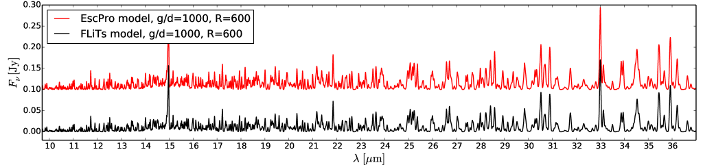
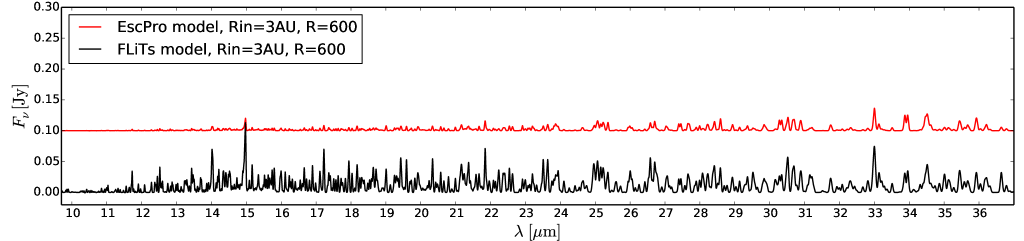
Figure 13: Comparison between continuum-subtracted FLiTs spectra (black), ray traced for disc inclination $45^{\circ}$, and spectra directly obtained from our vertical escape probability method (red, “EscPro”), both convolved to $R\!=\!600$ spectral resolution. The agreement is remarkable for the main model with gas/dust ratio $\rm g/d\!=\!1000$ and inner disc radius $R_{\rm in}\!=\!0.07\,$au (upper plot), where disc surface emission dominates. However, for the truncated disc model with $\rm g/d\!=\!100$ and $R_{\rm in}\!=\!3\,$au (lower plot), the escape probability method fails because the line photons are mostly emitted sideways through the inner disc wall, in which case the EscPro spectrum results to be too faint, and too red.

The details of our simplified non-LTE treatment of atomic and molecular level populations (escape probability method) are explained in (Woitke et al., 2009, Sect. 6.1 therein). This article provides the general concept, physical quantities and symbols used. Once the model is completed, we can calculate the vertically escaping line luminosity [erg/s] of transition $u\!\to\!l$ as

$$L_{\rm line}=\sum\limits_{\rm cells}n_{u}V_{\rm cell}\;h\nu_{ul}\;A_{ul}\;P_{ul}^{\rm pump}\!(\tau_{ul}^{\rm ver})\;\exp(-\tau^{\rm ver}_{\rm dust})\ ,$$ (5)

where $n_{u}$ [cm^-3] is the upper level population, $V_{\rm cell}$ [cm³] the volume of a computational cell, $\nu_{ul}$ the line centre frequency, and $A_{ul}$ [s^-1] the Einstein emission coefficient. For the escape probability, we take the probability of line photons to reach the disc surface on a vertically upward pointed ray; see $P_{ul}^{\rm pump}$ in Eq. (83) of (Woitke et al., 2009). Vertical line centre and continuum optical depths are given by

$$\tau_{ul}^{\rm ver} = \frac{A_{ul}c^{3}}{8\pi\nu_{ul}^{3}}\int_{z}^{\infty}\frac{1}{\Delta\nu_{\rm D}}\left(n_{l}\frac{g_{u}}{g_{l}}-n_{u}\right)\;dz^{\prime}$$ (6)

$$\tau^{\rm ver}_{\rm dust} = \int_{z}^{\infty}\kappa^{\rm ext}_{\nu_{ul}}\;dz^{\prime}\ ,$$ (7)

where $\Delta\nu_{\rm D}$ is the (thermal$\,+\,$turbulent) Doppler width of the line. To calculate Eq. (7) we use a simple Simpson integration based on the given dust particle densities and opacities. Concerning Eq. (6), we perform an implicit integration by assuming that $n_{u}/n_{l}$ is constant in each cell and that the line optical depth used to calculate the population numbers refer to the bottom of each cell. In order to account for the lower half of the disc, the disc is mirrored at the midplane and the optical depths are computed across the disc to the other surface, such that each computational cell actually occurs twice in Eq. (5). Finally, the line luminosity is converted into line flux at distance $d$ as

$$F_{\rm line}=\frac{1}{4\pi\,d^{2}}\,L_{\rm line}\ .$$ (8)

Equation 5 provides an easy way to identify the cells (or spatial disc region) that are most important for the emission of a given spectral line. We have used this concept to highlight the line emission layers and regions in Figs. 7, 8, and Table 4.

Figure 13 shows that the agreement with the full ray-tracing FLiTs spectrum is excellent for the main model, whereas we cannot apply the escape probability method to discs with au-sized inner holes, where the lines are mostly emitted by the inner disc wall. To summarise,

• The escape probability spectra often provide very good first guesses of the line emission spectra and come for free with ProDiMo, i.e. they do not need any additional computational time to be calculated.

• The escape probability technique always predicts line emission. This is physically not guaranteed. Infrared line absorption is expected for large disc inclinations and for active discs that are heated internally by accretion, where the vertical temperature gradients are reversed.

• The escape probability spectra do not contain any line profile information, but are useful only for spectral resolutions up to a couple of 1000.

• The escape probability technique cannot be applied to transitional discs with inner disc radii larger than a few $1/10^{\rm th}$ of au, as the line photons in such discs rather escape sideways through the inner disc wall.

References

- Agúndez et al. (2008) Agúndez, M., Cernicharo, J., & Goicoechea, J. R. 2008, A&A, 483, 831
- ALMA Partnership et al. (2015) ALMA Partnership, Brogan, C. L., Pérez, L. M., et al. 2015, ApJ, 808, L3
- Antonellini et al. (2016) Antonellini, S., Kamp, I., Lahuis, F., et al. 2016, A&A, 585, A61
- Antonellini et al. (2015) Antonellini, S., Kamp, I., Riviere-Marichalar, P., et al. 2015, A&A, 582, A105
- Aresu et al. (2012) Aresu, G., Meijerink, R., Kamp, I., et al. 2012, A&A, 547, A69
- Avramenko & Krasnenkov (1966) Avramenko, L. I. & Krasnenkov, V. M. 1966, Bull. Acad. Sci. USSR Div. Chem. Sci. (Engl. Transl.), 15, 394
- Baldovin-Saavedra et al. (2012) Baldovin-Saavedra, C., Audard, M., Carmona, A., et al. 2012, A&A, 543, A30
- Baldovin-Saavedra et al. (2011) Baldovin-Saavedra, C., Audard, M., Güdel, M., et al. 2011, A&A, 528, A22
- Banzatti et al. (2014) Banzatti, A., Meyer, M. R., Manara, C. F., Pontoppidan, K. M., & Testi, L. 2014, ApJ, 780, 26
- Banzatti et al. (2017) Banzatti, A., Pontoppidan, K. M., Salyk, C., et al. 2017, ApJ, 834, 152
- Birnstiel et al. (2012) Birnstiel, T., Klahr, H., & Ercolano, B. 2012, A&A, 539, A148
- Blake & Boogert (2004) Blake, G. A. & Boogert, A. C. A. 2004, ApJ, 606, L73
- Bosman et al. (2017) Bosman, A. D., Bruderer, S., & van Dishoeck, E. F. 2017, A&A, 601, A36
- Brittain et al. (2009) Brittain, S. D., Najita, J. R., & Carr, J. S. 2009, ApJ, 702, 85
- Bruderer et al. (2015) Bruderer, S., Harsono, D., & van Dishoeck, E. F. 2015, A&A, 575, A94
- Carmona et al. (2014) Carmona, A., Pinte, C., Thi, W. F., et al. 2014, A&A, 567, A51
- Carmona et al. (2017) Carmona, A., Thi, W. F., Kamp, I., et al. 2017, A&A, 598, A118
- Carmona et al. (2008) Carmona, A., van den Ancker, M. E., Henning, T., et al. 2008, A&A, 477, 839
- Carr & Najita (2008) Carr, J. S. & Najita, J. R. 2008, Science, 319, 1504
- Carr & Najita (2011) Carr, J. S. & Najita, J. R. 2011, ApJ, 733, 102
- Daniel et al. (2011) Daniel, F., Dubernet, M.-L., & Grosjean, A. 2011, A&A, 536, A76
- Dere et al. (1997) Dere, K. P., Landi, E., Mason, H. E., Monsignori Fossi, B. C., & Young, P. R. 1997, A&AS, 125, 149
- Du et al. (2015) Du, F., Bergin, E. A., & Hogerheijde, M. R. 2015, ApJ, 807, L32
- Dubrulle et al. (1995) Dubrulle, B., Morfill, G., & Sterzik, M. 1995, Icarus, 114, 237
- Faure & Josselin (2008) Faure, A. & Josselin, E. 2008, A&A, 492, 257
- Fedele et al. (2013) Fedele, D., Bruderer, S., van Dishoeck, E. F., et al. 2013, A&A, 559, A77
- Fedele et al. (2011) Fedele, D., Pascucci, I., Brittain, S., et al. 2011, ApJ, 732, 106
- Folsom et al. (2012) Folsom, C. P., Bagnulo, S., Wade, G. A., et al. 2012, MNRAS, 422, 2072
- Galvao & Poveda (2015) Galvao, B. R. L. & Poveda, L. A. 2015, The Journal of Chemical Physics, 142, 184302
- Güdel et al. (2010) Güdel, M., Lahuis, F., Briggs, K. R., et al. 2010, A&A, 519, A113
- Hein Bertelsen et al. (2014) Hein Bertelsen, R. P., Kamp, I., Goto, M., et al. 2014, A&A, 561, A102
- Hein Bertelsen et al. (2016a) Hein Bertelsen, R. P., Kamp, I., van der Plas, G., et al. 2016a, A&A, 590, A98
- Hein Bertelsen et al. (2016b) Hein Bertelsen, R. P., Kamp, I., van der Plas, G., et al. 2016b, MNRAS, 458, 1466
- Herczeg et al. (2007) Herczeg, G. J., Najita, J. R., Hillenbrand, L. A., & Pascucci, I. 2007, ApJ, 670, 509
- Ilee et al. (2014) Ilee, J. D., Fairlamb, J., Oudmaijer, R. D., et al. 2014, MNRAS, 445, 3723
- Ilee et al. (2013) Ilee, J. D., Wheelwright, H. E., Oudmaijer, R. D., et al. 2013, MNRAS, 429, 2960
- Kama et al. (2016) Kama, M., Bruderer, S., Carney, M., et al. 2016, A&A, 588, A108
- Kama et al. (2015) Kama, M., Folsom, C. P., & Pinilla, P. 2015, A&A, 582, L10
- Kamp & Dullemond (2004) Kamp, I. & Dullemond, C. P. 2004, ApJ, 615, 991
- Kamp et al. (2017) Kamp, I., Thi, W.-F., Woitke, P., et al. 2017, A&A, 607, A41
- Kamp et al. (2010) Kamp, I., Tilling, I., Woitke, P., Thi, W., & Hogerheijde, M. 2010, A&A, 510, A18+
- Lahuis et al. (2007) Lahuis, F., van Dishoeck, E. F., Blake, G. A., et al. 2007, ApJ, 665, 492
- Lahuis et al. (2006) Lahuis, F., van Dishoeck, E. F., Boogert, A. C. A., et al. 2006, ApJ, 636, L145
- Lique (2015) Lique, F. 2015, MNRAS, 453, 810
- McElroy et al. (2013) McElroy, D., Walsh, C., Markwick, A. J., et al. 2013, A&A, 550, A36
- Meijerink et al. (2009) Meijerink, R., Pontoppidan, K. M., Blake, G. A., Poelman, D. R., & Dullemond, C. P. 2009, ApJ, 704, 1471
- Min et al. (2016) Min, M., Bouwman, J., Dominik, C., et al. 2016, A&A, 593, A11
- Min et al. (2009) Min, M., Dullemond, C. P., Dominik, C., de Koter, A., & Hovenier, J. W. 2009, A&A, 497, 155
- Najita et al. (2011) Najita, J. R., Ádámkovics, M., & Glassgold, A. E. 2011, ApJ, 743, 147
- Najita et al. (2013) Najita, J. R., Carr, J. S., Pontoppidan, K. M., et al. 2013, ApJ, 766, 134
- Najita et al. (2010) Najita, J. R., Carr, J. S., Strom, S. E., et al. 2010, ApJ, 712, 274
- Nomura et al. (2007) Nomura, H., Aikawa, Y., Tsujimoto, M., Nakagawa, Y., & Millar, T. J. 2007, ApJ, 661, 334
- Nomura & Millar (2005) Nomura, H. & Millar, T. J. 2005, A&A, 438, 923
- Offer et al. (1994) Offer, A. R., van Hemert, M. C., & van Dishoeck, E. F. 1994, J. Chem. Phys., 100, 362
- Pascucci et al. (2009) Pascucci, I., Apai, D., Luhman, K., et al. 2009, ApJ, 696, 143
- Pascucci et al. (2013) Pascucci, I., Herczeg, G., Carr, J. S., & Bruderer, S. 2013, ApJ, 779, 178
- Pascucci et al. (2007) Pascucci, I., Hollenbach, D., Najita, J., et al. 2007, ApJ, 663, 383
- Pascucci & Sterzik (2009) Pascucci, I. & Sterzik, M. 2009, ApJ, 702, 724
- Pascucci et al. (2011) Pascucci, I., Sterzik, M., Alexander, R. D., et al. 2011, ApJ, 736, 13
- Pinte et al. (2016) Pinte, C., Dent, W. R. F., Ménard, F., et al. 2016, ApJ, 816, 25
- Pinte et al. (2006) Pinte, C., Ménard, F., Duchêne, G., & Bastien, P. 2006, A&A, 459, 797
- Pinte et al. (2018) Pinte, C., Ménard, F., Duchêne, G., et al. 2018, A&A, 609, A47
- Pontoppidan et al. (2009) Pontoppidan, K. M., Meijerink, R., Dullemond, C. P., & Blake, G. A. 2009, ApJ, 704, 1482
- Pontoppidan et al. (2010a) Pontoppidan, K. M., Salyk, C., Blake, G. A., & Käufl, H. U. 2010a, ApJ, 722, L173
- Pontoppidan et al. (2010b) Pontoppidan, K. M., Salyk, C., Blake, G. A., et al. 2010b, ApJ, 720, 887
- Rigliaco et al. (2015) Rigliaco, E., Pascucci, I., Duchene, G., et al. 2015, ApJ, 801, 31
- Riols & Lesur (2018) Riols, A. & Lesur, G. 2018, ArXiv e-prints [arXiv:1805.00458]
- Röllig et al. (2007) Röllig, M., Abel, N. P., Bell, T., et al. 2007, A&A, 467, 187
- Rothman et al. (2013) Rothman, L. S., Gordon, I. E., Babikov, Y., et al. 2013, J. Quant. Spec. Radiat. Transf., 130, 4
- Rothman et al. (1998) Rothman, L. S., Rinsland, C. P., Goldman, A., et al. 1998, J. Quant. Spec. Radiat. Transf., 60, 665
- Sacco et al. (2012) Sacco, G. G., Flaccomio, E., Pascucci, I., et al. 2012, ApJ, 747, 142
- Salyk et al. (2015) Salyk, C., Lacy, J. H., Richter, M. J., et al. 2015, ApJ, 810, L24
- Salyk et al. (2008) Salyk, C., Pontoppidan, K. M., Blake, G. A., et al. 2008, ApJ, 676, L49
- Salyk et al. (2011) Salyk, C., Pontoppidan, K. M., Blake, G. A., Najita, J. R., & Carr, J. S. 2011, ApJ, 731, 130
- Schöier et al. (2005) Schöier, F. L., van der Tak, F. F. S., van Dishoeck, E. F., & Black, J. H. 2005, A&A, 432, 369
- Semenov & Wiebe (2011) Semenov, D. & Wiebe, D. 2011, ApJS, 196, 25
- Tazaki & Nomura (2015) Tazaki, R. & Nomura, H. 2015, ApJ, 799, 119
- Thi & Bik (2005) Thi, W.-F. & Bik, A. 2005, A&A, 438, 557
- Thi et al. (2013) Thi, W. F., Kamp, I., Woitke, P., et al. 2013, A&A, 551, A49
- Thi et al. (2005) Thi, W.-F., van Dalen, B., Bik, A., & Waters, L. B. F. M. 2005, A&A, 430, L61
- Thi et al. (2011) Thi, W.-F., Woitke, P., & Kamp, I. 2011, MNRAS, 412, 711
- van der Tak et al. (2007) van der Tak, F. F. S., Black, J. H., Schöier, F. L., Jansen, D. J., & van Dishoeck, E. F. 2007, A&A, 468, 627
- Wakelam et al. (2012) Wakelam, V., Herbst, E., Loison, J.-C., et al. 2012, ApJS, 199, 21
- Wakelam et al. (2013) Wakelam, V., Smith, I. W. M., Loison, J.-C., et al. 2013, ArXiv e-prints [arXiv:1310.4350]
- Walsh et al. (2015) Walsh, C., Nomura, H., & van Dishoeck, E. 2015, A&A, 582, A88
- Woitke et al. (2018) Woitke, P., Helling, C., Hunter, G. H., et al. 2018, A&A, 614, A1
- Woitke et al. (2009) Woitke, P., Kamp, I., & Thi, W.-F. 2009, A&A, 501, 383
- Woitke et al. (2016) Woitke, P., Min, M., Pinte, C., et al. 2016, A&A, 586, A103
- Woitke et al. (2011) Woitke, P., Riaz, B., Duchêne, G., et al. 2011, A&A, 534, A44
- Woodall et al. (2007) Woodall, J., Agúndez, M., Markwick-Kemper, A. J., & Millar, T. J. 2007, A&A, 466, 1197
- Wrathmall et al. (2007) Wrathmall, S. A., Gusdorf, A., & Flower, D. R. 2007, MNRAS, 382, 133
- Zhang et al. (2013) Zhang, K., Pontoppidan, K. M., Salyk, C., & Blake, G. A. 2013, ApJ, 766, 82