Applications of deep learning to relativistic hydrodynamics

Abstract

In this proceeding, we will briefly review our recent progress on implementing deep learning to relativistic hydrodynamics. We will demonstrate that a successfully designed and trained deep neural network, called stacked U-net, can capture the main features of the non-linear evolution of hydrodynamics, which could also rapidly predict the final profiles for various testing initial conditions.

1 Introduction

Deep learning is one of the machine learning technic based on the deep neural network. Recently, it has been successfully applied to many research areas in physics, such as the search of gravitational lens [1], identifying and classifying the phases of Ising model [2], the search of Higgs and exotic particles [3], classification of jet structure [4], identifying the equation of state of hot QCD matter [5], etc.

In this proceeding, we will introduce our recent work on implementing deep learning to relativistic hydrodynamics [6]. Relativistic hydrodynamics is a powerful tool to simulate the evolution of the quark-gluon plasma (QGP) and to study various flow observables in relativistic heavy ion collisions [7]. In the traditional method, hydrodynamic simulations numerically solve the non-linear transport equations from the conservation laws and the second law of thermodynamics, which translate the initial conditions to final profiles through the non-linear evolution [7, 8]. In our recent work [6], we designed and trained a deep neural network, called stacked U-net, to learn the non-linear mapping between initial and final profiles from hydrodynamic simulations with MC-Glauber initial conditions, which can also rapidly predict the final profiles for different initial conditions, including MC-KLN, AMPT and TRENTo.

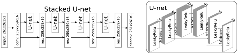
Fig. 1: The architecture of stacked U-net that consists of four residual U-net blocks. The right panel shows the U-net structure, and the depth of the hidden layer is denoted on the top of them.

2 Method

The training and testing data sets for deep learning are generated from traditional hydrodynamic simulations. For simplicity, we implemented (2+1)-d ideal hydrodynamics with zero viscosity and charge densities, using the code VISH2+1 with an ideal equation of state EoS $p=\frac{e}{3}$ [8]. The initial energy density profiles are generated by some initial condition models, such as MC-Glauber [9, 10], MC-KLN [10, 11], AMPT [12] and TRENTo [13] with zero transverse flow velocity. We run VISH2+1 at three fixed evolution times $\tau-\tau_{0}=2.0,\ 4.0,\ 6.0\ \mathrm{fm/c}\ (\tau_{0}=0.6\mathrm{fm/c})$ to obtain the final energy momentum tensor profiles $T^{\tau\tau}(\tau,x,y),T^{\tau x}(\tau,x,y),T^{\tau y}(\tau,x,y)$. The time step and grid size of the simulations are set to $d\tau=0.04\ \mathrm{fm/c}$ and $dx=dy=0.1\ \mathrm{fm}$ within a fixed transverse area of $13\ \mathrm{fm}\times 13\ \mathrm{fm}$.

The designed neural network, called stacked U-net(sU-net), belongs to the encoder-decoder network architecture, which could enhance the gradient flow in the deep part of the network during back propagation. As shown in Fig. 1, it contains four U-net blocks in series with residual connection. Inside each U-net block, there are three convolutional and deconvolutional layers, and the outputs of the first two convolutional layers are also fed into the last two deconvolutional ones through concatenating the feature maps along the channel dimension, respectively. The activation functions for all layers, except for the output one, are Leaky ReLU $f\left(x\right)=\max\left\{{x,0.03x}\right\}$. While the ones for the output layer are softplus $f\left(x\right)=\ln\left({1+{e^{x}}}\right)$ for $T^{\tau\tau}$ and $f(x)=1$ for $T^{\tau x}$ and $T^{\tau y}$. The kernel size of all layers is $3\times 3$, and the loss function is normalized MSE loss, $Loss=\frac{\|y_{1}-y_{0}\|^{2}}{\|y_{0}\|^{2}}$, where $y_{1}$ is the output of the network and $y_{0}$ is the ground truth. We minimize the loss function with the standard mini-batch stochastic gradient descent algorithm with batch size selected as 16 and a learning rate exponentially decaying from $10^{-3}$ to $10^{-5}$.

In practice, we divide the whole evolution time $\tau-\tau_{0}=6.0\ \mathrm{fm/c}$ into three parts with equal time interval $\Delta\tau=2.0\mathrm{fm/c}$, and train three individual sU-net for each part. After that, we use the trained sU-net-1 to predict the profiles at $\tau-\tau_{0}=2.0\mathrm{fm/c}$, and use them as initial conditions for sU-net-2 to predict the profiles at $\tau-\tau_{0}=4.0\mathrm{fm/c}$, and then use sU-net-3 to predict the final profiles at $\tau-\tau_{0}=6.0\ \mathrm{fm/c}$ (please refer to [6] for details).

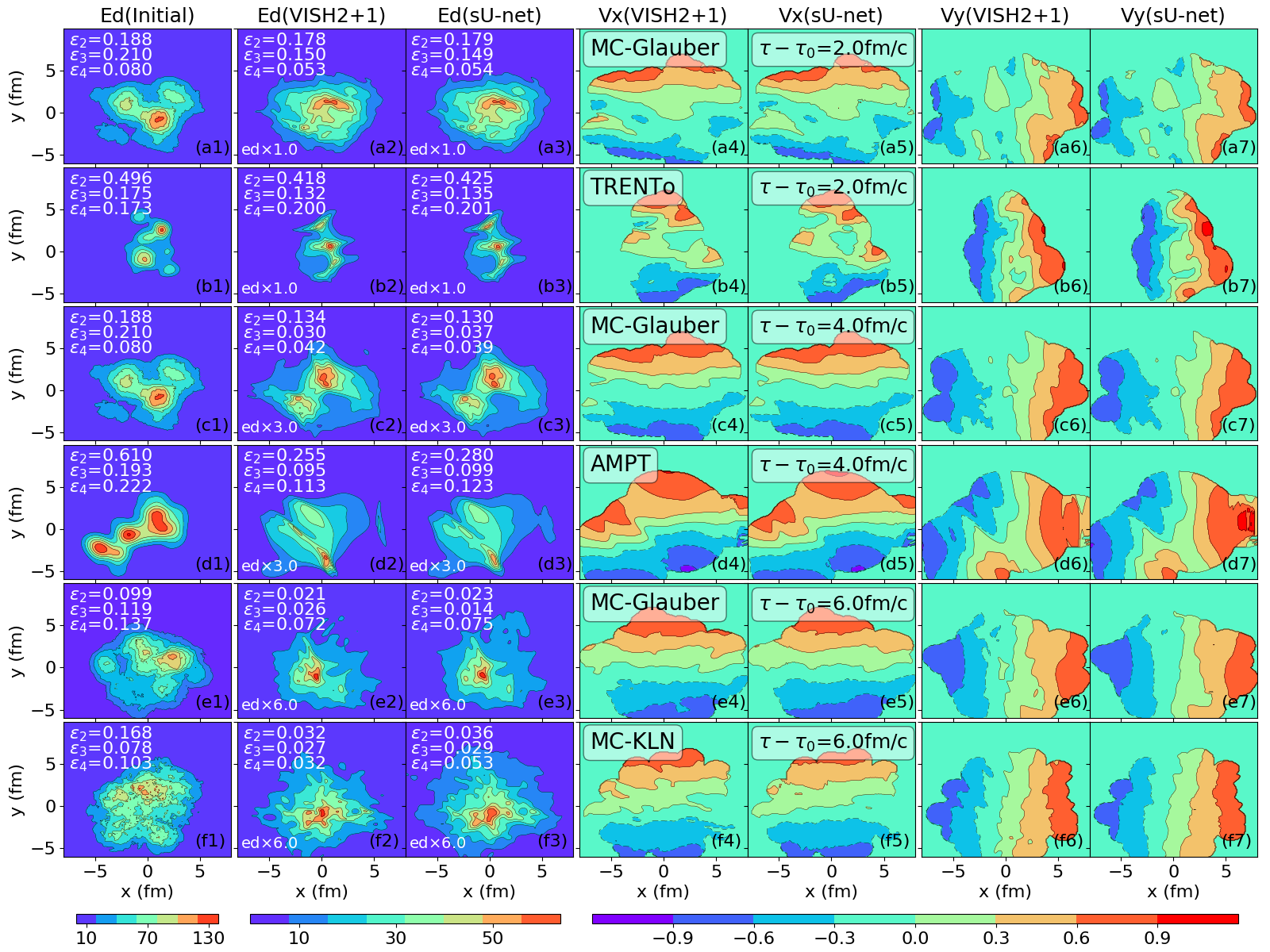
Fig. 2: Energy density and flow velocity profiles at $\tau-\tau_{0}=2.0,\ 4.0,\ 6.0\ \mathrm{fm/c}$, calculated from VISH2+1 and predicted by Stacked U-Net for six test cases with initial profiles generated from MC-Glauber, MC-KLN, AMPT and TRENTo.

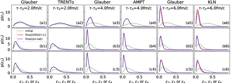
Fig. 3: Eccentricity distribution $P(\varepsilon_{n})$ (n=2, 3, 4), at $\tau-\tau_{0}=2.0,\ 4.0,\ 6.0\ \mathrm{fm/c}$, calculated from VISH2+1 and predicted by Stacked U-Net for 100000 tested initial profiles generated from MC-Glauber, MC-KLN, AMPT and TRENTo.

3 Results

The network sU-net is trained with 10000 initial and final profiles from VISH2+1 simulations with MC-Glauber initial conditions, and then tested on making predictions for the final profiles of four different types of initial conditions, including MC-Glauber, MC-KLN, AMPT and TRENTo. Fig. 2 shows the comparison between hydrodynamic results and the network predictions on final energy density and flow velocity at $\tau-\tau_{0}=2.0,\ 4.0,\ 6.0\ \mathrm{fm/c}$. It shows that the trained network is able to capture the magnitudes and structures of the contour plots of both energy density and flow velocity. Meanwhile, panel (b), (d) and (f) also show that sU-net, trained with data sets associated with the MC-Glauber initial conditions, can also nicely predict the final profiles of other initial conditions.

We also calculate the the eccentricity coefficients for the energy density profiles, $\varepsilon_{n}=\frac{\int r^{n}drd\phi e(r,\phi)e^{in\phi}}{\int r^{n}drd\phi e(r,\phi)}\ \ \ (n=2,3,4)$, which helps to evaluate the deformation and inhomogeneity of the QGP fireball. These true and predicted values of $\varepsilon_{n}$ (n=2, 3, 4) from hydrodynamics and network are written in the related panels(a-f).

Fig. 3 presents the eccentricity distributions $P(\varepsilon_{n})$ of energy density at $\tau-\tau_{0}=2.0,\ 4.0,\ 6.0\ \mathrm{fm/c}$, which shows that the results from the network almost overlap with the ones from VISH2+1 and are also obviously deviated from the initial eccentricity distributions $P_{0}(\varepsilon_{n})$. To further evaluate the accuracy of the network predictions, we plot the histograms of the true vs. predicted eccentricity $\varepsilon_{n}$ at $\tau-\tau_{0}=2.0,\ 4.0,\ 6.0\ \mathrm{fm/c}$, calculated from VISH2+1 and predicted by stacked U-Net for 100000 tested initial profiles generated from MC-Glauber, MC-KLN, AMPT and TRENTo. The prediction accuracy is very good at shorter evolution time $\tau-\tau_{0}=2.0\ \mathrm{fm/c}$, but gradually decreases for longer evolution time. Due to the limited memory of our local GPU server, we implement the combined sU-net series to predict the final profiles at longer evolution time, which also gradually accumulates errors with more sU-net added.

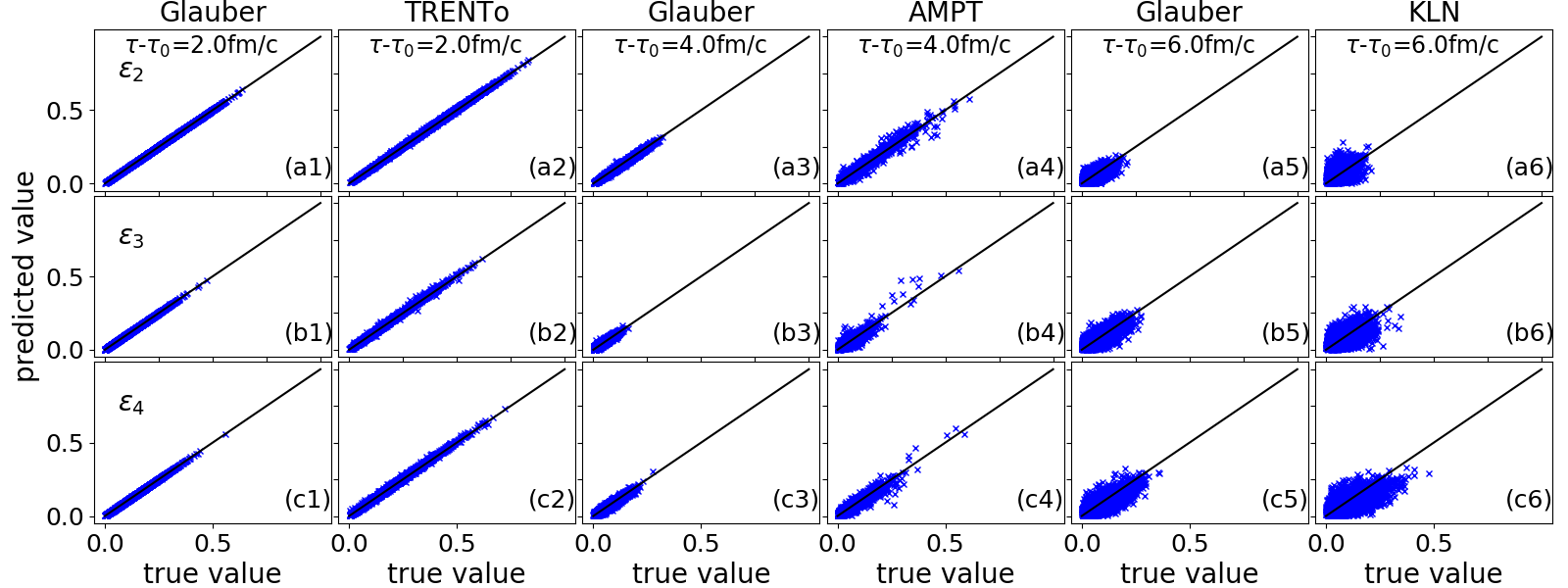
Fig. 4: Histograms of the true vs. predicted eccentricity $\varepsilon_{n}$ at $\tau-\tau_{0}=2.0,\ 4.0,\ 6.0\ \mathrm{fm/c}$, calculated from VISH2+1 and predicted by Stacked U-Net for 100000 tested initial profiles generated from MC-Glauber, MC-KLN, AMPT and TRENTo.

4 Conclusions

In this proceeding, we demonstrate that the well designed and trained neural network can capture the main features of the non-linear evolution of the relativistic hydrodynamics, which can not only predict the magnitude and inhomogeneous structures of the final profiles, but also describe the related eccentricity distributions $P(\varepsilon_{n})$ (n=2, 3, 4). We also noticed that prediction accuracy decreases with longer evolution time, which should be further improved with new designed network structure and more powerful GPU server.

5 Acknowledgments

We thank the discussions from L.G. Pang and K. Zhou. H. H, H. X. Z. W. and H. S. are supported by the NSFC and the MOST under grant Nos.11435001, 11675004 and 2015CB856900. B. X. and Y. M. are supported by grant no. 61772037.

References

- [1] Y. D. Hezaveh, L. Perreault Levasseur and P. J. Marshall, Nature 548, 555 (2017).
- [2] J. Carrasquilla and G. R. Melko, Nature Phys. 13, 431 (2017).
- [3] P. Baldi, P. Sadowski and D. Whiteson, Nature Commun. 5, 4308 (2014).
- [4] P. T. Komiske, E. M. Metodiev and M. D. Schwartz, JHEP 1701, 110 (2017).
- [5] L. G. Pang, K. Zhou, N. Su, H. Petersen, H. Stocker and X. N. Wang, Nature Commun. 9 no.1, 210, (2018).
- [6] H. Huang, B. Xiao, H. Xiong, Z. Wu, Y. Mu and H. Song, arXiv:1801.03334 [nucl-th].
- [7] U. Heinz and R. Snellings, Annu. Rev. Nucl. Part. Sci. 63, 123 (2013); C. Gale, S. Jeon and B. Schenke, Int. J. Mod. Phys. A 28, 1340011 (2013); H. Song, Y. Zhou and K. Gajdosova, Nucl. Sci. Tech. 28, no. 7, 99 (2017).
- [8] H. Song and U. W. Heinz, Phys. Rev. C 77, 064901 (2008).
- [9] M. L. Miller, K. Reygers, S. J. Sanders and P. Steinberg, Ann. Rev. Nucl. Part. Sci. 57, 205 (2007).
- [10] T. Hirano and Y. Nara, Phys. Rev. C 79, 064904 (2009).
- [11] H. J. Drescher and Y. Nara, Phys. Rev. C 75, 034905 (2007); Phys. Rev. C 76, 041903(R) (2007).
- [12] H. j. Xu, Z. Li and H. Song, Phys. Rev. C 93, no. 6, 064905 (2016).
- [13] J. S. Moreland, J. E. Bernhard and S. A. Bass, Phys. Rev. C 92, no. 1, 011901 (2015).