LineNet: a Zoomable CNN for Crowdsourced High Definition Maps Modeling in Urban Environments

Abstract

High Definition (HD) maps play an important role in modern traffic scenes. However, the development of HD maps coverage grows slowly because of the cost limitation. To efficiently model HD maps, we proposed a convolutional neural network with a novel prediction layer and a zoom module, called LineNet. It is designed for state-of-the-art lane detection in an unordered crowdsourced image dataset. And we introduced TTLane, a dataset for efficient lane detection in urban road modeling applications. Combining LineNet and TTLane, we proposed a pipeline to model HD maps with crowdsourced data for the first time. And the maps can be constructed precisely even with inaccurate crowdsourced data.

I Introduction

With the development of navigation and driving applications, HD maps are in increasing demand. Yet modeling HD maps was very expensive. Currently, there were two main ways to build HD maps. One is engineering surveying and mapping. The other is using special fleets and professional equipment[4, 20] (.e.g, HD camera, deep sensor, radar, etc.). Both of these methods require a large amount of manpower and resources. However, to construct detailed HD maps on a city scale, the higher coverage area is required so that it is necessary to reduce costs. To enlarge the coverage area and reduce costs, we developed a crowdsourced distribution system. In our system, data acquired on mobile phones by drivers could also be integrated into the model and increase coverage area. In addition to reducing costs, the crowdsourced strategy is also very convenient to extend and update. But it suffers from following restrictions.

• Due to the limitations of mobile devices, we can only obtain images and inaccurate GPS information.

• Images were captured by many drivers with unknown and different camera parameters.

• Images were sampled every 0.7 seconds by our crowdsourced app on the car due to the network bandwidth restriction. In an uneven speed, distance intervals of image sequences are different (usually 5-20 meters).

• Images of one road could be captured multiple times by different drivers.

Under these conditions, it is required to find a way to detect lanes accurately in a single image. Till now, there were only a few papers about road modeling [4, 20] and they did not consider crowdsourcing. So we proposed a road modeling system using crowdsourced images. First, we collect data in a crowdsourced way, then lane markings are detected using neural networks, finally we model HD maps using structure from motion (SfM) with the detection results.

As for lane detection, all roads and all of the lane markings cannot be obtained simultaneously by current methods. There are currently two types of approaches. One is based on road surface segmentation mostly for ego-lane[25, 6, 22]. However, these methods are affected by occlusions and the types of lane boundaries are ignored. The other is based on lane markings [13, 2, 3, 9, 15]. Lane markings contain more information, but they become narrower towards the vanishing points and finally converge, making it difficult to distinguish them.

To detect all roads and classify all the individual lane markings at the same time, we need a method which can capture both the global view and details. As deep convolutional neural networks(CNN) have shown great capability in lane detection [15, 9, 16, 14], we built a highly accurate CNN, named LineNet. To achieve high precision, a novel Line Prediction(LP) layer is included to locate lane markings directly instead of calculating from segmentation. In addition to the LP layer, the Zoom Module is added to recognize occlusion segments and gaps inside dashed lanes. With this module, the field of view (FoV) can be enlarged to arbitrary size without changing the network architecture. Combining these strategies together, LineNet can detect and classify lane markings across all roads. Details of LineNet will be discussed in Section IV.

Existing lane detection datasets are not effective enough for HD maps modeling. Necessary road boundaries and supportive occlusion area for HD maps modeling are not counted in existing dataset, including KITTI Road [8], ELAS dataset [2], Caltech Lanes Dataset [1], VPGNet Dataset [15], tuSimple lane challenge [26] and CULane[30]. Therefore, we build a new dataset with more than 10,000 images. In each image, comprehensive annotations for all roads including road boundaries, occlusions, 6 lane types and gaps inside dashed lines are extracted (see Table I). Details are in Section III.

TABLE I: Comparison of the KITTI road[8], ELAS[2], VPGNet Dataset[15], Caltech Lanes Dataset[1], tuSimple Lane Dataset [26], CULane[30] and our TTLane Dataset.

Datasets	Annotation type	Lane mark types	All roads	Road boundaries	Occlusion segments	Total amount
KITTI road[8]	segmentation	no	no	no	no	191
ELAS [2]	line	yes	no	no	no	$\approx$ 15000
Caltech Lanes Dataset[1]	line	yes	yes	no	no	1224
VPGNet Dataset[15]	line	yes	yes	no	no	$\approx$ 20000
tuSimple Lane Dataset[26]	line	no	yes	no	no	6408
CULane[30]	line	no	no	line	no	133235
TTLane Dataset	line	yes	yes	yes	partial(3000/13200)	13200

To test our method for HD maps modeling, we ran experiments in two steps: lane detection (Section V-A) and HD map modeling(Section V-B). The HD map modeling pipeline is composed of OpenSfM, LineNet, and some post processing. In the first step, LineNet was trained on different datasets and compared with the state-of-the-art techniques. It turned out that our approach outperformed other methods under various evaluation metrics. In the second step, our whole HD maps modeling pipeline was tested in a small-scale experiment. In this experiment, images and GPS information were collected with different transportations in three conditions(straight, turning, and crossroads). The ground truth of these roads was also collected. And HD maps was successfully constructed with crowdsourced data for the first time. Compared with the ground truth, our crowdsourced method can reduce the error to 31.3 cm, which is desirable.

In summary, our main contributions are as follows.

• We proposed LineNet, a CNN model consisting of an innovative Line Prediction Layer and Zoom Module, and achieved state-of-the-art performance on two main subtasks of lane detection.

• We developed TTLane Dataset, the most effective dataset for lane detection in road modeling applications.

• We proposed a pipeline to model HD maps with crowdsourced data for the first time and achieved great precision even when the crowdsourced data is very inaccurate.

II Related works

II-A Datasets

The KITTI road [8] dataset provides two types of annotation: segmentation of road and ego-lane. The road area is composed of all lanes where cars can drive. And the ego-lane area is the lane where the vehicle is currently driving. The ELAS dataset [2] also has ego-lane annotations, and Lane Mark Types(LMT) are annotated. More than 20 different scenes (in more than 15,000 frames) are provided in the ELAS dataset.

The Caltech Lanes Dataset [1] contains four video sequences taken at different times of the day in urban environments. It is divided into four sub-dataset and contains 1225 images in total. Lee et al. proposed VPGNet Dataset[15], consists of approximately 20,000 images with 8 lane marking types and 9 road mark types under four scenarios, different weather, and lighting conditions. Unlike the first two datasets, all lane markings of VPGNet Dataset are annotated. Another dataset is tuSimple lane challenge [26], that consists of 3626 training images and 2782 testing images taken on highway roads. CULane[30] currently is the biggest dataset about multiple lanes detection. But it is not designed for HD map modeling, as there is only annotations of the road currently being driven on and the annotations of road boundaries are missing.

Our dataset offers more considerable details than any existing dataset: LMTs are provided, and all lanes in the image are annotated. Furthermore, LMTs are more concise: white solid; white dash; yellow solid; yellow dash; and double lines are all included. Gaps inside dashed lines are also annotated. The differences among datasets are summarized in Table I and illustrated in Fig I.

Our dataset is the only dataset that offers annotations of road boundaries and occlusion segments. Road boundaries are necessary because lots of HD maps applications need them, and occlusion segments are useful for improving LineNet(Section V-C1). Annotations of road boundaries and separately labeled double lines make our TTLane Dataset a challenging large-scale dataset for lane detection in urban environments.

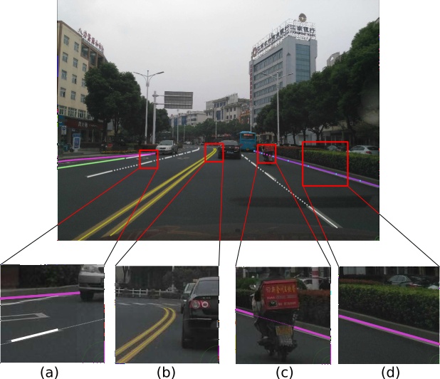
Figure 1: This figure shows annotations of our TTLane Dataset: (a). Annotation of dash lanes. (b). Annotation of double lanes. (c). Annotation of occlusion segments. (d). Annotation of road boundaries.

II-B Lane detection with CNN

Several papers about lane detection with CNN have been published in recent years [15, 9, 16, 14]. Lee et al. [15] proposed a multi-task CNN to detect lanes and road marks simultaneously. They achieved the best F1-score in the Caltech Lane dataset [1] because the vanishing point was used. He et al.[9] combined features from the front view and Birds-Eye-View for lane detection. Li et al. [16] extracted lane features from CNN, and fed them into a recurrent neural network, to utilize sequential contexts during driving. Máttyus et al. [20] used aerial images to improve the fine-grained segmentation result from ground view. Using the approach, they were able to recognize and model all roads. Liu et al.[18] proposed Dilated FPN with Feature Aggregation(DFFA) for drivable road detection. Chen and Chen[6] proposed RBNet to detect both road and road boundaries simultaneously. DFFA[18] and RBNet[6] achieved the best F1-score and precision respectively on the KITTI ego-lane segmentation task[8].

It is important for lane detectors to have a large field of view (FoV). For example, understanding large gaps inside dashed lanes requires the FoV to be larger than the length of the gap. Many researchers [5, 28, 29, 24, 21] have shown that large FoV can increase performance; Maggiori et al. [19] introduced several techniques for high-resolution segmentation. Chen et al.[5] used atrous convolution [23] and ResNet[10] to achieve larger FoV, and Wang et al. [27] proposed non-local blocks to gather global information from the CNN. Newell et al.[21] proposed stacked hourglass networks, to gather a global context during the multi-level hourglass process. Peng et al.[24] proposed a global convolutional network to enlarge the FoV. [28] proposed Zoom-in-Net that consists of three sub-networks. Low resolution images and high-resolution images are fed into two separate networks, and concatenated features are used for bounding box detection.

All of the methods mentioned above have some shortcomings for HD maps modeling. DFFA[18] and RBNet[6] predict the ego-lane segmentation, making LMTs lost. VPGNet[15] is hard to locate non-parallel lanes or lanes that are too close. [9, 16] and [20] require additional information such as perspective mapping. Our LineNet is designed to solve these issues.

TABLE II: Dataset Statistic. The meaning of these abbreviations is: WS(white solid), WD(white dash), RB(road boundaries), YS(yellow solid), YD(yellow dash)

width(px)	height(px)	images	WS	WD	RB	YS	YD	others	total
$2058\pm 163$	$1490\pm 215$	13200	24831	14136	22598	8945	2106	2613	75231

II-C HD Maps Modeling

There were only a few papers about HD Maps modeling[20, 31, 4]. Most of them have either[31, 4] or both[20] the following two characteristics: using aerial images[31] and with professional equipments[4]. Using aerial images to model HD Maps has a natural advantage, which is that the geographic location and topology of the maps are easy to construct. But it also has shortcomings: the road may be covered, or the resolution of aerial images is not enough for HD Maps modeling. With professional equipment(mount on the car), HD maps can be modeled precisely, but the costs are too high to detailedly model HD maps on a city scale. Street view is a related topic of HD maps, most companies (.e.g Google, HERE, Tencent, etc.) collect data with own fleets, but coverage is not high enough especially in rural and remote areas, the street view coverage of Tencent maps grows slowly in recent years, because the cost would be unacceptable if we want to enlarge the coverage. To detailedly model HD maps on a city scale, we choose the crowdsourced strategy. It can overcome the two shortcomings mentioned above without losing accuracy. We have developed a crowdsourced distribution system that allows drivers to collect data on mobile phones, and the HD maps can be updated without delay. It is worth mentioning that we can use those methods together, and our crowdsourced method can focus on regions where own fleets are hard to reach.

III TTLane Dataset

III-A Data Collection

Our dataset is crowdsourced. It was collected from different drivers(about 200), each with a phone camera mounted on the drivers’ dashboard. Because the dataset was obtained from different drivers’, phones, orientations, resolutions, exposures, focal lengths and so on, any algorithm should be robust to such variations. All images were collected in urban environments.

Most exist datasets are continuous video sequences because the temporal information can improve lane detection results. However, our dataset is different, TTLane has fewer overlapping parts, most of them are unordered. There are two reasons for this. First, the diversity of our dataset can be increased, the data can be collected from all over the world. Second, crowdsourcing suffers from the bandwidth of the mobile network, dense video sequences require more network traffic.

III-B Annotation

We manually annotated the center points of lane markings, Continuous lane markings are fitted and plotted with a Bezier curve. Each lane marking has a type. There are 6 types in total (white solid, white dash, yellow solid, yellow dash, road boundary, other). If there are double white solid lines in the road center, the annotator must draw 2 parallel white solid lines, which is shown in Fig 1. This annotation method can cope with complex double lane markings, such as left solid and right dashed lanes.

Annotations of occlusion segments and gaps inside dashed lanes are among other features of our dataset. Liang et al. [17] show that analysis of the occluded region can improve image segmentation performance, see more details in Section V-C1. So we annotated the occlusion segments with a dotted, continual lane. The same is true for gaps in dashed lanes. Note that we do not distinguish among occlusions and gaps – and they were annotated in the same format. As is shown in Fig 1.

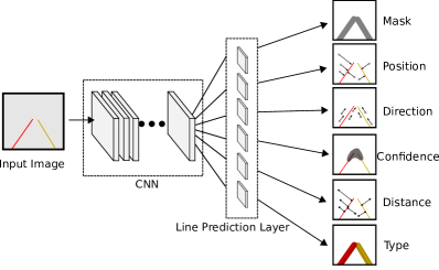
Figure 2: An illustration of the LP layer. LineNet will become confident when two lane markings are sufficiently far from each other.

III-C Dataset Statistics

Our dataset consists of 13200 images, 3000 of which were annotated with occlusion information and the rest of the 10200 images were usually annotated. Isolation belts, roadblocks and other things that may affect the road conditions were annotated as “other”. Regarding comprehensive annotation, our dataset is the most detailed and complicated dataset for road modeling in urban environments.

IV LineNet

IV-A Line Prediction Layer

Current lane detection investigations based on CNN were restricted to segmentation methods, which is not intuitive for line detection, causing inaccuracy. It is insufficient for real-life demands. Thus we propose a novel approach, that aims to provide new ideas for lane detection tasks.

We use a pre-trained ResNet model with dilated convolution[5] as the feature extractor. a dilated convolution strategy helps to increase receptive field, which is essential when detecting dashed lanes. To make the model suitable for the lane detection, we make two non-trivial extensions:

• An additional layer designed for lane positioning and classification, called the Line Prediction(LP) layer.

• A zoom module that automatically focuses on areas of interest, i.e., converging and intersection areas of the lane markings.

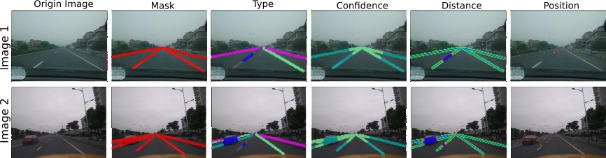
Figure 3: This figure shows different branches’ outputs of the LP layer, with two samples. The first column shows the original images. The second column shows the mask of the lanes. The background image in this row is much more blurred than the first column because this is what LineNet sees (i.e., the zoom level is 0.5 so we down-sample the input images). In the third column, different colors represent different lane marking types. Note the blue color represents the occlusion or gaps. In the fourth column, the light green color represents the unconfined area, and the cyan color represents the confident area where predictions are reliable. The fifth column represents the distance map from the anchor point to the center line. In the sixth column, we randomly sample some anchor points (blue points), and the green lines show the outputs of the position branch.

The Line Prediction (LP) layer is designed for accurate lane positioning and classification, inspired by Zhu et al.[32]’s three branch prediction procedure. There are six branches in our LP layer: line mask; line type; line position; line direction; line confidence; and line distance, as is shown in Fig 2.

A line mask is a stroke we draw with a fixed width (32 pixels in our experiments). The line type indicates one of the six-lane marking types. Line position predicts the vector from an anchor point to the closest point in the line. Supervising on the line position can produce much more accurate results than using a mask. Fig 3 illustrates this by showing that the line position branch can predict lanes in sub-pixel level. Line distance is the distance from the anchor point to the closest point in the line. Line direction predicts the orientation of the lane. Line confidence predicts the confidence ratio, i.e., whether the network can see the lane clear enough, which is defined between 0 (if two lines are closer than 46 pixels) and 1 (otherwise). When we zoom into two adjacent lines, they will gradually separates, result in change of the confidence ratio. We will discuss how do the six branches work together to predict a whole lane in Section IV-C. Figure 3 shows the supervised value in the LP layer with two examples.

IV-B Zoom Module

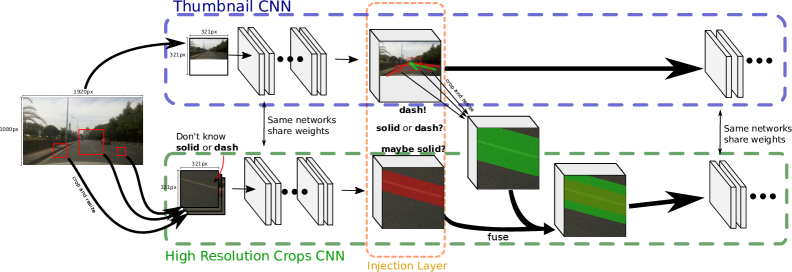
Figure 4: The Zoom Module fuses data from the thumbnail CNN and the high-resolution cropped CNN together, and detect a dashed lane in the high-resolution stream. The thumbnail CNN can recognize the dashed lane because it has larger FoV (field of view), while the high-resolution CNN accurately locates the lane markings.

The Zoom Module is the second feature of LineNet. With this module, LineNet can alter the FoV to an arbitrarily size without changing network structure. Our Zoom module is inspired by Zoom-in-Net [28] and non-local block [27]. It splits the data flow through the CNN into two streams: (i) a thumbnail CNN; and (ii) a high-resolution cropped CNN. Fig 4 illustrates the architecture of the Zoom Module. Fig 4 shows that the FoV depends on the size of the crops and thumbnails. A fixed network structure has lots of benefits, including effective use of pre-trained weights after Zoom Module is mounted, and fixed computational complexity.

The thumbnail CNN provides a global context for the features that the high-resolution CNN “sees” in detail. These two CNNs share weights and compute in parallel, up to a point where information from the “thumbnail” CNN is shared with the high-resolution CNN. Sharing is achieved via a layer we call the “injection layer”, that fuses features from both CNNs, and places the result in the data stream of the high-resolution CNN.

The Zoom Module and LP layer work together to boost performance. The zoom module allows the network to zoom into areas where the LP layer is not confident enough. In practice, the zooming procedure is used multiple times, with the zoom ratio gradually multiplied from 0.5 to 16. Fig 5 shows the four stages of the zooming process and how the LP layer and the zoom module interact with each other through the output of the line confidence branch. Overall, when the certainty of the lane rises, the spatial location of the lane becomes more accurate.

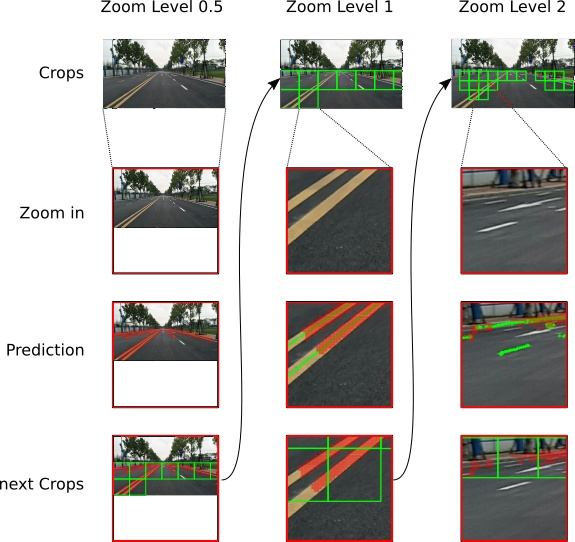
Figure 5: This figure illustrates the zooming process. Three columns represent three different zoom levels (more zoom levels can be added if necessary). The first row shows the high-resolution crops are fed into LineNet. The second row shows what LineNet sees in one crop. And the third row shows the prediction of LineNet in this crop. The red area represents the uncertain area. The fourth row represents crops that are generated for the next zoom level.

IV-C Post Processing

The results that LineNet detected were still discrete points. To achieve nice and smooth lines, points were clustered together and fitted into lines. The clustering algorithm named DBSCAN[7] was used with our hierarchical distance(HDis). The line position from the LP layer was collected and combined with a zoom level. The combination is denoted as a tuple $a=(x,y,z)$, where $(x,y)$ is the image coordinate from line position outputs, and $z$ is the stage’s zoom ratio used to predict the line position. We define the distance of two points, $a$ and $b$, in the equation 1. This distance was applied in DBSCAN clustering. And it allows DBSCAN to manipulate the appropriate distance from different zoom ratios.

$$HDis(a,b)=max(a.z,b.z)\sqrt{(a.x-b.x)^{2}+(a.y-b.y)^{2}}$$ (1)

After DBSCAN[7] clustering, line points of each cluster were fitted into a polynomial $p(x)=p_{0}+p_{1}x+p_{2}x^{2}+p_{3}x^{3}$, then smooth and reliable lines were achieved the and ready for evaluation. Fig 6 shows that the lane results are gradually clustered together during the zooming process.

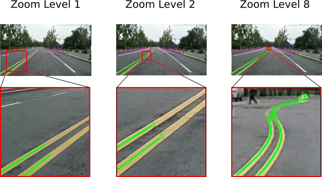
Figure 6: This figure illustrates that line points are gradually clustered together from near to far. Different colors represent different line types.

V Experiments

We divide our experiments into three subsections: 1. lane detection for HD maps modeling, that evaluates the effectiveness of our LineNet; 2. HD maps modeling, that analyzes the accuracy of our modeling pipeline; 3. Ablation studies.

V-A Lane Detection for HD Maps Modeling

There are two common subtasks in the lane detection task, which are: lane positioning and comprehensive lane detection. To prove the effectiveness of our method, we apply our model to the two subtasks and also compare our method with state-of-the-art approaches. The experiment of HD map modeling is described in Section V-B.

V-A1 Implementation Details

Our implementation is based on Tensorflow. We set the learning rate as the base learning rate multiplying $(1-\frac{iter}{iter_{max}})^{power}$; base learning rate is $2e^{-4}$, and the power is $0.9$. We use $0.9$ for momentum and $5e^{-4}$ weight decay. The number of training iterations varies due to different dataset sizes, but $80000$ iterations are sufficient for the three datasets with which we evaluate.

For the zoom module, we use the 66th layer (4b13) of the Dilated Resnet architecture [5] as the injection layer, Experiments showed that average fusion works well among various fusion methods.

V-A2 LineNet for Lane Positioning

In the lane positioning subtask, our goal is to predict all the lane markings in the image without considering their types. We use Caltech Lanes Dataset and our TTLane Dataset for this subtask. Caltech Lanes Dataset [1] contains 1225 images taken at different times of a day in urban environments. It is divided into four sub-datasets, cordova1, cordova2, washington1, and washington2, that contain 250, 406, 337 and 232 images respectively. We used the same training and testing set as in [15]. Our TTLane Dataset has up to 10K high-resolution finely annotated images taken in urban environments. We use 13000 images for training and validation and 200 images for testing and evaluation. Both datasets are annotated in a line-based way.

We adopted the method mentioned in [15], i.e., meaning we drew ground truth lines and predicted lines with a thickness of 40 pixels and evaluate the performance in a pixel-based way using F1-score measure.

We also adopted the method mentioned in [30], they draw lane markings with widths equal to 30 pixels and calculate the IoU between ground truth and predictions, we consider 0.5 as the threshold with the F1-score measure.

TABLE III: Comparison of lane positioning.

Method	CULane	Method	Caltech Lanes	Method	TTLane
	F1-score		F1-score		F1-score	Precision	Recall
Ours	0.731	Ours	0.955	Ours	0.832	0.848	0.816
SCNN[30]	0.713	VPGNet[15]	0.866	Mask R-CNN[11]	0.708	0.764	0.660
		Caltech[1]	0.723	MLD-CRF[12]	0.412	0.556	0.327
				SCNN[30]	0.790	0.794	0.787

We compare our method with VPGNet[15], Mask R-CNN[11], SCNN[30] and MLD-CRF[12]. VPGNet was the state-of-art method for comprehensive lane detection. Mask R-CNN is one of the best-performed object detection methods. MLD-CRF uses a conditional random field to do line positioning, and it is considered one of the best-performed method that do not need training. And SCNN[30] won the 1st price in TuSimple lane detection challenge 2017[26]. Results are shown in Table III. Our method achieved the best performance, and the result even exceeded the prior best performance by a substantial margin. This achievement reflects that our method works very well in line positioning.

V-A3 LineNet for Comprehensive Lane Detection

In this subtask, we need to predict both lanes marking positions and their types. It is the most difficult subtask of all two subtasks we did experiments on, especially in complex scenes where there are moving vehicles and other actions.

Our TTLane Dataset is a more challenging dataset for up to 6 different line types. We used 13000 images for training and validation, and 200 images for testing and evaluation, as is in the line positioning subtask. Unlike the metrics we mentioned above, here we evaluate area and distance between lines, not masks. We adopted a method that is similar to the one in [1]. Consider the ground truth line as gtLine and the prediction result as pdLine. The prediction result is considered correct when both of the following two conditions are met:

• The distance between the endpoints of two lines is smaller than a certain threshold (annotated as disThresh).

• The area enclosed by two lines is smaller than a certain threshold (annotated as areaThresh).

The metric in a way is just a representation of how close two lines are, as is shown in Fig 7. In our experiments, disThresh is set to 40px due to the high-resolution of images and areaThresh is set to disThresh times the length of gtLine.

Figure 7: This figuration visualizes the evaluation error. The red line is the ground truth, and the blue line is the prediction result to be evaluated. The second example mismatched because the distance between endpoints is too far, the third example mismatched because the area(gray part) between two lines are too large.

We also provided two different evaluation settings: ego-road (i.e., the road that the vehicle is currently driving on) evaluation and all roads evaluation. Ego-road evaluation only considers lane markings on the ego-road, while all roads evaluation considers all lane markings. Differences among ego-lane, ego-road, and all roads are shown in Fig 8.

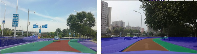
Figure 8: Differences between ego-lane(red), ego-road(green and red), and all roads(blue, green and red).

LineNet was compared with three state-of-the-art methods(Mask R-CNN[11], MLD-CRF[12], and SCNN[30]) on the two settings, i.e., ego-road evaluation and all roads evaluation. We did not compare the method with VPGNet[15] because the vanishing points are not annotated in our dataset. Results are shown in Table IV. Our method achieved the best performance on all evaluation metrics.

TABLE IV: Comparison of comprehensive lane detection.

Method	ego-road			all roads
	F1	PRE	REC	F1	PRE	REC
Mask R-CNN[11]	0.568	0.580	0.556	0.521	0.538	0.506
MLD-CRF[12]	0.206	0.260	0.171	0.193	0.267	0.150
SCNN[30]	0.608	0.594	0.623	0.560	0.537	0.585
Ours	0.708	0.651	0.778	0.663	0.613	0.722

To intuitively show the advantages of LineNet, here in Fig 9 some prediction results on the testing set are shown. These results were compared to Mask R-CNN[11] and MLD-CRF[12] and SCNN[30]. As is shown in column 1-3, due to the benefit of zoom module, LineNet can predict double lines as two separate lines, while Mask-RCNN and SCNN cannot. In column 3, we can see clearly that LineNet does well on the curve on the remote side (yellow lines), while Mask R-CNN and MLD-CRF just hold the line straight. In column 4, LineNet can still work well in the rural environment, however, MLD-CRF breaks down. We can conclude from the experiment that mask-based lane detection, like Mask R-CNN and SCNN, cannot handle details well, like double line detection very well. Methods like MLD-CRF that don’t need training can hardly perform well in complex scenes.SCNN[30] and MLD-CRF[12] do not produce classes information, so the classes with all methods were evaluated except these two. By contrast, LineNet was robust and performed well in both situations.

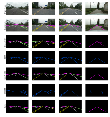
Figure 9: Visual compression on TTLane testing set. LineNet performs better in double lines and line direction on the remote side.

V-B HD Map Modeling

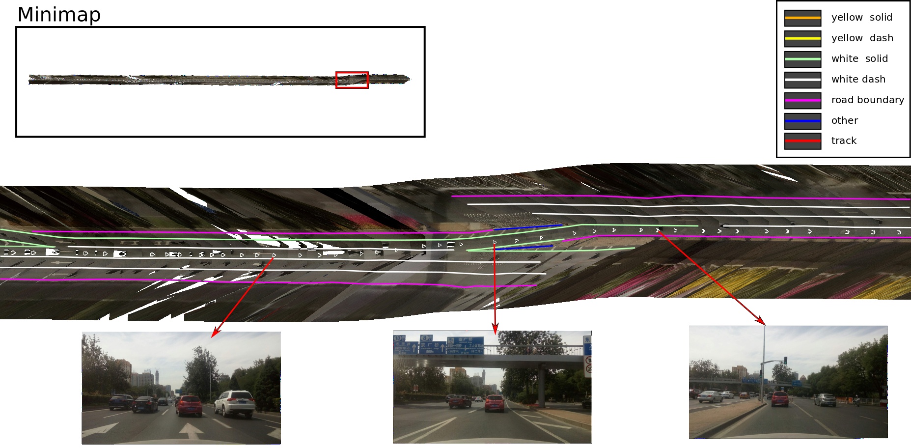
(a) This sub figuration showed road modeling results in lane changed. As you can see, our method can model the ramp and multiple lanes.

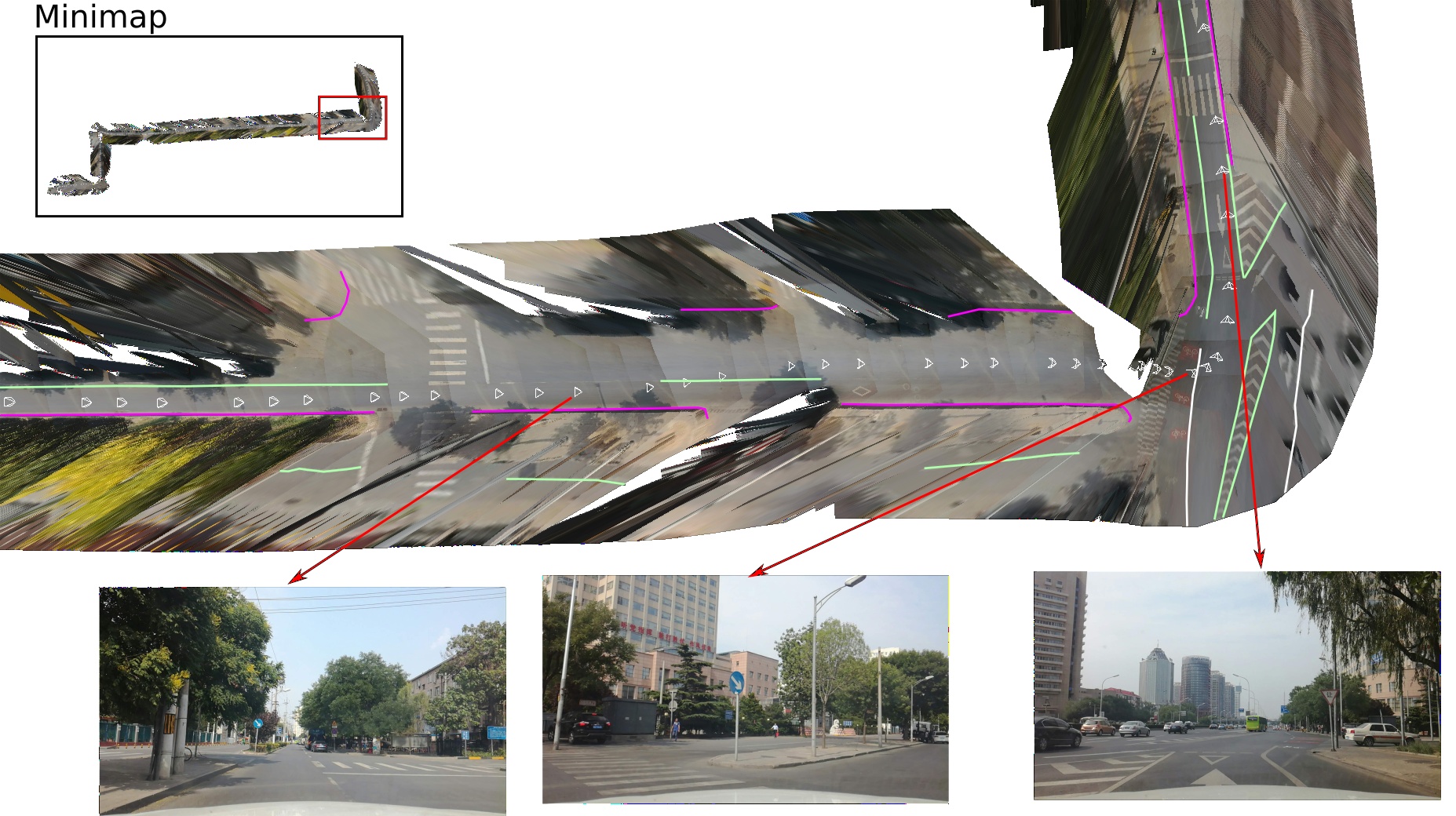
(b) This sub figuration showed road modeling results in turning. SfM is stabled when turning, and the road modeling results were still clean and well matched.

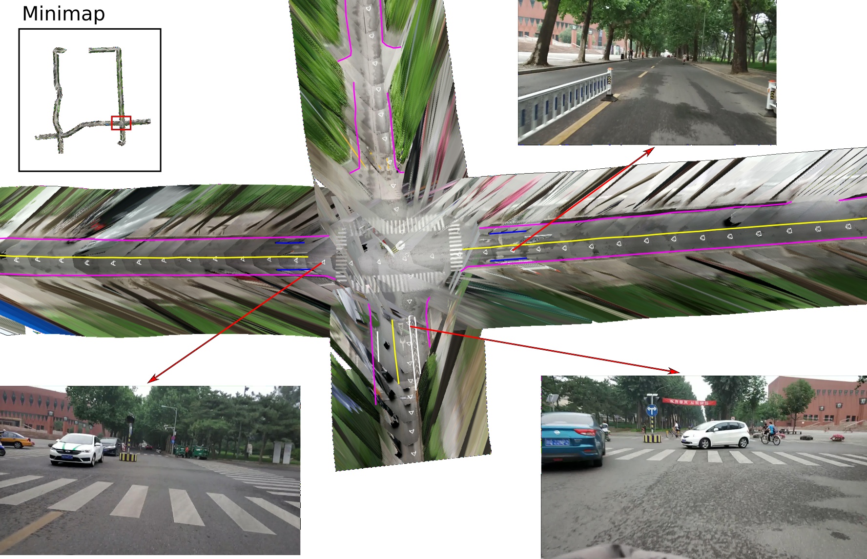
(c) This sub figuration showed road modeling results in crossroads. This data collected from three different transportation. In the zooming area, two drivers passed crossroad in different directions. SfM can stitch this two road together and yield self-conform results.

Figure 10: This three sub figurations showed how our road modeling algorithm works on three common road conditions. Each sub figurations contained a mini-map and a zooming area, the red box in the mini-map indicated the location of the zooming area. In the zooming area, the road modeling results were shown with colored lines. Each white triangle represented a shot position. The interval between two shots is about 5-20 meters, because of the limitation of bandwidth. Note: We did not use any additional data(such as satellite image) except images and GPS, the ground surface images were stitch from crowdsourced data.

To test our pipeline for HD maps modeling, we ran a small scale experiment and successfully constructed HD maps with inaccurate data. This pipeline consists of OpenSfM, LineNet and some post-processing. In this experiment, images and GPS information were collected with different transportations (cars, bicycles, electric bikes) in three road conditions (straight, turning, and crossroads). These transportations were driven by three riders. These riders covered different sections of the road and overlapped with each other. Images were collected at intervals of 5-20 meters, combined with inaccurate GPS information (with errors about 5 meters). HD maps were successfully constructed with our pipeline. It was found that the SfM is well connected to the overlapping parts and the post-processing converted detection results to smooth and reliable lines. Ground truth of these roads was also collected. Compared with the ground truth, our crowdsourced method can reduce the error to about 31.3 cm. It is worth mentioning that although the GPS error of mobile devices is large, the method can still reduce the error to a small amount.

In this section, two kinds of error measurement are used: ground surface parameters reconstruction error, that reflects the error of using SfM to rebuild the ground surface, and lane error, that reflects the lane offset with the ground truth.

V-B1 Ground Surface Parameters Reconstruction

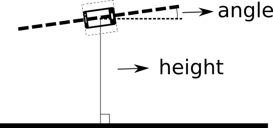
Figure 11: Ground Surface Parameters consist of angle and height. Angle parameter is the angle between the horizontal line of the mobile phone and the ground. Height parameter is the distance between the mobile phone and the ground.

Compared with the original GPS information, using SfM can reconstruct more accurate camera movement. But the road surface is still unknown. To construct the road surface, we segmented the point cloud obtained by SfM, and fit all the ground point clouds to a surface with ground surface parameters. Then the surface was used as the ground. Ground Surface Parameters(GSPs) consist of angle and height(showed in Fig 11), we solved the GSPs for each shot position, Table V showed our GSPs reconstruction error in three different road conditions. These three road conditions were shown in Fig 10.

TABLE V: GSP reconstruction error

Data	Shots Number	Average Height Error	Average Rotation Error
straight	173	0.15 meters	5 degrees
turning	342	0.11 meters	8 degrees
crossroad	1476	0.23 meters	9 degrees

V-B2 Lane Merging

The lanes that LineNet detected were still fragmented. There is no correlation between shots. To model entire lanes, these detection results were projected into the road surface, and they were merged by the same method we mentioned in Section IV-C. Fig 10 shows the lanes were merged in three different road conditions. To verify our lane merging results, we evaluated our result to the ground-truth which collected from laser sensors. Evaluate method is the same with Section V-A3. The average evaluation error is 31.3 cm. This is a significant improvement because the GPS error of our mobile devices is about 5 meters.

The HD map modeling experiment is still small due to our limited resources. We plan to model a city-scale HD maps and release it into a mobile phone application for everyone.

V-C Ablation Study

V-C1 Training with Occlusion Segments Improves Accuracy

Lane marks can be blocked by moving vehicles and thus be incomplete. We call the blocked parts of the mark “occlusion segments”. Our TTLane Dataset annotates occlusion segments. To inspect the effect of occlusion segments. LineNet was trained under two conditions. one is to treat occluded segments as normal lane markings, called “training without occlusion segments”. Another is to treat them as a special type of lines, called “training with occlusion segments”. Results are shown in Table VI. The experiment showed that training with occlusion segments performed better.

TABLE VI: Comparison on Ablation Study for Occlusion Segments

Strategy	F1-score	Precision	Recall
without occlusion segments	0.637	0.553	0.753
with occlusion segments	0.708	0.651	0.778

V-C2 Zoom Module Improves Precision

TABLE VII: Comparison on Ablation Study for Occlusion Segments

Strategy	F1-score	Precision	Recall
without zoom modules	0.634	0.525	0.801
with zoom modules	0.708	0.651	0.778

In this experiment, we canceled the feature fusion process of the zoom module, resulting in that the global features of the thumbnail net cannot be transmitted to the high-resolution crops net. We found that the feature fusion process significantly improved precision, but the recall had a slight decrease. The F1-score was improved with the results appearing in the Table VII.

V-C3 The Influences of each branch in LP layer

In this experiment, we separated the different branches, including position branch, direction branch, distance branch, and confidence branch. The position branch produces more accurate results. When we use the disThres of 40 pixels, the F1-score was only slightly improved by the position branch. But when the disThres was set to 10 pixels, using the position branch significantly improved the effect(Table VIII).

Both the direction branch and the distance branch improve the convergence speed during the training process. In 10,000 steps, the training loss is about 10% smaller when the two branches were used. And using this two branches does not affect the F1-score of final result.

The confidence branch is necessary for increasing the F1-score. When we removed the confidence branch, the zooming process also turned off because it depends on the result of the confidence branch, so the network will only see the image in the first stage. And the F1-score was greatly reduced.

TABLE VIII: Comparison on Ablation Study for each branches

Strategy	F1-score	Precision	Recall	F1-score(10px)
without position branch	0.697	0.643	0.762	0.627
without direction branch	0.703	0.647	0.771	0.673
without distance branch	0.696	0.640	0.763	0.670
without confidence branch	0.615	0.554	0.693	0.531
with all branches	0.708	0.651	0.778	0.682

VI Conclusion

In this paper, we propose LineNet and the TTLane dataset, both of which help us capture the lane and road boundary for crowdsourced HD maps modeling. For the first time, we propose a pipeline to model HD Maps with crowdsourced data our method achieves great precision even with inaccurate data. The method also shows the ability to model HD maps accurately without special equipment. Therefore our method can enlarge the coverage area of HD maps efficiently.

References

- Aly [2008] Mohamed Aly. Real time detection of lane markers in urban streets. In Intelligent Vehicles Symposium, 2008 IEEE, pages 7–12. IEEE, 2008.
- Berriel et al. [2017] Rodrigo F Berriel, Edilson de Aguiar, Alberto F de Souza, and Thiago Oliveira-Santos. Ego-lane analysis system (elas): Dataset and algorithms. Image and Vision Computing, 68:64–75, 2017.
- Beyeler et al. [2014] Michael Beyeler, Florian Mirus, and Alexander Verl. Vision-based robust road lane detection in urban environments. In Robotics and Automation (ICRA), 2014 IEEE International Conference on, pages 4920–4925. IEEE, 2014.
- Bittel et al. [2017] Sebastian Bittel, Timo Rehfeld, Michael Weber, and Johann Marius Zöllner. Estimating high definition map parameters with convolutional neural networks. 2017 IEEE International Conference on Systems, Man, and Cybernetics (SMC), pages 52–56, 2017.
- Chen et al. [2017] Liang-Chieh Chen, George Papandreou, Iasonas Kokkinos, Kevin Murphy, and Alan L. Yuille. Deeplab: Semantic image segmentation with deep convolutional nets, atrous convolution, and fully connected crfs. IEEE transactions on pattern analysis and machine intelligence, 2017.
- Chen and Chen [2017] Zhe Chen and Zijing Chen. Rbnet: A deep neural network for unified road and road boundary detection. In International Conference on Neural Information Processing, pages 677–687. Springer, 2017.
- Ester et al. [1996] Martin Ester, Hans-Peter Kriegel, Jörg Sander, Xiaowei Xu, et al. A density-based algorithm for discovering clusters in large spatial databases with noise. In Kdd, volume 96, pages 226–231, 1996.
- Fritsch et al. [2013] Jannik Fritsch, Tobias Kuhnl, and Andreas Geiger. A new performance measure and evaluation benchmark for road detection algorithms. In Intelligent Transportation Systems-(ITSC), 2013 16th International IEEE Conference on, pages 1693–1700. IEEE, 2013.
- He et al. [2016a] Bei He, Rui Ai, Yang Yan, and Xianpeng Lang. Accurate and robust lane detection based on dual-view convolutional neutral network. In Intelligent Vehicles Symposium (IV), 2016 IEEE, pages 1041–1046. IEEE, 2016a.
- He et al. [2016b] Kaiming He, Xiangyu Zhang, Shaoqing Ren, and Jian Sun. Deep residual learning for image recognition. In Proceedings of the IEEE conference on computer vision and pattern recognition, pages 770–778, 2016b.
- He et al. [2017] Kaiming He, Georgia Gkioxari, Piotr Dollár, and Ross Girshick. Mask r-cnn. In Computer Vision (ICCV), 2017 IEEE International Conference on, pages 2980–2988. IEEE, 2017.
- Hur et al. [2013] Junhwa Hur, Seung-Nam Kang, and Seung-Woo Seo. Multi-lane detection in urban driving environments using conditional random fields. In Intelligent Vehicles Symposium (IV), 2013 IEEE, pages 1297–1302. IEEE, 2013.
- Jung et al. [2013] Heechul Jung, Junggon Min, and Junmo Kim. An efficient lane detection algorithm for lane departure detection. In Intelligent Vehicles Symposium (IV), 2013 IEEE, pages 976–981. IEEE, 2013.
- Kim and Park [2017] Jiman Kim and Chanjong Park. End-to-end ego lane estimation based on sequential transfer learning for self-driving cars. In Computer Vision and Pattern Recognition Workshops (CVPRW), 2017 IEEE Conference on, pages 1194–1202. IEEE, 2017.
- Lee et al. [2017] Seokju Lee, Junsik Kim, Jae Shin Yoon, Seunghak Shin, Oleksandr Bailo, Namil Kim, Tae-Hee Lee, Hyun Seok Hong, Seung-Hoon Han, and In So Kweon. Vpgnet: Vanishing point guided network for lane and road marking detection and recognition. In Computer Vision (ICCV), 2017 IEEE International Conference on, pages 1965–1973. IEEE, 2017.
- Li et al. [2017] Jun Li, Xue Mei, Danil Prokhorov, and Dacheng Tao. Deep neural network for structural prediction and lane detection in traffic scene. IEEE transactions on neural networks and learning systems, 28(3):690–703, 2017.
- Liang et al. [2016] Xiaodan Liang, Yunchao Wei, Xiaohui Shen, Zequn Jie, Jiashi Feng, Liang Lin, and Shuicheng Yan. Reversible recursive instance-level object segmentation. In Proceedings of the IEEE Conference on Computer Vision and Pattern Recognition, pages 633–641, 2016.
- Liu et al. [2017] Xiaolong Liu, Zhidong Deng, and Guorun Yang. Drivable road detection based on dilated fpn with feature aggregation. In Proceedings of the IEEE International Conference on Tools with Artificial Intelligence, 2017.
- Maggiori et al. [2017] Emmanuel Maggiori, Yuliya Tarabalka, Guillaume Charpiat, and Pierre Alliez. High-resolution semantic labeling with convolutional neural networks. IEEE Transactions on Geoscience and Remote Sensing, 2017.
- Máttyus et al. [2016] Gellért Máttyus, Shenlong Wang, Sanja Fidler, and Raquel Urtasun. Hd maps: Fine-grained road segmentation by parsing ground and aerial images. In Proceedings of the IEEE Conference on Computer Vision and Pattern Recognition, pages 3611–3619, 2016.
- Newell et al. [2016] Alejandro Newell, Kaiyu Yang, and Jia Deng. Stacked hourglass networks for human pose estimation. In European Conference on Computer Vision, pages 483–499. Springer, 2016.
- Oliveira et al. [2016] Gabriel L Oliveira, Wolfram Burgard, and Thomas Brox. Efficient deep models for monocular road segmentation. In Intelligent Robots and Systems (IROS), 2016 IEEE/RSJ International Conference on, pages 4885–4891. IEEE, 2016.
- Papandreou et al. [2015] George Papandreou, Iasonas Kokkinos, and Pierre-André Savalle. Modeling local and global deformations in deep learning: Epitomic convolution, multiple instance learning, and sliding window detection. In Computer Vision and Pattern Recognition (CVPR), 2015 IEEE Conference on, pages 390–399. IEEE, 2015.
- Peng et al. [2017] Chao Peng, Xiangyu Zhang, Gang Yu, Guiming Luo, and Jian Sun. Large kernel matters - improve semantic segmentation by global convolutional network. In CVPR, 2017.
- Teichmann et al. [2016] Marvin Teichmann, Michael Weber, Johann Marius Zöllner, Roberto Cipolla, and Raquel Urtasun. Multinet: Real-time joint semantic reasoning for autonomous driving. CoRR, abs/1612.07695, 2016.
- [26] TuSimple. Tusimple lane detection challenge. Computer Vision and Pattern Recognition Workshops (CVPRW), 2017 IEEE Conference.
- Wang et al. [2018] Xiaolong Wang, Ross Girshick, Abhinav Gupta, and Kaiming He. Non-local neural networks. Proceedings of the IEEE Conference on Computer Vision and Pattern Recognition, 2018.
- Wang et al. [2017] Zhe Wang, Yanxin Yin, Jianping Shi, Wei Fang, Hongsheng Li, and Xiaogang Wang. Zoom-in-net: Deep mining lesions for diabetic retinopathy detection. In International Conference on Medical Image Computing and Computer-Assisted Intervention, pages 267–275. Springer, 2017.
- Xia et al. [2016] Fangting Xia, Peng Wang, Liang-Chieh Chen, and Alan L Yuille. Zoom better to see clearer: Human and object parsing with hierarchical auto-zoom net. In European Conference on Computer Vision, pages 648–663. Springer, 2016.
- Xingang Pan and Tang [2018] Ping Luo Xiaogang Wang Xingang Pan, Jianping Shi and Xiaoou Tang. Spatial as deep: Spatial cnn for traffic scene understanding. In AAAI Conference on Artificial Intelligence (AAAI), February 2018.
- Zang et al. [2017] Andi Zang, Runsheng Xu, Zichen Li, and David Doria. Lane boundary extraction from satellite imagery. In AutonomousGIS@SIGSPATIAL, 2017.
- Zhu et al. [2016] Zhe Zhu, Dun Liang, Songhai Zhang, Xiaolei Huang, Baoli Li, and Shimin Hu. Traffic-sign detection and classification in the wild. In Proceedings of the IEEE Conference on Computer Vision and Pattern Recognition, pages 2110–2118, 2016.