Cross-correlations between scalar perturbations
and magnetic fields
in bouncing universes
Abstract
Bouncing scenarios offer an alternative to the inflationary paradigm for the generation of perturbations in the early universe. Recently, there has been a surge in interest in examining the issue of primordial magnetogenesis in the context of bouncing universes. As in the case of inflation, the conformal invariance of the electromagnetic action needs to be broken in bouncing scenarios in order to generate primordial magnetic fields which correspond to observed strengths today. The non-minimal coupling, which typically depends on a scalar field that possibly drives the homogeneous background, leads to a cross-correlation at the level of the three-point function between the perturbation in the scalar field and the magnetic fields. This has been studied in some detail in the context of inflation and, specifically, it has been established that the three-point function satisfies the so-called consistency relation in the squeezed limit. In this work, we study the cross-correlation between the magnetic fields and the perturbation in an auxiliary scalar field in a certain class of bouncing scenarios. We consider couplings that lead to scale invariant spectra of the magnetic field and evaluate the corresponding cross-correlation between the magnetic field and the perturbation in the scalar field. We find that, when compared to de Sitter inflation, the dimensionless non-Gaussianity parameter that characterizes the amplitude of the cross-correlations proves to be considerably larger in bouncing scenarios. We also show that the aforementioned consistency condition governing the cross-correlation is violated in the bouncing models. We discuss the implications of our results.
1 Introduction
Magnetic fields permeate the universe over a wide range of scales. In addition to the detection of magnetic fields in astrophysical systems such as stars and galaxies, recent observations also point towards the prevalence of these fields on cosmological scales, viz. in the large scale structures [1, 2, 3, 4, 5, 6] and even in the intergalactic medium [7, 8]. In galaxies and clusters of galaxies, the strengths of the magnetic fields have been measured to be a few micro Gauss, while in the intergalactic medium, they are estimated to be of the order of Gauss at Mpc [7, 8, 9, 10, 11, 12, 13, 14, 15, 16]. In contrast, using CMB observations by Planck and POLARBEAR, the upper bound on the magnetic fields has been arrived at to be about a few nano Gauss [17, 18], which has also been corroborated by the upper limits obtained from the NRAO VLA Sky Survey [19]. It is well known that certain astrophysical processes, particularly the dynamo mechanism, can, in the presence of a seed field, augment the strength of the magnetic fields in galaxies. The origin of such progenitor fields is usually attributed to primordial processes.
Inflation is presently the most widely accepted paradigm to explain the generation and evolution of perturbations in the early universe. The issue of magnetogenesis, viz. the origin of magnetic fields, has been widely studied in various inflationary scenarios and, by means of the breaking of conformal invariance of the electromagnetic field, it has been possible to obtain scale invariant magnetic fields of the relevant strengths over the correlation scales of interest [20, 21, 22, 23, 24, 25, 26, 27, 28, 29, 30, 31, 32, 33, 34, 35, 36, 37, 38]. Nevertheless, such models are known to be afflicted by the backreaction and strong coupling problems [23, 39, 40]. Consequently, it seems worthwhile to investigate the generation of magnetic fields in scenarios that provide a feasible alternative to the inflationary framework. Among such alternatives, the most popular ones are the so-called bouncing models [41, 42, 43, 44, 45, 46, 47, 48, 49, 50, 51, 52, 53, 54, 55, 56, 57, 58, 59, 60, 61]. In these models, the universe goes through a period of contraction followed by an expanding phase, with a ‘bounce’ connecting the two epochs. Lately, there have been some efforts towards understanding the generation of magnetic fields in the bouncing scenarios [62, 63, 64, 65, 66, 67, 68].
In a recent work [65], we had analytically illustrated how scale invariant magnetic fields can be produced in a certain sub-class of symmetric bouncing scenarios. Using these analytical solutions, it would be interesting to examine the cross-correlations of these magnetic fields with scalar perturbations present in the bouncing scenarios. These correlations have been examined before in the context of inflation [69, 70, 71, 72, 73]. The magnitude of the non-Gaussianities generated through such correlations has been estimated to be quite large for inflation, and the shape of the non-Gaussianities peaks in the flattened limit, i.e. when the wavenumber of the scalar perturbation is twice the wavenumber associated with the two modes of the magnetic field. In this work, we study the cross-correlations of the magnetic fields produced in bouncing universes with the perturbations in an auxiliary scalar field. Ideally, it would be more appropriate to evaluate the cross-correlation between the primordial magnetic fields and the curvature perturbation. However, as is well known, examining the behavior of the curvature perturbations in bouncing models necessitates considerable modeling, often involving more than one field (see, for instance, Ref. [74]). Therefore, it would be instructive to first investigate the behavior of the cross-correlation of the magnetic fields with the perturbation in an auxiliary scalar field and explore their ramifications.
One of the most important characteristics of three-point functions is their behavior in the squeezed limit of the wavenumbers involved, i.e. when one of the wavenumbers is assumed to be much smaller than the other two. In inflation, typically, the amplitude of the mode with the longest wavelength and, therefore, the smallest wavenumber, freezes on super-Hubble scales. Therefore, in the squeezed limit, the three-point function can be completely expressed in terms of the two-point function through a relation referred to as the consistency condition (see Refs. [75, 76, 77, 78, 79, 80, 81] in the context of three-point functions involving scalar and tensor perturbations, and Refs. [71, 72] for cross-correlations between the scalar perturbation and the magnetic fields). However, in the case of the bouncing models that we shall study, the amplitude of the scalar perturbations grows strongly as one approaches the bounce (in this context, see Refs. [82, 74]). This suggests that the consistency relation may not hold in such scenarios (for a similar effect in the case of the tensor bispectrum, see Ref. [82]). Therefore, it is of utmost significance to examine whether the consistency relation, which holds true for inflationary magnetogenesis, would be valid in the bouncing models.
This paper is organized as follows. In the following section, we shall describe a few essential aspects concerning the evolution of the electromagnetic field in the presence of non-minimal coupling. We shall also evaluate the power spectra of the magnetic fields that arise in inflationary as well as bouncing scenarios in the presence of a non-minimal, power law coupling that is often considered in this context. In Sec. 3, after briefly revisiting the calculation of the cross-correlations between the perturbation in the scalar field and the magnetic fields in the context of inflation, we shall evaluate the corresponding three-point function in the matter bounce scenario of our interest. In Sec. 4, we shall define a dimensionless non-Gaussianity parameter to characterize the three-point function and calculate the parameter in both the inflationary and bouncing models. In Sec. 5, we shall evaluate the cross-correlation in the squeezed limit and illustrate that, while the consistency relation holds true in the case of inflation, it is violated in the bouncing scenario. Finally, we shall conclude with a brief discussion in Sec. 6.
We shall work with natural units such that , and set the Planck mass to be . We shall adopt the metric signature of . Greek indices shall denote the spacetime coordinates, whereas the Latin indices shall represent the spatial coordinates, except for which shall be reserved for denoting the wavenumber. Lastly, an overprime shall denote differentiation with respect to the conformal time coordinate.
2 Generation of scale invariant magnetic fields in the early universe
In this section, we shall describe the generation of primordial magnetic fields via a non-minimal coupling. We shall introduce the form of the electromagnetic action and, after choosing to work in a specific gauge, we shall obtain the equation of motion governing the electromagnetic vector potential. We shall quantize the vector potential in terms of the modes that satisfy the equation of motion in Fourier space. We shall also define the power spectrum corresponding to the energy density associated with the magnetic field. Thereafter, we shall consider a certain form of the coupling function wherein it can be expressed as a simple power of the scale factor, and analytically evaluate the magnetic power spectra in de Sitter inflation and in a specific class of bouncing scenarios.
2.1 Non-minimally coupled electromagnetic fields
We shall consider the background to be the spatially flat, Friedmann-Lemaître-Robertson-Walker (FLRW) metric that is described by the line-element
| (2.1) |
where is the scale factor and denotes the conformal time coordinate. We shall consider the action
| (2.2) |
where the electromagnetic field tensor is given in terms of the vector potential by the relation
| (2.3) |
The quantity describes the non-minimal coupling, with denoting a scalar field that possibly contributes to the background evolution. We shall assume that there is no homogeneous component to the electromagnetic field. We shall choose to work in the Coulomb gauge wherein and . In such a gauge, at the quadratic order in the inhomogeneous modes, the action describing the electromagnetic field is found to be (see, for example, Ref. [24, 27])
| (2.4) |
We can vary this action to arrive at the following equation of motion for the electromagnetic vector potential:
| (2.5) |
For each comoving wavevector , we can define the right-handed orthonormal basis , where
| (2.6) |
On quantization, the vector potential can be Fourier decomposed as follows [24, 27]:
| (2.7) |
where the Fourier modes satisfy the differential equation
| (2.8) |
The quantities represent the polarization vectors and the summation corresponds to the two orthonormal transverse polarizations. The operators and are the annihilation and creation operators satisfying the following standard commutation relations:
| (2.9) |
Let us now define a new variable , which, as we shall see, proves to be convenient to deal with. In terms of the new variable, Eq. (2.8) for simplifies to
| (2.10) |
2.2 Power spectra
Since we shall be focusing only on the properties of the magnetic field and not those of the electric field, let us attend to the power spectra of the generated magnetic fields. Let denote the operator corresponding to the energy density associated with the magnetic field. Upon using the decomposition (2.7) of the vector potential, the expectation values of the energy density can be evaluated in the vacuum state, say, , that is annihilated by the operator for all and . It can be shown that the spectral energy density of the magnetic field can be expressed in terms of the modes and and the coupling function as follows [24, 27]:
| (2.11) |
The spectral energy density is often referred to as the power spectrum of the generated magnetic fields. A flat or scale invariant magnetic field spectrum corresponds to a constant, i.e. -independent, .
2.3 The inflationary case
Let us first consider the simple case of de Sitter inflation, wherein the scale factor is given by
| (2.12) |
with being the value of the Hubble parameter during inflation. In order to solve for the electromagnetic modes, we need to choose a form of the coupling function. In keeping with the expressions for the coupling functions that have been adopted earlier [24, 27, 69, 70, 71, 72], we shall work with a coupling function that can be written as a simple power of the scale factor as follows:
| (2.13) |
We shall set , where denotes the conformal time at the end of inflation. This choice ensures that reduces to unity at . For such a coupling function, and the solutions to Eq. (2.10) can then be expressed as [24, 6]:
| (2.14) |
where refers to the Bessel function and the coefficients and can be fixed from the standard Bunch-Davies initial conditions to be
| (2.15) |
We should emphasize here that the initial conditions are imposed in the domain wherein , which, for the simple cases of de Sitter inflation and a power law coupling [cf. Eq. 2.13], roughly corresponds to the modes being well inside the Hubble radius. It is useful to note that the mode can be expressed conveniently in terms of the Hankel function of the first kind as
| (2.16) |
with given by Eq. (2.13).
Using the above expression for the modes and the definition (2.11), the power spectrum for the magnetic field can be obtained to be
| (2.17) |
For , at late times (i.e. as ), this expression reduces to
| (2.18) |
Therefore, the spectral index characterizing the power spectrum of the magnetic field is given by . Clearly, we must have in order to obtain a scale invariant power spectrum. On the other hand, for , at late times (i.e. as ), the power spectrum can be obtained to be
| (2.19) |
In this case, the spectral index of the magnetic field power spectrum is given by . Therefore, a scale invariant power spectrum can also be obtained for . However, the cases wherein lead to severe backreaction issues which result in the termination of inflation within about e-folds [69, 72]. Therefore, we shall avoid such scenarios in this work. Also, note that, when , the amplitude of the power spectrum is determined only by the value of . One finds that, in order to obtain magnetic fields of nano Gauss strength today, the value of should be of the order of [69].
2.4 The bouncing scenarios
We shall now discuss the generation of magnetic fields in bouncing scenarios. Let us assume that the non-singular bouncing scenario of our interest is described by the following form of the scale factor (in this context, see Refs. [64, 82, 74]):
| (2.20) |
where is the minimum value of the scale factor attained at the bounce (i.e. at ), denotes the time scale of the duration of the bounce and . It is evident that, for the case , during very early times wherein , the scale factor behaves as , which corresponds to the behavior of the scale factor in a matter dominated universe. Therefore, the case is often referred to as the matter bounce scenario. Later, when calculating the three-point function of interest, we shall restrict ourselves to the case of the matter bounce, but for now let us consider an arbitrary . Evidently, we shall also be required to assume a form of the non-minimal coupling function . As in the case of inflation, we shall assume that the coupling function can be expressed as a power law of the scale factor as follows:
| (2.21) |
where is a suitable constant. We shall comment on the choice of in due course.
In order to solve the equation of motion governing the evolution of the electromagnetic mode in the matter bounce scenario, for convenience, we shall divide the time period of our interest into two domains, one far away from and prior to the bounce (i.e. , with ) and another around the bounce (i.e. , with ). We shall assume that is of the order of and, as we shall explain later, we shall set to be . During the first domain, the non-minimal coupling function simplifies to a power law form: , where . Under these conditions, we have , which is of the same form as in the inflationary case that we had discussed in the previous sub-section. Therefore, in the first domain, we can express the electromagnetic modes in terms of the Hankel function as follows [64, 65]:
| (2.22) |
with . We should emphasize again that this solution has been constructed assuming that the Bunch-Davies initial conditions are imposed on the modes when . As we have clarified in the context of inflation, for the form of the coupling function we are working with [cf. Eq. (2.21)], this condition again corresponds to the modes of interest being well inside the Hubble radius.
Let us now evaluate the power spectra of the magnetic fields as one approaches the bounce, in fact as . Since the solution (2.22) is assumed to be applicable only in the first domain (i.e. over ), we need to restrict ourselves to wavenumbers such that . The power spectra of the magnetic fields for such modes can be written as [64, 65]
| (2.23) |
where , while for and for . The quantity is given by
| (2.24) |
Evidently the value of the index , which corresponds to either or , leads to a scale invariant spectrum for the magnetic field.
The power spectrum (2.23) has been calculated before the bounce. We need to evolve the modes across the bounce and evaluate the power spectrum of the magnetic field after the bounce. In order for the problem to be tractable analytically, we shall hereafter restrict our analysis to the cases wherein [65]. We find that for scales of cosmological interest such that , around the bounce. Hence, near the bounce, we can neglect the term in Eq. (2.8) to arrive at
| (2.25) |
This equation can be integrated twice to yield [65]
where denotes the hypergeometric function (see, for instance, Ref. [83]). We shall choose , which then permits us to use the solution (2.22) in first domain to determine and , and thereby arrive at the solution in the second domain.
Note that the solution (2.4) is valid only when and, evidently, the condition will fail at suitably late times after the bounce (just as it does prior to the bounce). Therefore, the solution has to be utilized to evaluate the power spectrum of the magnetic field in the domain of its validity. Moreover, the numerical analysis of the modes suggest that the analytical solutions that we have obtained would be invalidated well before the condition is satisfied after the bounce [64]. For these reasons, we shall choose to evaluate the power spectrum after the bounce at , with chosen to be about . Interestingly, for the scale factor (2.20) we are working with, for, say, , the time roughly corresponds to the time of reheating that follows the phase of inflation in the conventional hot big bang model [64]. Having explained the reasons behind our choice of , this seems an ideal stage to mention the value of we shall work with. It is straightforward to show that the power spectrum of the magnetic field does not depend on . However, as we shall see later, the three-point cross-correlation indeed depends on its value. We shall choose the value of such that . This ensures that we recover the standard electromagnetic coupling after the bounce at roughly the time when the universe is expected to transit to the radiation dominated era, just as is done in the context of inflation. We can now analytically evaluate the power spectrum after the bounce at . We find that the power spectrum of the magnetic field retains its scale dependence across the bounce [65]. In the scale invariant case corresponding to , the amplitude of the power spectrum for can be determined to be
| (2.27) |
For instance, if we choose, , we find that the above spectrum will lead to magnetic fields of nano Gauss strengths today.
3 Cross-correlations between the scalar perturbation and magnetic field
As is evident from the results of the preceding section, it is possible to obtain scale invariant magnetic fields of the requisite strength both in the case of inflation as well as in bouncing scenarios. Therefore, the behavior of the two-point function of the primordial magnetic fields alone is not adequate to distinguish between the inflationary and bouncing scenarios. It would hence be of utmost importance to study the cross-correlations of these fields with other fields that are expected to exist in the early universe, particularly the scalar fields. In this section, we shall arrive at the expression for the three-point function involving the magnetic field and the perturbation in the scalar field which leads to the non-minimal coupling. We shall first revisit the case of de Sitter inflation, wherein we shall consider the perturbation in an auxiliary scalar field and evaluate the three-point function. Thereafter, we shall calculate the three-point function in the bouncing model of our interest. We shall analyze the three-point function in these scenarios for two cases – one which leads to a scale invariant power spectrum for the magnetic field and another which results in a blue-tilted power spectrum that scales as the square of the wavenumber involved. While the former is observationally relevant, the latter case involves simpler computations and we shall utilize it to illustrate certain points.
The Lagrangian at the third order involving the perturbation in the scalar field and the electromagnetic vector potential can be easily obtained from the original action (2.2). The corresponding interaction Hamiltonian can be determined to be [69]
| (3.1) |
where denotes the perturbation in the scalar field. The cross-correlation between the perturbation in the scalar field and the magnetic field in real space is defined as
| (3.2) | |||||
where the components of the magnetic field are related to the vector potential through the relation
| (3.3) |
while and denote the Fourier modes associated with the perturbation in the scalar field and the -th component of the magnetic field. According to the standard rules of perturbative quantum field theory, the cross-correlation between the perturbation in the scalar field and the magnetic field in Fourier space, evaluated at the end of inflation, is given by [69, 72]
| (3.4) |
where is the operator associated with the Hamiltonian (3.1) and the square brackets indicates the commutator.
We have already discussed the quantization of the electromagnetic modes in the previous section. The perturbation in the scalar field can be quantized in terms of the corresponding Fourier modes, say, as
| (3.5) |
where the annihilation and creation operators and satisfy the following standard commutation relations:
| (3.6) |
As we shall see, in order to achieve the coupling functions (2.13) and (2.21), we shall assume that the canonical scalar field is governed by the linear potential in the case of inflation and is free in the case of the bounce. We should emphasize that the field is actually an auxiliary scalar field that does not necessarily source the background. In both the cases of inflation and bounce, the perturbation in the scalar field is governed by the equation of motion
| (3.7) |
where is the conformal Hubble parameter. The Fourier modes therefore satisfy the differential equation
| (3.8) |
Let us now define
| (3.9) |
Then, upon using the expression (3.4), along with the form of the interaction Hamiltonian (3.1) and Wick’s theorem that applies to the products of the operators and , one can show that the quantity can be expressed as
| (3.10) | |||||
where and are described by the integrals
| (3.11a) | |||||
| (3.11b) | |||||
Given the solutions for the electromagnetic modes and the scalar perturbations [cf. Eqs. (2.8) and (3.8)], the above integrals can be evaluated in the inflationary and bouncing scenarios to arrive at the three-point function .
3.1 The three-point function in de Sitter inflation
Before we go on to evaluate the three-point function in the bouncing scenario, we shall first revisit its calculation in inflation in order to illustrate a few points. In Sec. 2, when we had considered the evolution of the electromagnetic modes, for simplicity, we had assumed that the non-minimal couping is given by Eq. (2.13). In contrast, to evaluate the three-point function of interest, apart from , we also need the behavior of [cf. Eqs. (3.11)], which requires . This can be arrived at easily. Let the auxiliary scalar field that is evolving in de Sitter spacetime characterized by the scale factor (2.12) be described by the potential . In de Sitter spacetime, the homogeneous scalar field satisfies the following equation of motion:
| (3.12) |
where . If we now assume that , where is a constant, then it is straightforward to show that, for a suitable choice of initial conditions, the solution to the above equation governing the scalar field can be written as [69]
| (3.13) |
Therefore, upon setting , we can arrive at the desired behavior of [as given by Eq. (2.13)] that we had worked with. With at hand, we can, evidently, obtain to be
| (3.14) |
thereby arriving at the required quantities related to the background.
We shall now evaluate the three-point function for two specific values of , as it proves to be difficult to evaluate the quantity for arbitrary . Therefore, we shall consider the two cases wherein and . The case leads to a blue-tilted power spectrum for the magnetic field with the spectral index . Whereas, the case leads to the desired scale invariant spectrum. Note that the behavior of the mode depends only on the scale factor [cf. Eq. (3.8)]. As is well known, in de Sitter spacetime, the mode satisfying the standard Bunch-Davies initial condition is given by
| (3.15) |
3.1.1 The case of
When , the electromagnetic mode and its derivative can be written as
| (3.16a) | |||||
| (3.16b) | |||||
Then, upon using the expressions (2.13) and (3.14) as well as the above modes in the integrals (3.11), we find that the integrals [viz. and ] can be evaluated easily (we have listed the results in the Appendix). The two corresponding contributions to the three-point function can then be calculated to be
| (3.17a) | |||||
| (3.17b) | |||||
where . The complete three-point function is evidently arrived at by adding the above two contributions.
3.1.2 The case of
Let us now consider the case of . Since the scalar modes depend only on the scale factor, they remain the same as in the case of [i.e. as given by Eq. (3.15)]. Whereas, the electromagnetic mode and its derivative are given by
| (3.18b) | |||||
Upon evaluating the integrals (3.11) using the above modes (in this context, see Appendix) and eventually taking the limit , one can obtain that
| (3.19a) | |||||
where is the Euler-Mascheroni constant. Clearly, the complete three-point function is a sum of the above two contributions.
A few clarifications need to made regarding the expressions we have arrived at above in the case. To begin with, note that the two contributions in this case explicitly depend on [cf. Eqs. (3.19)]. The dependence arises through as an overall factor and the term that is encountered in the second contribution. While the first contribution is relatively straightforward to arrive at, the second requires some care (when considering the limit), specifically, in order to arrive at the logarithmic term. Later, in Sec. 4, we shall illustrate the amplitude and shape of the dimensionless non-Gaussianity parameter associated with the three-point function . The non-Gaussianity parameter will involve the ratio of the three-point function and the power spectra of the magnetic field as well as the perturbation in the scalar field. We shall see that the overall term will be cancelled by a similar term that arises in the power spectrum of the magnetic field. Also, we shall find that the logarithmic term considerably enhances the three-point function in the flattened limit (i.e. when ) leading to a characteristic shape for the non-Gaussianity parameter [72].
3.2 The three-point function in the matter bounce
Let us now turn to the evaluation of the three-point function in the bouncing models. In this case, we shall assume the canonical scalar field to be a free field. This choice is motivated by the fact that it will lead to a scale invariant spectrum for the perturbation in the scalar field in the matter bounce scenario (just as in de Sitter inflation) that we shall focus on [84, 82]. Such a scalar field is governed by the following equation of motion:
| (3.20) |
This equation can be immediately integrated to arrive at
| (3.21) |
where is a constant of integration. Recall that, apart from the form of the coupling function , we require its derivative to calculate the three-point function. Upon using the quantity we have obtained above, can be expressed as
| (3.22) |
In what follows, we shall assume the background to be the matter bounce scenario wherein , and we shall consider the cases and . Since we are considering the perturbation to be a massless scalar field, it essentially behaves like the tensor perturbation. In the case of tensor perturbations, it is well known that the case leads to scale invariant spectra [82]. It is for this reason that we shall focus on the case in this work. Let us now understand the behavior of the modes. Since the Fourier modes of the perturbation in the massless scalar field depend only on the scale factor [cf. Eq. (3.8)], it can be solved for independent of the value of . The modes can be arrived at by dividing the period of interest into two domains (over and , where and ) just as we had done in the case of the electromagnetic modes. In the first domain, the mode is given by the following well known matter bounce form [84, 82]:
| (3.23) |
While in the second domain, it can be obtained to be (in this context, see Ref. [82])
| (3.24) |
where
| (3.25a) | |||||
| (3.25b) | |||||
while the function is given by
| (3.26) |
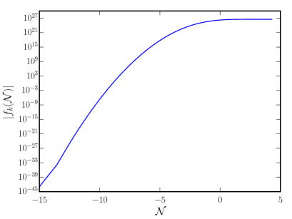
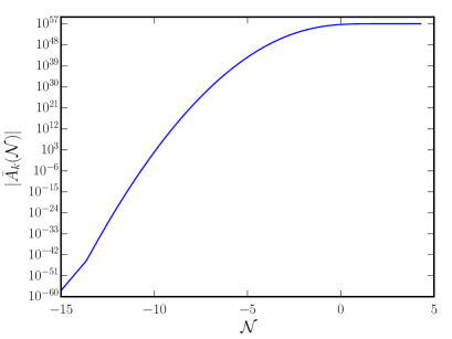
The behavior of the mode is plotted in Fig. 1 as a function of so-called e-N-folds in terms of which the scale factor is given by [64], where is the value of the scale factor at the bounce. Note that the modes and grow strongly as one approaches the bounce. Such a growth may lead to large non-Gaussianities in the bouncing scenarios.
3.2.1 The case of
Let us first consider the case of , as we had done in the context of inflation. In such a case, we have
| (3.27) |
Since we now know the background quantities as well as the behavior of the modes, we have all the information required to evaluate the integrals characterizing the three-point function [cf. Eqs. (3.11)]. In order to calculate these integrals, evidently, we can divide the period of interest (i.e. ) into two domains ( and ) over which we have constructed solutions for the modes.
In the first domain, for the bouncing scenario of our interest, the scale factor can be approximately written as . Therefore, we have [cf. Eqs. (2.21) and (3.22)]
| (3.28) |
where we have set . Also, when , the electromagnetic modes (2.22) and their time derivative reduce to
| (3.29a) | |||||
| (3.29b) | |||||
Now, in order to arrive at the three-point function, we need to evaluate the integrals (3.11). After writing these equations in terms of the coupling function and the scalar and electromagnetic modes, we find that the integrals involved are mainly of the following form:
| (3.30) |
which can be evaluated to be [85]
| (3.31a) | |||||
| (3.31b) | |||||
with being the exponential integral function. Therefore, in the first domain, the integrals (3.11) can be completely written in terms of the quantities (see Appendix for the complete expressions).
In the second domain, we have
| (3.32) |
where we have defined . Also, the modes and their derivatives are given by the expressions [cf. Eq. (2.4)]
| (3.33a) | |||||
| (3.33b) | |||||
where
| (3.34a) | |||||
| (3.34b) | |||||
with and being obtained from the corresponding values evaluated at the end of the first domain [cf. Eqs. (3.29)], while is given by Eq. (3.26). On using the above expressions, we find that the integrals (3.11) in the second domain are of the following form:
| (3.35a) | |||||
| (3.35b) | |||||
These integrals can be evaluated easily in terms of elementary functions. Thereafter, these two integrals can be combined to arrive at the total contribution to the three-point function from the second domain.
3.2.2 The case of
For the case of and , which is when scale invariant magnetic fields are generated, we have
| (3.36) |
In the first domain, for the matter bounce scenario, we therefore have
| (3.37) |
where we have set . In this case, the electromagnetic modes (2.22) in the first domain simplify to
| (3.38a) | |||||
| (3.38b) | |||||
Using these solutions, we can compute the contribution to the three-point function from the first domain. We find that the integrals (3.11) can be completely expressed in terms of the functions we had introduced in Eqs. (3.30) and (3.31) (see Appendix).
In the second domain, we have
| (3.39) |
where we have defined . Also, the electromagnetic modes are given by the following expressions [82]:
| (3.40a) | |||||
| (3.40b) | |||||
where the quantities and can be written as
| (3.41a) | |||||
| (3.41b) | |||||
while the function is given by
| (3.42) |
Upon using the above expressions for the modes, we find that the integrals (3.11) in the second domain are of the following form:
| (3.43a) | |||||
| (3.43b) | |||||
These integrals can again be evaluated easily and expressed in terms of elementary functions and they can then be combined to arrive at the complete three-point function.
It is useful to note here that, on comparing the amplitude of the contributions to the three-point function from the first and second domains, we find that the second domain leads to a much larger contribution than that from the first domain in both the cases of and . The final expressions describing the three-point functions prove to be quite lengthy and cumbersome. Due to this reason, rather than write them down explicitly, we shall instead illustrate the behavior of the corresponding non-Gaussianity parameter as density plots in the next section.
4 Amplitude and shape of the non-Gaussianity parameter
Motivated by definitions of the non-Gaussianity parameters describing the three-point auto and cross-correlations of the scalar and tensor perturbations [86, 87], we shall now define a non-Gaussianity parameter to characterize the cross-correlation between the magnetic field and the perturbation in the scalar field. As we shall see, the parameter will prove to be a dimensionless quantity involving the ratio of the cross-correlation and the power spectra of the scalar perturbation and the magnetic field. The parameter captures the amplitude and shape of the three-point function, and we should clarify that it has a form very similar to the parameters defined earlier in this context [69, 71, 72]. In this section, we shall arrive at the expression for the non-Gaussianity parameter by following the same procedure as was used to arrive at similar parameters for the three-point functions involving the scalar and tensor perturbations [87]. With the definition at hand, we shall evaluate the parameter for the inflationary and bouncing scenarios of our interest.
The amplitude of the non-Gaussianity in the local model for the scalar three-point function is usually parameterized in terms of a parameter which, in this model, coincides with the bispectrum scaled by products of the power spectra. Here, we generalize that analogously to a non-Gaussianity parameter which we define through the following relation:
| (4.1) |
where is the Fourier mode of the actual magnetic field and indicates the Fourier mode of its Gaussian part, while, as usual, refers to Fourier mode of the perturbation in the scalar field which has already been assumed to be Gaussian. We can evaluate the three-point function of our interest, viz. , upon using the above definition of and Wick’s theorem which applies to Gaussian operators. On making use of the definition (3.9) of and inverting the resulting expression, we obtain the following expression for :
| (4.2) | |||||
In this expression, is the power spectrum of the magnetic field we have discussed earlier, while is the power spectrum of the scalar field, given by
| (4.3) |
with the right hand side to be evaluated as in the context of inflation and at in the context of the bouncing models. Due to their dual nature [84], both de Sitter inflation and matter bounce are expected to lead to scale invariant spectra for the perturbation in the scalar field. In de Sitter inflation, the spectrum is given by the well known scale invariant form
| (4.4) |
In the matter bounce, using the modes (3.24), it can be determined to be [82]
| (4.5) |
Let us first consider the amplitude and shape of the non-Gaussianity parameter for an arbitrary triangular configuration of the wavevectors , and in the context of inflation. In de Sitter inflation, for the case of , from the two contributions (3.17) to the three-point function and the power spectra (2.18) and (4.4), the parameter can be obtained to be
| (4.6) | |||||
Note that, in the squeezed limit, wherein and , we have . For the case of , the non-Gaussianity parameter can be obtained [from Eqs. (3.19), (2.18) and (4.4)] to be
| (4.7) | |||||
In the squeezed limit, we have . In the next section, we shall discuss the properties of in the squeezed limit in more detail.
For the matter bounce scenario and the two cases of and that we had considered, we can arrive at the non-Gaussianity parameter from the various expressions we had obtained earlier and the corresponding power spectra. However, as the resulting expressions are too lengthy and cumbersome, we do not explicitly write them down here. We shall plot them below and compare them with the results in inflation.
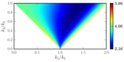
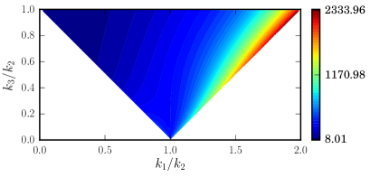
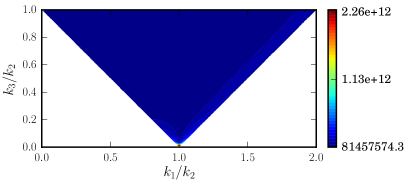
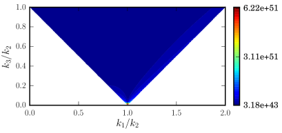
In Figs. 2 and 3, we have illustrated the non-Gaussianity parameter as a density plot for an arbitrary triangular configuration of the wavevectors , , and , as is often done for the scalar non-Gaussianity parameter (see, for instance, Ref. [86]). In these plots, the -axis corresponds to the ratio of the amplitudes of and , while the -axis corresponds to the ratio of the amplitudes of and . For the case of three-point functions involving perturbations of similar nature, such as the scalar and tensor bispectra, due to the symmetrical nature of these three-point functions, it is sufficient to construct these density plots over the domain and . However, for the cases of three-point functions involving one mode of a nature dissimilar from the other two, such as in the case of the three-point function with one scalar mode and two electromagnetic modes that we are studying here, we find that the above ranges of ratios of the wavenumbers do not adequately represent all the various combinations of wavenumbers that can arise in such a context. Therefore, in Figs. 2 and 3, we have plotted the parameter over the ranges and . These values of the ratios of wavenumbers can satisfactorily represent the entire range of triangular configuration of wavevectors of our interest.
A few points need to be stressed regarding the results that have been illustrated in Figs. 2 and 3. Let us first discuss the case of de Sitter inflation. To begin with, note that, in this case, the amplitude as well as the shape of the non-Gaussianity parameter is considerably different depending on whether or . Also, the amplitude in the case is considerably larger due to the appearance of the term, with the maximum values of the parameter arising in the flattened limit wherein . Moreover, as we already mentioned, in the squeezed limit wherein and , we have when and when . This is essentially the so-called consistency relation which we shall establish in the next section for an arbitrary in the case of inflation. In contrast, the non-Gaussianity parameter seems to have primarily the same shape for and in the matter bounce case. This can be attributed to the fact that, as the wavenumbers of cosmological interest are much smaller than the bounce scale, the matter bounce scenario is unable to strongly discriminate between these modes. However, the amplitude of in the matter bounce is considerably larger than in de Sitter inflation, which is possibly because of the form of the coupling function that we have considered. While, for , is nearly scale invariant, say, in the equilateral limit, we find that the parameter has a strong red tilt when (with behaving as ), leading to rather large values for the small wavenumbers (say, for ) corresponding to cosmological scales. We shall discuss the implications of this result in the concluding section.
5 The three-point function in the squeezed limit and the consistency relation
One of the most important characteristics of three-point functions is their behavior in the squeezed limit of the three wavenumbers, viz. when one of the three wavenumbers is much smaller than the other two, or, equivalently, when one of the three wavelengths is much longer than the other two. For the case of inflation, in this limit, the longest wavelength mode freezes on super Hubble scales and therefore acts as a background for the smaller wavelength modes. Consequently, the three-point function can be expressed in terms of the two-point functions involving the perturbations through the so-called consistency relation [75, 76]. In this section, we shall obtain the consistency relation for the three-point function involving the magnetic field and the scalar perturbation in the case of de Sitter inflation. We shall also discuss its validity in the bouncing scenario.
Let us first consider the case of de Sitter inflation. In the squeezed limit, i.e. when and, say, , the scalar mode with wavenumber can be considered to have exited the Hubble radius and hence its amplitude can be treated as a constant. Therefore, the mode can be extracted out of the integrals (3.11). For the coupling function that we had considered, given the modes (2.16), we obtain that, for arbitrary [85],
| (5.1a) | |||||
| (5.1b) | |||||
Adding the contributions due to these two integrals, the three-point function in the squeezed limit can be written as
Using this result, the expressions for the power spectra of the scalar field and the magnetic field as well as the behavior of Hankel functions for small values of , we can obtain the non-Gaussianity parameter in the squeezed limit to be [85]
| (5.3) |
where is the spectral index of the power spectrum of the magnetic field. This implies that, in the squeezed limit, for and for , results that we had already arrived at in the previous section.
In the bouncing scenario under consideration, we find that the scalar mode strongly grows as one approaches the bounce and, in fact, also exhibits a slow growth even after the bounce (in this context, see Fig. 1). Specifically, in contrast to its behavior in de Sitter inflation, the scalar mode does not become a constant at late times. Therefore, it can be expected that, contrary to the reduced integrals (5.1) that we had obtained in the squeezed limit in the inflationary context, the corresponding integrals in bounces would involve all the three modes. Consequently, the consistency relation (5.3) that is valid in the case of de Sitter inflation may not hold true in the bouncing model. On evaluating the three-point function and the non-Gaussianity parameter in the bounce, we find that the consistency relation is indeed violated. The violation of the consistency relation corresponding to the tensor bispectrum in a matter bounce was observed in a previous work [82], and it is interesting to note that a similar behavior is exhibited by the three-point function involving one scalar and two electromagnetic modes as well. This difference in the behavior of the non-Gaussianity parameter between de Sitter inflation and matter bounce scenarios, despite the similarities in the two-point functions obtained in these two models, can potentially serve as a discriminator between the inflationary paradigm and the bouncing scenarios.
6 Discussion
The magnetic fields existing on various scales in the universe are considered to have originated from a primordial seed field. Although the generation of such fields via the inflationary mechanism has been well studied, there have been far fewer endeavors to investigate the origin of the primordial magnetic fields in bouncing models. One of the most important signatures of such fields would be the extent of non-Gaussianity associated with the cross-correlations between these fields and the scalar perturbations. These three-point functions have been evaluated in certain inflationary scenarios and it has been found that the corresponding non-Gaussianity parameter can be expected to be quite large.
In the matter bounce scenario of our interest, the modes grow as one approaches the bounce, and grow very slowly thereafter. Due to the enhancement in the amplitude of the modes, it can be expected that the non-Gaussianities associated with the three-point functions would be very large. In a previous work [82], it was shown that irrespective of the growth of the tensor modes in a matter bounce, the corresponding tensor non-Gaussianities are rather small and the consistency relation for the tensor bispectrum is violated. In contrast, in this work, we find that the non-Gaussianity parameter associated with the cross-correlations involving the primordial magnetic fields and the scalar perturbations is very large and, in fact, is much larger than what is expected in the de Sitter inflationary scenario. Further, the corresponding consistency relation is violated in the bouncing model. It should be noted that the bouncing scenario that we have considered here suffers from considerable backreaction in the vicinity of the bounce [64, 65], which can possibly be responsible for the large non-Gaussianities that we encounter. This issue of circumventing the backreaction in the proximity of the bounce is non-trivial and needs to be investigated in more detail.
Recall that we have restricted ourselves to the matter bounce scenario. Evidently, other combinations of the parameters and can also lead to scale invariant magnetic power spectra of relevant amplitude. It would be interesting to examine whether other scenarios that result in similar amplitude for the scale invariant power spectrum also lead to similar results for the non-Gaussianities. Note that the extent of non-Gaussianities depends on as well as , with the latter depending on [cf. Eq. (3.22)]. Therefore, it is important to explore a wide variety of coupling functions , some of which may lead to considerably different levels of non-Gaussianities. It seems difficult to be able to make generic remarks regarding the results one can obtain from different forms of couplings. Therefore, one may have to examine the effects of each type of coupling separately. We believe that it may be challenging to simultaneously produce magnetic fields of observable strengths in bounces while also ensuring that the levels of non-Gaussianities remain as small as encountered in inflation. We are curently systematically exploring these issues.
Acknowledgements
This work was initiated during visits by DC and LS to the Department of Physics and Astronomy, Johns Hopkins University, Baltimore, Maryland, U.S.A. under the aegis of The Indo-US Science and Technology Forum grant IUSSTF/JC-Fundamental Tests of Cosmology/2-2014/2015-16. DC would like to thank the Indian Institute of Technology Madras, Chennai, India, for financial support through half-time research assistantship. LS also wishes to thank the Indian Institute of Technology Madras, Chennai, India, for support through the Exploratory Research Project PHY/17-18/874/RFER/LSRI. This work was supported at Johns Hopkins University by NSF Grant No. 1519353, NASA NNX17AK38G, and the Simons Foundation. We wish to thank Rajeev Jain for comments on the manuscript.
Appendix A Appendix: Evaluation of integrals
In this appendix, we shall provide the results for the integrals and [cf. Eqs. (3.11)] evaluated in de Sitter inflation and in the first domain in the matter bounce scenario of our interest.
Let us first consider the case in de Sitter inflation. In this case, we find that the integrals can be evaluated to be
| (A.1a) | |||||
In the case of , we find that the integrals are given by
| (A.2a) | |||||
It should be mentioned that the integrals have been regulated (as is usually done in this context) in the limit to arrive at the above results.
Let us now turn to the case of the bouncing scenario. In the first domain, as in the inflationary case, the integrals have to be suitably regulated in the first domain (in the limit) to arrive at the required results. The integrals in the second domain do not entail considering any non-trivial limits and can be evaluated in a straightforward manner. Moreover, the results for the integrals in the second domain prove to be rather lengthy. Therefore, in what follows, we shall provide the results only in the first domain.
In the case, we find that the integrals are given by
| (A.3a) | |||||
| (A.3b) | |||||
While, in the case, they can be obtained to be
References
- [1] D. Grasso and H. R. Rubinstein, Magnetic fields in the early universe, Phys. Rept. 348 (2001) 163–266, [astro-ph/0009061].
- [2] L. M. Widrow, Origin of Galactic and Extragalactic Magnetic Fields, Rev. Mod. Phys. 74 (2002) 775–823, [astro-ph/0207240].
- [3] A. Kandus, K. E. Kunze, and C. G. Tsagas, Primordial magnetogenesis, Phys. Rept. 505 (2011) 1–58, [arXiv:1007.3891].
- [4] L. M. Widrow, D. Ryu, D. R. Schleicher, K. Subramanian, C. G. Tsagas, et al., The First Magnetic Fields, Space Sci. Rev. 166 (2012) 37–70, [arXiv:1109.4052].
- [5] R. Durrer and A. Neronov, Cosmological Magnetic Fields: Their Generation, Evolution and Observation, Astron. Astrophys. Rev. 21 (2013) 62, [arXiv:1303.7121].
- [6] K. Subramanian, The origin, evolution and signatures of primordial magnetic fields, Rept. Prog. Phys. 79 (2016), no. 7 076901, [arXiv:1504.02311].
- [7] A. Neronov and I. Vovk, Evidence for strong extragalactic magnetic fields from Fermi observations of TeV blazars, Science 328 (2010) 73–75, [arXiv:1006.3504].
- [8] F. Tavecchio et al., The intergalactic magnetic field constrained by Fermi/LAT observations of the TeV blazar 1ES 0229+200, Mon. Not. Roy. Astron. Soc. 406 (2010) L70–L74, [arXiv:1004.1329].
- [9] C. D. Dermer, M. Cavadini, S. Razzaque, J. D. Finke, and B. Lott, Time Delay of Cascade Radiation for TeV Blazars and the Measurement of the Intergalactic Magnetic Field, Astrophys. J. 733 (2011) L21, [arXiv:1011.6660].
- [10] I. Vovk, A. M. Taylor, D. Semikoz, and A. Neronov, Fermi/LAT observations of 1ES 0229+200: implications for extragalactic magnetic fields and background light, Astrophys. J. 747 (2012) L14, [arXiv:1112.2534].
- [11] F. Tavecchio, G. Ghisellini, G. Bonnoli, and L. Foschini, Extreme TeV blazars and the intergalactic magnetic field, Mon. Not. Roy. Astron. Soc. 414 (2011) 3566, [arXiv:1009.1048].
- [12] K. Dolag, M. Kachelriess, S. Ostapchenko, and R. Tomas, Lower limit on the strength and filling factor of extragalactic magnetic fields, Astrophys. J. 727 (2011) L4, [arXiv:1009.1782].
- [13] A. M. Taylor, I. Vovk, and A. Neronov, Extragalactic magnetic fields constraints from simultaneous GeV-TeV observations of blazars, Astron. Astrophys. 529 (2011) A144, [arXiv:1101.0932].
- [14] K. Takahashi, M. Mori, K. Ichiki, and S. Inoue, Lower Bounds on Intergalactic Magnetic Fields from Simultaneously Observed GeV-TeV Light Curves of the Blazar Mrk 501, Astrophys. J. 744 (2012) L7, [arXiv:1103.3835].
- [15] H. Huan, T. Weisgarber, T. Arlen, and S. P. Wakely, A New Model for Gamma-Ray Cascades in Extragalactic Magnetic Fields, Astrophys. J. 735 (2011) L28, [arXiv:1106.1218].
- [16] J. D. Finke, L. C. Reyes, M. Georganopoulos, K. Reynolds, M. Ajello, S. J. Fegan, and K. McCann, Constraints on the Intergalactic Magnetic Field with Gamma-Ray Observations of Blazars, Astrophys. J. 814 (2015), no. 1 20, [arXiv:1510.02485].
- [17] Planck Collaboration, P. Ade et al., Planck 2015 results. XIX. Constraints on primordial magnetic fields, arXiv:1502.01594.
- [18] POLARBEAR Collaboration, P. A. R. Ade et al., POLARBEAR Constraints on Cosmic Birefringence and Primordial Magnetic Fields, Phys. Rev. D92 (2015) 123509, [arXiv:1509.02461].
- [19] M. S. Pshirkov, P. G. Tinyakov, and F. R. Urban, New limits on extragalactic magnetic fields from rotation measures, Phys. Rev. Lett. 116 (2016), no. 19 191302, [arXiv:1504.06546].
- [20] B. Ratra, Cosmological ’seed’ magnetic field from inflation, Astrophys. J. 391 (1992) L1–L4.
- [21] K. Bamba and J. Yokoyama, Large scale magnetic fields from inflation in dilaton electromagnetism, Phys. Rev. D69 (2004) 043507, [astro-ph/0310824].
- [22] K. Bamba and M. Sasaki, Large-scale magnetic fields in the inflationary universe, JCAP 0702 (2007) 030, [astro-ph/0611701].
- [23] V. Demozzi, V. Mukhanov, and H. Rubinstein, Magnetic fields from inflation?, JCAP 0908 (2009) 025, [arXiv:0907.1030].
- [24] J. Martin and J. Yokoyama, Generation of Large-Scale Magnetic Fields in Single-Field Inflation, JCAP 0801 (2008) 025, [arXiv:0711.4307].
- [25] L. Campanelli, Helical Magnetic Fields from Inflation, Int. J. Mod. Phys. D18 (2009) 1395–1411, [arXiv:0805.0575].
- [26] S. Kanno, J. Soda, and M.-a. Watanabe, Cosmological Magnetic Fields from Inflation and Backreaction, JCAP 0912 (2009) 009, [arXiv:0908.3509].
- [27] K. Subramanian, Magnetic fields in the early universe, Astron. Nachr. 331 (2010) 110–120, [arXiv:0911.4771].
- [28] F. R. Urban, On inflating magnetic fields, and the backreactions thereof, JCAP 1112 (2011) 012, [arXiv:1111.1006].
- [29] R. Durrer, L. Hollenstein, and R. K. Jain, Can slow roll inflation induce relevant helical magnetic fields?, JCAP 1103 (2011) 037, [arXiv:1005.5322].
- [30] C. T. Byrnes, L. Hollenstein, R. K. Jain, and F. R. Urban, Resonant magnetic fields from inflation, JCAP 1203 (2012) 009, [arXiv:1111.2030].
- [31] R. K. Jain, R. Durrer, and L. Hollenstein, Generation of helical magnetic fields from inflation, J.Phys.Conf.Ser. 484 (2014) 012062, [arXiv:1204.2409].
- [32] T. Kahniashvili, A. Brandenburg, L. Campanelli, B. Ratra, and A. G. Tevzadze, Evolution of inflation-generated magnetic field through phase transitions, Phys.Rev. D86 (2012) 103005, [arXiv:1206.2428].
- [33] S.-L. Cheng, W. Lee, and K.-W. Ng, Inflationary dilaton-axion magnetogenesis, arXiv:1409.2656.
- [34] K. Bamba, Generation of large-scale magnetic fields, non-Gaussianity, and primordial gravitational waves in inflationary cosmology, Phys. Rev. D91 (2015) 043509, [arXiv:1411.4335].
- [35] T. Fujita, R. Namba, Y. Tada, N. Takeda, and H. Tashiro, Consistent generation of magnetic fields in axion inflation models, JCAP 1505 (2015), no. 05 054, [arXiv:1503.05802].
- [36] L. Campanelli, Lorentz-violating inflationary magnetogenesis, Eur. Phys. J. C75 (2015), no. 6 278, [arXiv:1503.07415].
- [37] T. Fujita and R. Namba, Pre-reheating Magnetogenesis in the Kinetic Coupling Model, arXiv:1602.05673.
- [38] C. G. Tsagas, Causality, initial conditions, and inflationary magnetogenesis, Phys. Rev. D93 (2016), no. 10 103529, [arXiv:1603.05209].
- [39] R. J. Ferreira, R. K. Jain, and M. S. Sloth, Inflationary magnetogenesis without the strong coupling problem, JCAP 1310 (2013) 004, [arXiv:1305.7151].
- [40] R. J. Ferreira, R. K. Jain, and M. S. Sloth, Inflationary Magnetogenesis without the Strong Coupling Problem II: Constraints from CMB anisotropies and B-modes, JCAP 1406 (2014) 053, [arXiv:1403.5516].
- [41] F. Finelli and R. Brandenberger, On the generation of a scale invariant spectrum of adiabatic fluctuations in cosmological models with a contracting phase, Phys.Rev. D65 (2002) 103522, [hep-th/0112249].
- [42] J. Martin, P. Peter, N. Pinto Neto, and D. J. Schwarz, Passing through the bounce in the ekpyrotic models, Phys.Rev. D65 (2002) 123513, [hep-th/0112128].
- [43] S. Tsujikawa, R. Brandenberger, and F. Finelli, On the construction of nonsingular pre - big bang and ekpyrotic cosmologies and the resulting density perturbations, Phys.Rev. D66 (2002) 083513, [hep-th/0207228].
- [44] P. Peter and N. Pinto-Neto, Primordial perturbations in a non singular bouncing universe model, Phys.Rev. D66 (2002) 063509, [hep-th/0203013].
- [45] J. Martin and P. Peter, Parametric amplification of metric fluctuations through a bouncing phase, Phys.Rev. D68 (2003) 103517, [hep-th/0307077].
- [46] J. Martin and P. Peter, On the causality argument in bouncing cosmologies, Phys.Rev.Lett. 92 (2004) 061301, [astro-ph/0312488].
- [47] P. Peter, N. Pinto-Neto, and D. A. Gonzalez, Adiabatic and entropy perturbations propagation in a bouncing universe, JCAP 0312 (2003) 003, [hep-th/0306005].
- [48] J. Martin and P. Peter, On the properties of the transition matrix in bouncing cosmologies, Phys.Rev. D69 (2004) 107301, [hep-th/0403173].
- [49] L. E. Allen and D. Wands, Cosmological perturbations through a simple bounce, Phys.Rev. D70 (2004) 063515, [astro-ph/0404441].
- [50] T. Battefeld, S. P. Patil, and R. Brandenberger, Non-singular perturbations in a bouncing brane model, Phys.Rev. D70 (2004) 066006, [hep-th/0401010].
- [51] P. Creminelli, A. Nicolis, and M. Zaldarriaga, Perturbations in bouncing cosmologies: Dynamical attractor versus scale invariance, Phys.Rev. D71 (2005) 063505, [hep-th/0411270].
- [52] G. Geshnizjani, T. J. Battefeld, and G. Geshnizjani, A Note on perturbations during a regular bounce, Phys.Rev. D73 (2006) 048501, [hep-th/0506139].
- [53] L. R. Abramo and P. Peter, K-Bounce, JCAP 0709 (2007) 001, [arXiv:0705.2893].
- [54] P. Peter and N. Pinto-Neto, Cosmology without inflation, Phys.Rev. D78 (2008) 063506, [arXiv:0809.2022].
- [55] F. T. Falciano, M. Lilley, and P. Peter, A Classical bounce: Constraints and consequences, Phys.Rev. D77 (2008) 083513, [arXiv:0802.1196].
- [56] A. Cardoso and D. Wands, Generalised perturbation equations in bouncing cosmologies, Phys.Rev. D77 (2008) 123538, [arXiv:0801.1667].
- [57] M. Novello and S. P. Bergliaffa, Bouncing Cosmologies, Phys.Rept. 463 (2008) 127–213, [arXiv:0802.1634].
- [58] J.-L. Lehners, Ekpyrotic and Cyclic Cosmology, Phys. Rept. 465 (2008) 223–263, [arXiv:0806.1245].
- [59] D. Battefeld and P. Peter, A Critical Review of Classical Bouncing Cosmologies, Phys.Rept. 571 (2015) 1–66, [arXiv:1406.2790].
- [60] R. Brandenberger and P. Peter, Bouncing Cosmologies: Progress and Problems, arXiv:1603.05834.
- [61] Y.-F. Cai, Exploring Bouncing Cosmologies with Cosmological Surveys, Sci. China Phys. Mech. Astron. 57 (2014) 1414–1430, [arXiv:1405.1369].
- [62] J. Salim, N. Souza, S. E. Perez Bergliaffa, and T. Prokopec, Creation of cosmological magnetic fields in a bouncing cosmology, JCAP 0704 (2007) 011, [astro-ph/0612281].
- [63] F. A. Membiela, Primordial magnetic fields from a non-singular bouncing cosmology, Nucl.Phys. B885 (2014) 196–224, [arXiv:1312.2162].
- [64] L. Sriramkumar, K. Atmjeet, and R. K. Jain, Generation of scale invariant magnetic fields in bouncing universes, JCAP 1509 (2015), no. 09 010, [arXiv:1504.06853].
- [65] D. Chowdhury, L. Sriramkumar, and R. K. Jain, Duality and scale invariant magnetic fields from bouncing universes, Phys. Rev. D94 (2016), no. 8 083512, [arXiv:1604.02143].
- [66] I. Ben-Dayan, Gravitational Waves in Bouncing Cosmologies from Gauge Field Production, JCAP 1609 (2016), no. 09 017, [arXiv:1604.07899].
- [67] R. Koley and S. Samtani, Magnetogenesis in Matter - Ekpyrotic Bouncing Cosmology, JCAP 1704 (2017), no. 04 030, [arXiv:1612.08556].
- [68] A. Ito and J. Soda, Primordial Gravitational Waves Induced by Magnetic Fields in an Ekpyrotic Scenario, Phys. Lett. B771 (2017) 415–420, [arXiv:1607.07062].
- [69] R. R. Caldwell, L. Motta, and M. Kamionkowski, Correlation of inflation-produced magnetic fields with scalar fluctuations, Phys. Rev. D84 (2011) 123525, [arXiv:1109.4415].
- [70] L. Motta and R. R. Caldwell, Non-Gaussian features of primordial magnetic fields in power-law inflation, Phys. Rev. D85 (2012) 103532, [arXiv:1203.1033].
- [71] R. K. Jain and M. S. Sloth, Consistency relation for cosmic magnetic fields, Phys. Rev. D86 (2012) 123528, [arXiv:1207.4187].
- [72] R. K. Jain and M. S. Sloth, On the non-Gaussian correlation of the primordial curvature perturbation with vector fields, JCAP 1302 (2013) 003, [arXiv:1210.3461].
- [73] K. E. Kunze, CMB and matter power spectra from cross correlations of primordial curvature and magnetic fields, Phys. Rev. D87 (2013), no. 10 103005, [arXiv:1301.6105].
- [74] R. N. Raveendran, D. Chowdhury, and L. Sriramkumar, Viable tensor-to-scalar ratio in a symmetric matter bounce, JCAP 1801 (2018), no. 01 030, [arXiv:1703.10061].
- [75] J. M. Maldacena, Non-Gaussian features of primordial fluctuations in single field inflationary models, JHEP 05 (2003) 013, [astro-ph/0210603].
- [76] P. Creminelli and M. Zaldarriaga, Single field consistency relation for the 3-point function, JCAP 0410 (2004) 006, [astro-ph/0407059].
- [77] S. Kundu, Non-Gaussianity Consistency Relations, Initial States and Back-reaction, JCAP 1404 (2014) 016, [arXiv:1311.1575].
- [78] V. Sreenath and L. Sriramkumar, Examining the consistency relations describing the three-point functions involving tensors, JCAP 1410 (2014), no. 10 021, [arXiv:1406.1609].
- [79] V. Sreenath, D. K. Hazra, and L. Sriramkumar, On the scalar consistency relation away from slow roll, JCAP 1502 (2015), no. 02 029, [arXiv:1410.0252].
- [80] E. Dimastrogiovanni, M. Fasiello, D. Jeong, and M. Kamionkowski, Inflationary tensor fossils in large-scale structure, JCAP 1412 (2014) 050, [arXiv:1407.8204].
- [81] E. Dimastrogiovanni, M. Fasiello, and M. Kamionkowski, Imprints of Massive Primordial Fields on Large-Scale Structure, JCAP 1602 (2016) 017, [arXiv:1504.05993].
- [82] D. Chowdhury, V. Sreenath, and L. Sriramkumar, The tensor bi-spectrum in a matter bounce, JCAP 1511 (2015) 002, [arXiv:1506.06475].
- [83] Wolfram Research, Inc., Mathematica, Version 11.0. Champaign, IL, 2016.
- [84] D. Wands, Duality invariance of cosmological perturbation spectra, Phys. Rev. D60 (1999) 023507, [gr-qc/9809062].
- [85] I. S. Gradshteyn and I. M. Ryzhik, Table of Integrals, Series, and Products. Academic Press, New York, 7th ed., 2007.
- [86] E. Komatsu, Hunting for Primordial Non-Gaussianity in the Cosmic Microwave Background, Class. Quant. Grav. 27 (2010) 124010, [arXiv:1003.6097].
- [87] V. Sreenath, R. Tibrewala, and L. Sriramkumar, Numerical evaluation of the three-point scalar-tensor cross-correlations and the tensor bi-spectrum, JCAP 1312 (2013) 037, [arXiv:1309.7169].