Learning Probabilistic Logic Programs in Continuous Domains

Abstract

The field of statistical relational learning aims at unifying logic and probability to reason and learn from data. Perhaps the most successful paradigm in the field is probabilistic logic programming: the enabling of stochastic primitives in logic programming, which is now increasingly seen to provide a declarative background to complex machine learning applications. While many systems offer inference capabilities, the more significant challenge is that of learning meaningful and interpretable symbolic representations from data. In that regard, inductive logic programming and related techniques have paved much of the way for the last few decades.

Unfortunately, a major limitation of this exciting landscape is that much of the work is limited to finite-domain discrete probability distributions. Recently, a handful of systems have been extended to represent and perform inference with continuous distributions. The problem, of course, is that classical solutions for inference are either restricted to well-known parametric families (e.g., Gaussians) or resort to sampling strategies that provide correct answers only in the limit. When it comes to learning, moreover, inducing representations remains entirely open, other than “data-fitting” solutions that force-fit points to aforementioned parametric families.

In this paper, we take the first steps towards inducing probabilistic logic programs for continuous and mixed discrete-continuous data, without being pigeon-holed to a fixed set of distribution families. Our key insight is to leverage techniques from piecewise polynomial function approximation theory, yielding a principled way to learn and compositionally construct density functions. We test the framework and discuss the learned representations.

Introduction

The field of statistical relational learning aims at unifying logic and probability to reason and learn from relational data. Logic provides a means to codify high-level dependencies between individuals, enabling descriptive clarity in the knowledge representation system. Perhaps the most successful paradigm in the field is probabilistic logic programming (PLP): the enabling of stochastic primitives in logic programming. Programmatic abstractions further enable modularity and compositionality, and are now increasingly seen as providing a much needed declarative interface for complex machine learning applications (?).

While a great deal of attention has been paid to the semantics and inference computations of such programming languages (?; ?; ?), it is the learning of representations that is deeply challenging. Parameter learning attempts to obtain the probabilities of atoms from observational traces (e.g., number of heads observed in a sequence of coin tosses) (?; ?). The significantly harder problem is that of structure learning: for example, learning (deterministic) rules – essentially, logic programs – from data. The influential work on inductive logic programming and first-order rule learning (?; ?) is a major step in this direction. Viewed from the perspective of program synthesis (?), it is worthwhile to remark that the learning objectives, the synthesis process and the final outcome are all expressed in the same language (?). Rule learning is now widely used in natural language processing (NLP) applications for Web data (?), among others. Naturally, the hardest variant here is to additionally learn probabilistic atoms together with these rules (e.g., (?)), so as to yield a probabilistic logic program. This is done by first learning deterministic rules, and then the weights are determined in a second step using parameter estimation techniques.

Unfortunately, a major limitation of this exciting landscape is that much of the work is limited to finite-domain discrete probability distributions. This is a very serious limitation because for many forms of data – including time-series data, such as temperature observations, trajectories of moving objects, and financial data – continuous representations are the most natural and compact. Disciplines from robotics to social sciences and biology formulate their findings using continuous, and mixed discrete-continuous probability distributions. Admittedly, there has been some effort in representing and inferring with continuous distributions in a logic programming context (e.g., (?; ?; ?)).

But inference is difficult; it requires one to either restrict to well-known parametric families (e.g., Gaussians) for efficiency or choose proposal distributions carefully, and then resort to sampling strategies that provide correct answers only in the limit. When it comes to learning, however, inducing representations remains almost entirely open. Conventional “data-fitting” solutions, for example, force-fit points to parametric families (?). In fact, to the best of our knowledge, the only approach that discusses the learning of probabilistic logic programs in continuous settings is that of (?), but this assumes that base distributions (i.e., probabilistic atoms) are Gaussian, and then develops a decision-tree learner for inducing rules from observational traces of these atoms.

In this paper, we take steps to fill this gap. We make three key contributions. First, we address the problem of learning continuous probabilistic atoms but without being pigeon-holed to a fixed set of distribution families; indeed, the shape of the underlying distribution can be arbitrarily complex by appealing to piecewise polynomial approximations (?). Efficient integration is possible for that representation (?). Second, (discrete) predicates denoting the pieces from that base distribution are then used to learn deterministic rules, yielding dependencies between sub-spaces of a mixed discrete-continuous probability space. What is particularly attractive about this strategy is that the rule learning can be performed using any standard discrete learner. Third, by interfacing a symbolic integration algorithm with a discrete PLP system, we obtain a modular approach for inferring with PLPs in continuous domains. While much of the underlying machinery is agnostic about the PLP language, we develop and implement our approach on ProbLog and its continuous extension (?) for the sake of concreteness. In a subsequent section, we report on empirical evaluations and discuss the learned representations. To the best of our knowledge, this is the first attempt to induce probabilistic logic programs over continuous features without making any assumptions about the underlying true density, and we hope it will make probabilistic knowledge representation systems more applicable for big uncertain data.

Related Work

Inference and learning in probabilistic systems are fundamental problems within AI, to which our work here contributes. We begin by remarking that there is an important distinction to be made between relational graphical models (?) and the inductive logic programming machinery that we use here (?). A comprehensive discussion on the subtleties would be out of scope, and orthogonal to the main thrust of the paper.

The majority of the literature focuses on inference and learning with discrete random variables, e.g., (?; ?).

Nonetheless, learning relational features from data is very popular in NLP and related areas (?; ?). Rule learning has been studied in many forms, e.g., (?; ?).

Approaches such as (?) have further applied rule learning to complex applications such as automated planning.

Treating continuous and hybrid data in such contexts, however, is rare. Part of the problem is that inference in mixed discrete-continuous distributions is already very challenging, and learning typically makes use of inference computations to guess good models. Existing inference schemes for hybrid data are either approximate, e.g., (?), or make restrictive assumptions about the distribution family (e.g., Gaussian potentials (?)). Structure learning schemes, consequently, inherit these limitations, e.g., (?).

In the PLP community, (?) discussed above, learn rules by assuming Gaussian base atoms.

The restrictive nature of parametric families has led to intense activity on piecewise polynomial constructions, e.g., (?; ?; ?). On the one hand, this representation is general, in that it can be made arbitrarily close to non-polynomial density functions (such as normal and log-normal), by increasing the degree of polynomials and the granularity of the piecewise composition (e.g., (?; ?)). On the other, under mild conditions, it supports efficient integration (e.g., (?; ?)). Recently, weighted model integration (WMI) was proposed as a computational abstraction for computing probabilities with continuous and mixed discrete-continuous distributions (?; ?; ?) based on piecewise polynomials. It generalises weighted model counting that is defined over propositional formulas for finite-domain discrete probability distributions, which is the backbone of ProbLog’s inference engine (?).

Preliminaries

Logic Programming

First, we recall the basics of Prolog and logic programming. A term $t$ denotes either a constant, a variable or a functor.

An atom $p(t_{1},..,t_{n})$ is obtained by applying terms $t_{1},\ldots,t_{n}$ to the $n$-ary relation $p$.

An atom is called ground if all its terms are constants.

A literal denotes an atom or its negation. A clause is a disjunction of literals.

If a clause only contains one non-negated atom, the clause is called definite. Such clauses are written $h\leftarrow b_{1},...,b_{n}$, where $h$ is the called the head, and the rest the body, all of which are atoms. A Prolog program is a set of definite clauses.

Variables $V_{i}$ are mapped to terms $t_{i}$ through substitution:

$$\theta=\{V_{1}/t_{1},...,V_{n}/t_{n}\}$$

A grounding substitution for an atom $a\theta$ maps all its logical variables to constants.

ProbLog

ProbLog is a probabilistic extension of Prolog (?). In addition to the set of definite clauses $D$, described above, it allows the specification of probabilistic facts, background knowledge and evidence. Facts $c_{i}$ are given probabilities $p_{i}$ to build a set of probabilistic facts that form the basis of ProbLog programs: $T=\{p_{1}::c_{1},\ldots,p_{n}::c_{n}\}$. The probabilities model how likely it is that a grounding instance $c_{i}\theta$ is true. Given a set $L_{T}=\{c_{1}\theta_{1},\ldots,c_{n}\theta_{m}\}$ of such instances ProbLog defines a probability distribution over subsets of facts $L\subseteq L_{T}$ as:

$$P(L\mid T)=\prod_{c_{i}\theta_{j}\in L}p_{i}\prod_{c_{i}\theta_{j}\in L_{T}\setminus L}(1-p_{i})$$

The success probability of a query $q$ is then defined as:

$$P_{s}(q\mid T)=\sum_{L\subseteq L_{T}\colon L\cup D\models q}P(L|T)$$

Exact inference for a ProbLog program is performed by converting the program space $L$ to a set of weighted Boolean formulas $\phi$, and computing the sum of the weights of interpretations (?).

ProbFOIL

Structure learning was recently discussed using the approach of ProbFOIL, a probabilistic extension of classical FOIL learners (?). It even allows for noisy examples. The problem is defined as:

Definition 1

(?) Given:

1. A set of examples $E$, consisting of pairs $(x_{i},p_{i})$ where $x_{i}$ is a ground fact for the unknown target predicate t and $p_{i}$ is the target probability.

2. A background theory $B$ containing information about the examples in the form of a ProbLog program;

3. A loss function $\mbox{loss}(H,B,E)$, measuring the loss of a hypothesis (set of clauses) $H$ w.r.t $B$ and $E$;

4. A space of possible clauses $L_{h}$ specified using a declarative bias;

Find: A hypothesis $H\subseteq L_{H}$ such that $H=\mbox{arg min\_H}\quad loss(H,B,E)$.

(We omit the definition of the loss function.) For simplicity, in this paper, we use ProbFOIL in a deterministic/noise-free setting (i.e., $p_{i}=1$).

Hybrid ProbLog

Hybrid ProbLog (?) extends ProbLog to support continuous densities in parametric form, such as Gaussians. In addition to the set of probabilistic facts, hybrid ProbLog consists of probabilistic continuous facts:

$$F^{c}=\{(X_{1},\phi_{1})::f_{1}^{c},...(X_{m},\phi_{m})::f_{m}^{c}\}$$

Here, $X_{i}$ a Prolog variable that is bound to a (say) Gaussian density $\phi_{i}$ that belongs to the atom $f_{i}^{c}$. For example,

(I,Gaussian(90,10)) :: intelligence(I). says that the intelligence (of, say, students in some class) modelled as a numeric value (such as IQ) is normally distributed around a mean value of 90 and standard deviation 10. Analogously, a Gaussian mixture model can be expressed using:

0.6 :: heads.(I,Gaussian(110,10)) :: intelligence_smart(I).mix(I) :- heads, intelligence(I).mix(I) :- intelligence_smart(I), \+ heads. In order to perform inference and query in this language, 3 predicates are additionally introduced: (?):

• below$(X,c)$: succeeds if X can be grounded to a continuous value and $X<c$ for the constant c.

• above$(X,c)$: succeeds if X can be grounded to a continuous value and $X>c$ for the constant c.

• ininterval$(X,c_{1},c_{2})$ succeeds if X can be grounded to a continuous value and $c_{1}\leq X\leq c_{2}$ for two constants $c_{1},c_{2}$.

Queries are build by binding a continuous relation to an interval. For example:

average :- intelligence(I), ininterval(I,65,85). says that average is true if the intelligence measure is between 65 and 85. Naturally, given the above distribution, one could ask:

query(average). This would return the probability for the interval $[65,85]$ as determined by the Gaussian above.

In general, the success probability of query is an adaptation of the discrete case and takes the form:

$$P_{s}(q\mid T)=\sum_{L\subseteq L_{T}}\sum_{I\in A\colon L\cup L_{I}\cup D\models q}P(L\mid T)\cdot\delta.$$

The intuition here is this. The query $q$ clearly determines a subspace of the domain of a random variable (i.e., $[65,85]$), and so imagine $A$ to partition $[-\infty,\infty]$ to intervals, one of which contains $q$. Thus, the success probability is defined by summing over the elements of this partition (e.g., $<65$, $q$ and $>85$), with the understanding that $L_{I}$ expresses this interval (by relativising w.r.t. $\tt above,below,ininterval$). For each such interval, we compute the success of $q$ w.r.t. the product of density functions $\delta.$ In practice, the algorithm for computing these probabilities proceeds by realising such a partition, computing integrals for the intervals and then essentially reverting to the discrete program space (?).

Framework

The aim of our framework is to provide a principled unsupervised way to learn hybrid (PLP) programs from data and to support exact inference over univariate as well as multivariate densities.

For this, to avoid being pigeon-holed to a fixed set of distributions, we appeal to piecewise polynomials that approximate any density arbitrarily close. (Cf. discussion on piecewise polynomial density approximations). Furthermore, we show how to learn the optimal underlying piecewise structure and how to leverage that piecewise structure to learn rules to yield a granular hybrid program. An example of a good and a bad approximation can be found in Figure 1.

While much of the underlying learning machinery is agnostic about the PLP language, we develop our framework on ProbLog for the sake of concreteness.

Mainly, we utilise and extend the syntax of Hybrid ProbLog and show how to use ProbLog’s discrete rule learner ProbFOIL to learn hybrid programs. We reiterate that this is an important feature.

While some prior accounts have taken steps towards extending a language to continuous domains (w.r.t. restricted, often parametric, families), none show how a standard discrete structure learner suffices. The ability to learn arbitrary PDFs together with effective inference (?) makes the framework, in our view, novel and powerful.

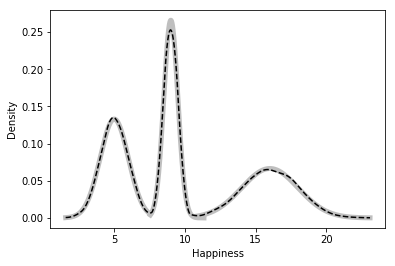
(a) Approximation 12 intervals

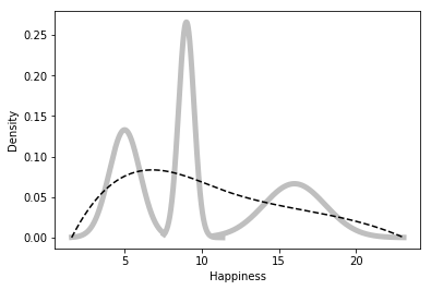
(b) Approximation 2 intervals

Figure 1: The fictional happiness attribute

Inference with Piecewise Polynomials

This section discusses our first contribution. To prepare for the learning of arbitrary PDFs, we need to revisit hybrid ProbLog. As discussed, we propose to model density functions as piecewise polynomials (PP). On the one hand, piecewise polynomial representations can be made arbitrarily close to any distribution (?). On the other hand, these representations are amenable to effective integration (?), scaling to hundreds of variables, e.g., (?). Our first contribution discusses how to: (a) model PP densities in Hybrid ProbLog with a slightly revised syntax, but without affecting the semantic devices; and (b) leverage symbolic integration techniques to compute success probabilities.

Let us begin with the syntax, and expected behaviour of queries.

Definition 2

A piecewise function over a real-valued variable $x$ is defined over $l$ pieces as:

$$\vec{pp}(X)=\begin{cases}0&x<\textit{cp}_{0}\\ {pp}_{1}(x)&\textit{cp}_{0}\leq x\leq\textit{cp}_{1}\\ ...\\ {pp}_{l}(x)&\textit{cp}_{l_{1}}\leq x\leq\textit{cp}_{l}\\ 0&x>\textit{cp}_{l}\end{cases}$$

where the intervals (expressed using cutpoints) are mutually exclusive, and each ${pp}_{i}(x)$ is a polynomial with the same maximum polynomial order $k$ of the form:

$${pp}_{i}(x)=b_{0}^{i}+b_{1}^{i}*x+...+b_{k}^{i}*x^{k}.$$

In order for $\vec{pp}(x)$ to form a valid density, $\sum_{i=1}^{l}\int_{{cp}_{i-1}}^{{cp}_{i}}{pp}_{i}(x)dx=1$.

Figure 1 demonstrates the importance of choosing the right parameters for each interval in order to approximate the function well.

When it comes to the program itself, then, for every continuous random variable, a new relation is added corresponding to each piece, defined using the original continuous attribute and further relativisation using the predicates above, below and ininterval. For example, reconsider the intelligence random variable from above, and suppose we would like to approximate the Gaussian using a 5-piece piecewise polynomial density function.

The program might include sentences such as:

-0.024719432823743857 + 0.0005171566890546171 I  :: int_low(I).int_low(I) :- intelligence(I), below(I,70).int_mid(I) :- intelligence(I), ininterval(I,70,90). What is particularly interesting about this reformulated program is that the partitioning of the real space needed for computing success probabilities in Hybrid ProbLog is already in place, and moreover, syntactically it resembles standard ProbLog, except for non-numeric weights on atoms. Thus, the success probability of query can be computed externally and returned to (standard) ProbLog to be used in the evaluation of the program.

To understand how that works, suppose now, we are interested in the probability of $\tt average$ as before. The framework then splits the query into two relations by using the intervals from the program:

average1 :- intelligence(I),ininterval(I,65,70).average2 :- intelligence(I),ininterval(I,70,85).

The probability of $\tt average1$ can be computed using the PP density for $\tt int\_low(I)$ using: $\int_{65}^{70}-0.024719432823743857+0.0005171566890546171xdx$, and that of $\tt average2$ can be computed using the PP density for $\tt int\_mid(I)$ (omitted). It then follows that the success probability of $\tt average$ is the sum of $\tt average1$ and $\tt average2.$

In general, as the density is defined as a piecewise polynomial $\vec{pp}(x)$ with $l$ pieces and cutpoints $[\textit{cp}_{i-1},\textit{cp}_{i}]$, $i=1,...,l$ the total area is obtained as follows:

$$\int_{\textit{cp}_{0}}^{\textit{cp}_{1}}\textit{pp}_{1}(x)\textit{dx}+...+\int_{\textit{cp}_{l-1}}^{\textit{cp}_{l}}\textit{pp}_{l}(x)\textit{dx}$$

Note that although $x$ is a real-valued variable and so the domain is defined on $[-\infty,\infty]$, by definition it is 0 outside of $[\textit{cp}_{0},\textit{cp}_{l}]$.

Therefore, the probability of a query $x\in[a,b]$ is computed as:

$$P(x\in[a,b])=\int_{a}^{\textit{cp}_{i}}\textit{pp}_{i}(x)\textit{dx}+...+\int_{\textit{cp}_{j-1}}^{b}\textit{pp}_{j}(x)\textit{dx}.$$

Negated atoms, which are then equivalent to $x\not\in[a,b]$ are obtained by applying $P(x\not\in[a,b])=1-P(x\in[a,b])$, because the PPs specified in the program are assumed to define a valid density. (In the following section, we discuss how to learn valid probability densities.)

To reiterate, the attractiveness of this approach is that it allows us to handle continuous computations externally and return success probabilities of (final or intermediate) query atoms to (classical) ProbLog. It seems to us that such a scheme is very much in the spirit of the original Hybrid ProbLog proposal (?), but achieves a more direct path from program transformation to inference computation.

Perhaps the most serious limitation of (?) is that the computational machinery is restricted to univariate distributions: logically speaking, unary relations. We show later that this limitation does not apply to our inference engine.

Learning Weighted Atoms

This section discusses our second contribution. We present a fully unsupervised approach to jointly learn intervals and their piecewise polynomial densities from data. The goal of this learner is to divide the attribute into $l$ optimal pieces such that the PP density approximates the data well without any knowledge of the true density. This is achieved in two steps. First, the attribute is divided into $l$ pieces given a criterion. Then, the PP weights for the intervals are calculated.

How well PPs estimate the data is determined by a noise reducing scoring function – the so-called Bayesian Information Criterion (BIC) score (?) – so as to avoid overfitting. The algorithm chooses the best discretisation and PP approximation given a set of discretisation criteria, numbers of pieces and polynomial orders.

Discretisation

In our context, discretisation refers to dividing the range of a continuous variable into $l$ mutually exclusive intervals according to some criteria. Suppose $X$ is a real-valued variable – logically, think of the argument in $\tt intelligence(X)$ – and suppose $x_{min},\ldots,x_{max}$ are the data points we observe. Discretisation yields $I=\{[\textit{cp}_{0},\textit{cp}_{1}],...,[\textit{cp}_{l-1},\textit{cp}_{l}]\}$. The set of cutpoints $\textit{CP}=\{\textit{cp}_{0},...,\textit{cp}_{l}\}$ determine the interval such that $\textit{cp}_{i-1}<\textit{cp}_{i}$, $i\in\{1,...,l\}$, $\textit{cp}_{0}=x_{min}$ and $\textit{cp}_{l}=x_{max}$. The discretisation step, therefore, defines intervals over the domain $\Omega=[x_{min},x_{max}]$.

To find the best set of intervals, ideally, the whole space of possible cutpoints should be searched exhaustively.

However, as the attribute is continuous, there exist infinitely many possibilities. To restrict the search as much as possible we aim to find simple discretisation schemes that fulfil two criteria to lay the groundwork for the PP learning:

1. Cutpoints should span the entire set of data points (i.e., attribute instances). Discretisations that only focus on parts of the attribute’s values will never be able to model the distribution reasonably; cf Figure 2.

2. The discretisation scheme should make use of some density statistics that can be determined in an unsupervised manner.

Consequently, we chose to use equal-width and equal-frequency discretisation (?). (None of our algorithms hinge on the use of these or other discretisation schemes.) Both methods are directly comparable as they are regulated by the same parameter $l$ that determines the number of bins.

Equal-width binning divides an attribute into equally wide intervals where the width is calculated as $\textit{wi}_{ew}=(x_{max}-x_{min})/l$ and each cutpoint $\textit{cp}_{i}$ , $i\in\{1,...,l\}$ is defined as: $\textit{cp}_{i}=\textit{wi}_{ew}*i$. This ensures that all data points are taken into account. It is, however, sensitive towards sparse data as sometimes only a few datapoints will yield an interval and, therefore, lead to inaccurate density estimation on an unseen test set.

In contrast, equal-frequency binning ensures that a (nearly) equal number of elements can be found in each interval: $\textit{wi}_{ef}=\lfloor|X|/l\rfloor$. The cutpoints determine which index to cut: $\textit{cp}_{i}$ is the $m$th-element of $X$, where $m=[\textit{wi}_{ef}*i]$ and it is assumed that $X$ is ordered with $x_{i}\leq x_{i+1}$ for all $i$. While this method provides a more robust division, it is often not very accurate in the tails.

A longer discussion on binning including a comparison of the two methods can be found in the evaluations section.

Learning Weights

Once an interval sequence is determined, its piecewise polynomial density can be obtained. We utilise Basis splines (?) as a non-parametric density estimator. In contrast to methods such as Taylor series expansions (?), where the true density needs to be known or where samples from the true PDF are used for Lagrange interpolation (?), this method does not need any prior knowledge about the true underlying PDF. In addition, the splines can be modified to accommodate any form of discretisation, which allows for a clean separation of weight and structure learning.

Basis splines form a basis in the piecewise polynomial space. By considering linear combinations of splines, polynomials with a variety of different properties can be obtained. The combination is influenced by a set of mixing coefficients. By imposing constraints on the coefficients, the generated polynomials are of low ($\leq 10$) order and are guaranteed to form a valid density. They also possess a number of desirable properties such as being closed under addition, subtraction and multiplication and, therefore, integration and combination.

As discussed, the key criterion to determine the best polynomial representation is the BIC score - a penalised log-likelihood scoring function. The score penalises involved (spline) configurations in order to keep the model from overfitting.

An overview of the algorithm, and how it fits in with the broader picture is given in Algorithm 1.

Algorithm 1 The general loop structure to generate PP representations for a real-valued variable $X$. The parameters maxSize and maxOrder are set by the user. Usual values are marked as defaults.

procedure buildPPstructure($X,\textrm{maxSize}=40,\textrm{maxOrder}=8$)

     $X\leftarrow$ sort($X$,ascending)

     $\textrm{bestBIC}\leftarrow-\infty$

     $\textrm{bestPolyStructure}\leftarrow\textsc{NULL}$

     for $l\in~{}(2,\textrm{maxSize}):$ do

         for $d\in~{}$ (“eq-width”,“eq-freq”) do

              CP $\leftarrow$ discretise($X,d$)

              for $k$ in (1,…,maxOrder) do

                  $\textrm{curRepr}\leftarrow\textrm{calcPP}(\textit{CP},k)$

                  $\textrm{curBIC}\leftarrow\textrm{calcBIC(curRep)}$

                  if curBIC $>$ bestBIC then

                       $\textrm{bestPolyStructure}\leftarrow\textrm{curRep}$

                       $\textrm{bestBIC}\leftarrow\textrm{curBIC}$

                  end if

              end for

         end for

     end for

     return transformIntoProbLog(bestPolyStructure)

end procedure

Learning Rules

By leveraging relational rule learners, specifically ProbFOIL, we move beyond simply learning weighted atoms to learning complex dependencies between subspaces in a mixed discrete-continuous setting. The basic idea is to augment the original dataset that uses continuous variables (such as $\tt intelligence(X)$) together with instances of the invented predicates (such as $\tt int\_low(X)$), as determined by the discretisation. Clearly, this can be used with any discrete rule learner.

At this stage, there are multiple choices for rule learning. In the simplest setting, we ignore the learned densities and perform rule learning for some target predicate. (That could be repeated for multiple targets.) This is what constitutes the setting for standard first-order inductive rule learning, e.g., (?; ?), where the background theory is specified as a set of ground facts and each example is a true or false fact for the target predicate. A variant of this assumes the background knowledge is probabilistic, but the examples themselves are deterministic. A final variant additionally assumes noisy examples (?; ?).

In this work, we focused on deterministic examples for simplicity, and the previous sections described ways to induce continuous probabilistic facts. The facts could be ignored, but since ProbFOIL does support learning from deterministic examples and probabilistic background knowledge, we discuss how to transform our atoms to be used with ProbFOIL and related learners.

We consider a discretisation scheme $F^{C}\rightarrow F$ for the hybrid relations by calculating for each clause $c_{j}$ and each piecewise polynomial density $\textit{pp}_{j}(x)$ over cutpoints $[\textit{cp}_{j-1},\textit{cp}_{j}]$, $j\in\{1,...,l\}$:

$$p_{j}=\int_{c_{j-1}}^{c_{j}}\textit{pp}_{j}(x)dx$$

where $p_{j}$ is a constant that denotes the probability over the interval $[\textit{cp}_{j-1},\textit{cp}_{j}]$. The hybrid atom is now transformed into a standard ProbLog atom $p_{j}::c_{j}$. For example, the hybrid atom

-0.024719432823743857 + 0.0005171566890546171 I ::  int_low(I).int_low(I) :- intelligence(I), below(I,70). is transformed to

0.12 :: int_low(I).int_low(I) :- intelligence(I), below(I,70). since $\int_{-\infty}^{70}pp(x)dx=0.12$, where $pp(x)$ is the polynomial specified for int_low(I).

This transformation is applied to all continuous predicates and evidence such that the discrete rule learner can interpret them.

Extensions

Supervised Discretisation

So far, the proposed framework has been entirely unsupervised: we build relations and weights based on the BIC score and learn rules for them. However, since the BIC score often learns a large number of relations, rules become unnecessarily complex and long. Rules such as:

grade_low(C) :- intelligence(I), ininterval(I,60,70),ininterval(I,70,80), ..., course(C). demonstrate that rule bodies can be shortened if relations of lesser granularity are learned, e.g. $\tt ininterval(I,60,80)$. Such rules make the program cleaner and smaller. However, we observed that the BIC score sometimes naturally selects higher bins and so we attempted to look for a different metric. In this section, as a variant of our framework, we reconsider the unsupervised paradigm in the context of discretisation.

Incidentally, many supervised discretisation methods have been introduced in the literature. We refer the reader to (?) for a review. The survey identifies a robust discretisation method, the so-called “Distance” technique (?), as preprocessing step for rule learning.

The method stems from information theory and utilises a distance measure based on entropy to find the discretisation with the fewest bins that accurately describes the data. We modified that algorithm so as to produce a specified number of bins, to be chosen by the modeller, so as to be directly comparable to the other binning methods.

Nonetheless, supervised algorithms do favour fewer numbers of bins. We suspected that this would lead to simpler learned rules and, thus, simpler programs. It does, however, pose a trade-off between choosing the optimal representation according to either the weights (via the BIC score) or rule learning, as enabled by this supervised algorithm. The evaluation section presents a detailed report on our findings.

Multivariate Inference

The previous sections have shown how to learn programs and perform inference on discrete and continuous univariate variables (thus, yielding unary relations). In this section, we discuss the extension in our framework for multivariate random variables. We do not consider learning in this setting currently, and focus solely on inference, which means that they can also appear as background knowledge.

Multivariate piecewise polynomials for $m$ real-valued variables over hyper-cubes are defined as (?):

$$f(x_{1},...,x_{m})=\begin{cases}P_{i}(x_{1},...,x_{m})&(x_{1},...,x_{m})\in A_{i},i\in\{1,...,k\}\\ 0&else\end{cases}$$

where $P_{i}$ is a multivariate polynomial, and the variable $A_{i}$ now describes a hyper-cube rather than an interval over the reals. That is, $A_{i}$ can be defined as $a_{ij}\leq x_{j}\leq b_{ij}$ for $j\in\{1,\ldots,m\}$, and $a_{ij},b_{ij}$ are constants.

Relations can be defined as usual:

(X_1)^2 + X_1*X_m :: p1(X_1,...,X_m).p1(X_1,...,X_m) :- p(X_1,...,X_m),ininterval(X_1,a_1,b_1), ..., ininterval(X_m,a_m,b_m). Probabilities are computed using the following integral:

$$P(x_{1}\in[a_{1},b_{1}],...,x_{m}\in[a_{m},b_{m}])$$

$$=\int_{a_{1}}^{b_{1}}...\int_{a_{m}}^{b^{m}}PP(x_{1},...,x_{m})dx_{m}...dx_{1}$$

In our experimental evaluations section, we discuss a program where such rules are specified as background knowledge.

Results

We report on a number of observations regarding our framework on the following datasets:

• Hybrid University data set: This dataset (?) models a semester at a university. Professors teach courses (teaches(P,C)), students take them (takes(S,C)). They receive grades and can rate their satisfaction for each course. The hybrid extension (?) introduces three new continuous predicates: nrhours(C) – modelling the number of hours for a course, intelligence(S) – the intelligence of students, and ability(P) – a numeric score denoting the ability of a professor to teach.

• Happiness Dataset: This dataset (http://worldhappiness.report/) ranks countries according to their happiness score. It introduces six continuous features: GDP per capita (economy(C)), social security (family(C)), life expectancy (health(C)), personal freedom (freedom(C)), absence of corruption (trust(C)) and generosity (generosity(C)). In all cases, higher attribute scores imply better conditions for the country.

We extend our tests to more hybrid datasets from the UCI repository (?). The datasets are taken from various domains such as healthcare and marketing and are of different quality. Some, especially ‘Anneal-U’ and ‘CRX’ contain many missing values. Others contain many duplicates per attribute. We mainly focus on the university and happiness data to report results but nonetheless briefly discuss other datasets and also remark on how varying levels of data quality affect the learner.

Learning Representations

Dataset	Train	# Cont	# Bins	% EF
Anneal-U	673	6 (39)	19	100
Australian	517	5 (15)	7.5	83.333
Auto	119	15 (26)	8.733	73.333
Car	294	6 (9)	9.2	60
Cleave	222	5 (14)	7.75	75
Crx	488	6 (16)	11.667	100
Diabetes	576	7 (9)	9.128	62.5
German	750	3 (21)	6	33.333
German-org	750	3 (25)	6.333	66.667
Iris	112	4 (5)	3.75	25

Table 1: Statistics on UCI datsets and the Polynomial Learning Component. # Cont details the number of continuous features with the number of all attributes in brackets. The average number of bins that were learned for each attribute is denoted as # Bins. % EF denotes the percentage where the algorithm found the equal-frequency discretisation preferable over equal-width.

On Piecewise Polynomials

This section discusses observations for the piecewise polynomial representation learning.

The BIC score determines the model parameters such as the order of polynomials or, during unsupervised discretisation, the discretisation method and the number of bins. Table 1 lists statistics for each UCI dataset, which we contextualise further below.

Q1: Which trends in parameter learning can be observed for $\ldots$

Q1.1: $\ldots$ the order?

The order of the polynomials in the learned models stayed relatively low in a range from 2 to 5. In fact, only six attributes over all datasets learned an order that was higher than 5 but never higher than 8. This was observed regardless of the size of the dataset or the non-uniformity of the distribution, which is very desirable. Naturally, low order polynomials are computationally simpler to integrate during inference. The few outliers occurred when an attribute contained a high number of missing values.

Q1.2: $\ldots$ the number of intervals?

The appropriate number of intervals to approximate a PDF increases with its non-uniformity, as can be seen in Figure 1. The figure depicts two different choices for the number of bins. The method based on two bins approximates the PDF poorly, the method based on 12 bins, however, is very close to the original. Furthermore, to achieve a close approximation, the cutpoints have to span the entire range of attribute values. An illustrative case for this claim was observed when learning the density for the course duration (in terms of numbers of hours) with the university dataset, under the supervised regime. The target attribute is the course difficulty, and lengthier courses were almost always the hard ones. The supervised binning scheme thus failed to recognise that a disproportionate number of data points with the same target value has a course duration of $>45$ hours, and did not create fine enough intervals for those set of values. So the distribution learned for those data points is very poor, as seen in Figure 2.

We also observed that the BIC is sensitive to the number of attribute instances. For under 100 data points, it often chose the smallest discretisation and order (cf. Table 2). This is unfortunate, but other than choosing a different model selection criteria for small datasets, there is not much more to be said here.

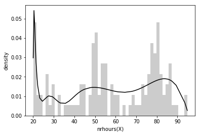
Figure 2: Failure of the binning method for nrhours

Q2: How does supervised discretisation compare to the unsupervised regime?

Generally speaking, all densities, including ones that are outside well-known families and are non-uniform (e.g., Figure 1a and Table2) were approximated satisfactorily by unsupervised methods. Approximations by supervised schemes, unsurprisingly, performed worse, in general, as the goal of the discretisation was not an optimal polynomial learner; e.g., the previously discussed figure 2. When limited to simpler distributions, such as Gaussians, however, the method performed on par or and, in some cases in the happiness dataset, even better than its unsupervised counterpart.

In the unsupervised regime, binning based on equal-frequency was often preferred to equal-width, see Table 1 which highlights the percentage of the equal frequency method being used for each dataset. Equal-Width binning, on the other hand, was selected when a small number of bins was able to model the density. This is natural as a small number of bins implies that the underlying distribution is not hard to approximate. If the distributions get more complicated, binning based on equal frequency can model the more complex relations better as it is not dependent on an attribute’s spread of values.

Q3: How does the piecewise polynomial approximation fare overall?

As can be surmised from the above discussions, the PP paradigm is a robust learning strategy for arbitrarily complex PDFs, provided the discretisation is satisfactory. (Both points are illustrated by Figure1a, and unsupervised schemes are a safe option to ensure satisfactory discretisation.)

Rule Learning

family(C)	prec	Neg	Pred	Rules
Sup: Auto	0.909	0.581	2.691	8
Sup: 5 Bins	1.0	0.741	2.871	6.6
Sup: 7 Bins	1.0	0.874	2.884	6.14
Unsup: best	0.966	0.598	3.179	10.6
Unsup: 5 bins	1.0	1.070	3.344	8.4
Unsup: 7 bins	1.0	1.562	3.617	6.429

Table 2: Rules learned for all interval instances of the family attribute. We compare our unsupervised framework against the extended supervised version. Auto denotes the automatic stopping criterion of the Distance discretisation. The table columns are: prec = Avg Rule precision over all bins, Neg = Avg number of negations in a rule body, Pred = Avg number of predicates in a rule body, Rules = Avg number of rules in one theory.

Q4: How compact are the learned rules?
We admit that compactness is not always a sign of interpretability, and, therefore, simply report on our empirical observations. As can be seen in Table 2, supervised discretisation yields more compact rules than the unsupervised regime: Given the same number of bins, the learned rules are overall shorter, contain fewer negations, and the programs are smaller, too.

A final observation worth reporting is with regards to data preprocessing. A large number of duplicate and missing values seem to lead to lengthy rules in the induced program. Interestingly, regardless of the regime (supervised vs unsupervised), the learned rules for the concerning attributes are almost syntactically identical for each bin size, in clear contrast to table 2. On the one hand, this calls for greater data preprocessing, which is not surprising. Conversely, perhaps the lack of compactness and the syntactic similarity across all regimes could be a diagnostic feature for data preprocessing, an investigation of which we leave for the future.

Example Programs

Here, we display some sample programs that were compiled after multiple runs of ProbFOIL with different attributes as targets. The polynomial weights have been omitted for readability. (See, for example, the PP density for $\tt int\_low$ from our prior discussions, and the multivariate case below.)

A sample program learned for the university data consists of rules such as:

intelligence1 :- intelligence(I),ininterval(I,51,60)intelligence2 :- intelligence(I),ininterval(I,60,72)nrhours2(C) :- nrhours(C,N),ininterval(N,35,50).satisfaction_mid(C) :- intelligence(I),ininterval(I,50,60),\+difficulty_hard(C).grade_high(C) :- difficulty_easy(C), \+intelligence2,\+nrhours2(C), \+intelligence1. A sample program learned for the happiness data consists of rules such as:

trust4(A) :- trust(A,I), ininterval(I,0.07857,  0.1044).happiness1(A) :- economy1(A), trust4(A).happiness1(A) :- freedom6(A), economy1(A).happiness6(A) :- health4(A), family2(A).happiness6(A) :- inregion_central_and_eastern_europe(A),trust4(A), health3(A).

Querying

Querying over such hybrid programs follows the syntax of the original ProbLog language. Given some evidence and a query, the success probability is calculated. Imagine, for example, that we want to determine the probability that the happiness of Slovakians is in happiness6. As Slovakia is an Eastern European country we add the evidence:

evidence(inregion_central_and_eastern_europe(slovakia)). To formulate the query, we ask:

query(happiness6(slovakia)). ProbLog then evaluates the query by combining the probability of happiness6 with the corresponding rules. The ininterval relation for each continuous relation (health4, family2, trust4, health3 and happiness6) calls an external function that calculates the integrated probability. Those probabilities are then returned to ProbLog where they are combined with the evidence and the rest of the program to generate the final probability, in this case, $0.143$.

As an illustration of multivariate continuous relations, we define a new predicate and add it to the program:

(4.44 -17.42*X + 19.66*X^2) * (-0.12+0.58*Y +0.52*Y^2)::social(X,Y)social1:-social(X,Y),ininterval(X,0.4,0.5),ininterval(Y,0.42,0.7).

We, furthermore add the new relation to the rules so that it is taken into account for our example query:

happiness6 :- health4, family2, social1.

The new program is evaluated and returns the revised probability 0.135.

Conclusions

To the best of our knowledge, this is the first attempt to articulate a compositional PLP framework for arbitrarily complex distributions from continuous data. It contributes an algorithmic framework that learns piecewise polynomial representations which are then related to obtain probabilistic logic programs, along with effective symbolic inference. In our view, it takes a step towards a difficult challenge, and the declarative/interpretability aspect of the paradigm will be attractive for reasoning and learning over continuous data.

References

- [Albarghouthi et al. 2017] Albarghouthi, A.; D’Antoni, L.; Drews, S.; and Nori, A. 2017. Quantifying program bias. arXiv preprint arXiv:1702.05437.
- [Baldoni et al. 2011] Baldoni, V.; Berline, N.; De Loera, J.; Köppe, M.; and Vergne, M. 2011. How to integrate a polynomial over a simplex. Mathematics of Computation 80(273):297–325.
- [Baldoni et al. 2014] Baldoni, V.; Berline, N.; De Loera, J. A.; Dutra, B.; Köppe, M.; Moreinis, S.; Pinto, G.; Vergne, M.; and Wu, J. 2014. A user’s guide for latte integrale v1. 7.1. Optimization 22:2.
- [Baral, Gelfond, and Rushton 2009] Baral, C.; Gelfond, M.; and Rushton, J. N. 2009. Probabilistic reasoning with answer sets. TPLP 9(1):57–144.
- [Belle, Passerini, and Van den Broeck 2015] Belle, V.; Passerini, A.; and Van den Broeck, G. 2015. Probabilistic inference in hybrid domains by weighted model integration. In Proceedings of 24th International Joint Conference on Artificial Intelligence (IJCAI), 2770–2776.
- [Bellodi and Riguzzi 2011] Bellodi, E., and Riguzzi, F. 2011. Learning the structure of probabilistic logic programs. In International Conference on Inductive Logic Programming, 61–75. Springer.
- [Cerquides and De Màntaras 1997] Cerquides, J., and De Màntaras, R. L. 1997. Proposal and empirical comparison of a parallelizable distance-based discretization method. In KDD, 139–142.
- [Chavira and Darwiche 2008] Chavira, M., and Darwiche, A. 2008. On probabilistic inference by weighted model counting. Artificial Intelligence 172(6-7):772–799.
- [Chen, Muggleton, and Santos 2008] Chen, J.; Muggleton, S.; and Santos, J. 2008. Learning probabilistic logic models from probabilistic examples. Machine learning 73(1):55–85.
- [Chistikov, Dimitrova, and Majumdar 2015] Chistikov, D.; Dimitrova, R.; and Majumdar, R. 2015. Approximate counting in smt and value estimation for probabilistic programs. In TACAS, volume 9035. ACTA INFORMATICA. 320–334.
- [De Raedt and Kimmig 2015] De Raedt, L., and Kimmig, A. 2015. Probabilistic (logic) programming concepts. Machine Learning 100(1):5–47.
- [De Raedt et al. 2015] De Raedt, L.; Dries, A.; Thon, I.; Van den Broeck, G.; and Verbeke, M. 2015. Inducing probabilistic relational rules from probabilistic examples. In Proceedings of 24th international joint conference on artificial intelligence (IJCAI), 1835–1842.
- [De Raedt, Kimmig, and Toivonen 2007] De Raedt, L.; Kimmig, A.; and Toivonen, H. 2007. Problog: A probabilistic prolog and its application in link discovery. In Proceedings of the 20th international joint conference on Artifical intelligence, 2468–2473.
- [Deville and Lau 1994] Deville, Y., and Lau, K.-K. 1994. Logic program synthesis. The Journal of Logic Programming 19:321–350.
- [Dheeru and Karra Taniskidou 2017] Dheeru, D., and Karra Taniskidou, E. 2017. UCI machine learning repository.
- [Dougherty et al. 1995] Dougherty, J.; Kohavi, R.; Sahami, M.; et al. 1995. Supervised and unsupervised discretization of continuous features. In Machine learning: proceedings of the twelfth international conference, volume 12, 194–202.
- [Džeroski, Cestnik, and Petrovski 1993] Džeroski, S.; Cestnik, B.; and Petrovski, I. 1993. Using the m-estimate in rule induction. Journal of computing and information technology 1(1):37–46.
- [Fierens et al. 2011] Fierens, D.; Van den Broeck, G.; Thon, I.; Gutmann, B.; and De Raedt, L. 2011. Inference in probabilistic logic programs using weighted CNF’s. In Proceedings of UAI, 211–220.
- [Garcia et al. 2013] Garcia, S.; Luengo, J.; Sáez, J. A.; Lopez, V.; and Herrera, F. 2013. A survey of discretization techniques: Taxonomy and empirical analysis in supervised learning. IEEE Transactions on Knowledge and Data Engineering 25(4):734–750.
- [Getoor et al. 2001] Getoor, L.; Friedman, N.; Koller, D.; and Pfeffer, A. 2001. Learning probabilistic relational models. In Relational data mining. Springer. 307–335.
- [Gulwani 2010] Gulwani, S. 2010. Dimensions in program synthesis. In Proceedings of the 12th international ACM SIGPLAN symposium on Principles and practice of declarative programming, 13–24. ACM.
- [Gutmann et al. 2011] Gutmann, B.; Thon, I.; Kimmig, A.; Bruynooghe, M.; and De Raedt, L. 2011. The magic of logical inference in probabilistic programming. TPLP 11:663–680.
- [Gutmann, Jaeger, and De Raedt 2010] Gutmann, B.; Jaeger, M.; and De Raedt, L. 2010. Extending problog with continuous distributions. In ILP, volume 6489, 76–91. Springer.
- [Gutmann, Thon, and De Raedt 2011] Gutmann, B.; Thon, I.; and De Raedt, L. 2011. Learning the parameters of probabilistic logic programs from interpretations. In ECML/PKDD (1), 581–596.
- [Heckerman, Geiger, and Chickering 1995] Heckerman, D.; Geiger, D.; and Chickering, D. 1995. Learning Bayesian networks: The combination of knowledge and statistical data. Machine Learning 20:197–243.
- [Kass and Wasserman 1995] Kass, R. E., and Wasserman, L. 1995. A reference bayesian test for nested hypotheses and its relationship to the schwarz criterion. Journal of the american statistical association 90(431):928–934.
- [Landwehr, Kersting, and De Raedt 2005] Landwehr, N.; Kersting, K.; and De Raedt, L. 2005. nfoil: integrating naïve bayes and foil. In Proceedings of the twentieth national conference on artificial intelligence (AAAI-05), 795–800.
- [Lauritzen and Jensen 2001] Lauritzen, S. L., and Jensen, F. 2001. Stable local computation with conditional gaussian distributions. Statistics and Computing 11(2):191–203.
- [López-Cruz, Bielza, and Larrañaga 2014] López-Cruz, P. L.; Bielza, C.; and Larrañaga, P. 2014. Learning mixtures of polynomials of multidimensional probability densities from data using b-spline interpolation. International Journal of Approximate Reasoning 55(4):989–1010.
- [Milch et al. 2005] Milch, B.; Marthi, B.; Russell, S. J.; Sontag, D.; Ong, D. L.; and Kolobov, A. 2005. BLOG: Probabilistic models with unknown objects. In Proc. IJCAI, 1352–1359.
- [Muggleton 1995] Muggleton, S. 1995. Inverse entailment and progol. New generation computing 13(3):245–286.
- [Murphy 1999] Murphy, K. P. 1999. A variational approximation for bayesian networks with discrete and continuous latent variables. In UAI, 457–466.
- [Murphy 2012] Murphy, K. 2012. Machine learning: a probabilistic perspective. The MIT Press.
- [Nitti et al. 2016] Nitti, D.; Ravkic, I.; Davis, J.; and De Raedt, L. 2016. Learning the structure of dynamic hybrid relational models. In 22nd European Conference on Artificial Intelligence (ECAI) 2016, volume 285, 1283–1290.
- [Quinlan 1990] Quinlan, J. R. 1990. Learning logical definitions from relations. Machine learning 5(3):239–266.
- [Raedt et al. 2016] Raedt, L. D.; Kersting, K.; Natarajan, S.; and Poole, D. 2016. Statistical relational artificial intelligence: Logic, probability, and computation. Synthesis Lectures on Artificial Intelligence and Machine Learning 10(2):1–189.
- [Raghavan, Mooney, and Ku 2012] Raghavan, S.; Mooney, R. J.; and Ku, H. 2012. Learning to read between the lines using bayesian logic programs. In Proceedings of the 50th Annual Meeting of the Association for Computational Linguistics: Long Papers-Volume 1, 349–358. Association for Computational Linguistics.
- [Ravkic, Ramon, and Davis 2015] Ravkic, I.; Ramon, J.; and Davis, J. 2015. Learning relational dependency networks in hybrid domains. Machine Learning 100(2-3):217–254.
- [Richardson and Domingos 2006] Richardson, M., and Domingos, P. 2006. Markov logic networks. Machine learning 62(1):107–136.
- [Sanner and Abbasnejad 2012] Sanner, S., and Abbasnejad, E. 2012. Symbolic variable elimination for discrete and continuous graphical models. In AAAI.
- [Schoenmackers et al. 2010] Schoenmackers, S.; Etzioni, O.; Weld, D. S.; and Davis, J. 2010. Learning first-order horn clauses from web text. In Proceedings of the 2010 Conference on Empirical Methods in Natural Language Processing, 1088–1098. Association for Computational Linguistics.
- [Shenoy and West 2011] Shenoy, P. P., and West, J. C. 2011. Inference in hybrid bayesian networks using mixtures of polynomials. International Journal of Approximate Reasoning 52(5):641–657.
- [Shenoy 2012] Shenoy, P. P. 2012. Two issues in using mixtures of polynomials for inference in hybrid bayesian networks. International Journal of Approximate Reasoning 53(5):847–866.
- [Speichert 2017] Speichert, S. 2017. Learning Hybrid Relational Rules with Piecewise Polynomial Weight Functions for Probabilistic Logic Programming. Master’s thesis, The University of Edinburgh, Scotland.
- [Zettlemoyer, Pasula, and Kaelbling 2005] Zettlemoyer, L. S.; Pasula, H.; and Kaelbling, L. P. 2005. Learning planning rules in noisy stochastic worlds. In AAAI, 911–918.