Incorporating a soft ordered phase into an amorphous configuration enhances its uniform plastic deformation under shear

Abstract

Amorphous materials of homogeneous structures usually suffer from nonuniform deformation under shear, which can develop into shear localization and eventually destructive shear band. One approach to tackle this issue is to introduce an inhomogeneous structure containing more than one phase, which can reduce the local nonuniform shear deformation and hinder its percolation throughout the system. Using thermostated molecular dynamics (MD) simulations, we compare the deformation behavior between a homogeneous amorphous mixture of bidisperse disc particles, interacting via an $n-6$ Lennard-Jones potential of tunable softness, with an inhomogeneous one containing an evenly-distributed ordered phase. We change the population ratio of large to small particles to create a homogeneous or an inhomogeneous mixture, where the softness of a chosen phase can be manually adjusted by specifying $n$ of the interparticle potential. Results of applying extensive quasistatic shear on the prepared mixtures reveal that the inhomogeneous amorphous mixture containing a soft ordered phase overall deforms more uniformly than the homogeneous one, which indicates that both the structure inhomogeneity and the inter-phase softness variance play important roles in enhancing the uniformity of the plastic deformation under shear.

I Introduction

Homogeneous amorphous materials such as bulk metallic glasses are known for exhibiting superior mechanical properties than their crystalline siblings. However, a significant disadvantage of amorphous materials is their low ductility, due to nonuniform shear deformation, which causes premature and unpredictable failure and greatly limits their industrial applications Ashby and Greer (2006); Hufnagel et al. (2016). Recently, introducing an ordered phase into an amorphous material to make the engineered structure inhomogeneous have been shown to improve their mechanical properties, for example, embedding an isolated and soft crystal phase containing dendrites in a bulk metallic glass matrix to enhance tensile ductility Hays et al. (2000); Szuecs et al. (2001); Hofmann et al. (2008a, b); Chen et al. (2012); Liu et al. (2012), and distributing polycrystalline metallic alloys within amorphous shells to raise mechanical strength and restrict shear localization Wu et al. (2017).

In this study, we propose a mesoscale model of mixing 2D bidisperse disc particles to study the shear deformation behavior of an amorphous configuration containing an ordered phase using molecular dynamics (MD) simulations. In our model of 2D amorphous materials, we prepare a homogeneous or an inhomogeneous amorphous/ordered configuration by mixing $50-50$ or $90-10$ small and large $12-6$ Lennard-Jones (LJ) disc particles, which allows the system to form an amorphous or a partially amorphous structure under thermal equilibrium Hamanaka and Onuki (2006, 2007). We set the interparticle interaction to be Lennard-Jones for the potential has long been used to study amorphous materials including metallic glasses Schun and Lund (2003); Ogata et al. (2006); Zhang et al. (2013). We then identify particles in the amorphous phase or the ordered phase based on the values of their disorder parameter. We alter the strength of a chosen phase by assigning the particles belonging to it proper interparticle softness, using an $n-6$ Lennard-Jones (LJ) potential Shi et al. (2011). We choose $n=8$ to make particles in the ordered phase softer than those in the amorphous phase. Finally, we apply quasistatic shear on the prepared configurations and calculate the uniformity of their deformation under extensive shear.

We investigated the difference in shear deformation between a homogeneous and an inhomogeneous configurations and demonstrate that an inhomogeneous configuration favors more uniform shear deformation due to the spatial and strength heterogenity between the two phases. Specifically, our model shows that introducing an ordered phase into an amorphous phase helps the inhomogeneous system deform more uniformly under shear than a homogeneous single-phased system when the applied shear strain is small. For large shear strain, the difference in softness between the two phases also plays an important role to further enhance the uniform plastic deformation. Our MD simulation results offer evidence supporting the improved ductility in mesoscale reported in experiments of amorphous materials Hays et al. (2000); Szuecs et al. (2001); Hofmann et al. (2008a, b); Chen et al. (2012); Liu et al. (2012); Wu et al. (2017).

Below we elaborate on the 2D model of amorphous materials and the MD simulation methods in section II, followed by quantitative results of comparing the deformation behavior of homogeneous and inhomogeneous configurations under quasistatic shear in section III. We conclude our study in section IV.

II Numerical simulation method

Our MD method includes two parts: 1) generating a homogeneous or inhomogeneous initial amorphous configuration and 2) applying quasistatic shear on it. To create an initial configuration, we first pick up an equilibrium configuration in a liquid state where particles interacting via the $12-6$ LJ potential and cool it down to a solid temperature. Here temperature is defined as the total kinetic energy divided by degrees of freedom of the system. Then we assign particles different softness according to their disorder parameter and prepare boundary particles. Finally, we relax the configuration sandwiched by the boundary particles at the same solid temperature. To test the deformation uniformity of the prepared initial configuration, we apply quasistatic shear by moving the boundary particles stepwise followed by thermostated relaxation and calculate the average deviation of uniform deformation of the sheared configuration. For each system setup, we use at least ten independent initial conditions to obtain the averaged results. The details are given below.

II.1 Preparation of an initial configuration

II.1.1 System geometry

Our system is a mixture of total $N=N_{s}+N_{l}$ circular particles interacting via the finite-range, pairwise-additive LJ potential. Specifically, it contains $N_{s}$ small particles of diameter $d_{s}$ and $N_{l}$ large particles of diameter $d_{l}$, with the diameter ratio $r=1.4$ to avoid artificial crystallization in 2D. We use $N=1000$ throughout this study. The masses of the small particles $m_{s}$ and the large particles $m_{l}$ are identical. The system occupies a square simulation box of size $L$ on the $xy$-plane, where $x$ is the horizontal axis and $y$ is the vertical one. For a given particle number $N$ and particle diameters $d_{s}$ and $d_{l}$, the box size is determined from the condition that the configuration has a fixed area packing fraction $\phi=0.793$ or soft-core packing fraction of LJ potential $\phi_{s}=1.0$. where $\phi$ and $\phi_{s}$ are defined as

$${\phi_{s}}={{\pi\left[{{N_{s}}{{\left({\frac{{{2^{1/6}}{d_{s}}}}{2}}\right)}^{2}}+{N_{l}}{{\left({\frac{{{2^{1/6}}{d_{l}}}}{2}}\right)}^{2}}}\right]}\mathord{\left/{\vphantom{{\pi\left[{{N_{s}}{{\left({\frac{{{2^{1/6}}{d_{s}}}}{2}}\right)}^{2}}+{N_{l}}{{\left({\frac{{{2^{1/6}}{d_{l}}}}{2}}\right)}^{2}}}\right]}{{L^{2}}}}}\right.\kern-1.2pt}{{L^{2}}}}={2^{1/3}}\phi.$$ (1)

The value ${2^{1/6}}{d_{s}}$ or ${2^{1/6}}{d_{l}}$ is where the $12-6$ LJ potential reaches its minimal, detailed below.

II.1.2 Interparticle Lennard-Jones potential

We choose the finite-range, pairwise additive LJ potential to build our amorphous model for it has been widely used to study amorphous systems Schun and Lund (2003); Ogata et al. (2006); Zhang et al. (2013). To create a softness difference between the amorphous and ordered phases in an inhomogeneous amorphous configuration, we choose a tunable $n-6$ LJ potential Shi et al. (2011)

$$V_{LJ}^{n-6}({r_{ij}})=\left[{4\epsilon\left({\lambda{{(\frac{{{d_{ij}}}}{{{r_{ij}}}})}^{n}}-\alpha{{(\frac{{{d_{ij}}}}{{{r_{ij}}}})}^{6}}}\right)-{c_{ij}}}\right]\Theta(\frac{{{r_{cut}}}}{{{r_{ij}}}}-1),$$ (2)

where $\epsilon$ is the characteristic energy scale, $\lambda=\frac{3}{2}[{{{2^{(n/6)}}}\mathord{\left/{\vphantom{{{2^{(n/6)}}}{(n-6}}}\right.\kern-1.2pt}{(n-6}})]$, $\alpha=n/[2(n-6)]$, $r_{ij}$ is the separation between particles $i$ and $j$, ${d_{ij}}=\frac{1}{2}({d_{i}}+{d_{j}})$ is their average diameter, ${c_{ij}}=4\epsilon[\lambda{({{{d_{ij}}}\mathord{\left/{\vphantom{{{d_{ij}}}{{r_{cut}}}}}\right.\kern-1.2pt}{{r_{cut}}}})^{n}}-\alpha{({{{d_{ij}}}\mathord{\left/{\vphantom{{{d_{ij}}}{{r_{cut}}}}}\right.\kern-1.2pt}{{r_{cut}}}})^{6}}]$ is a constant that guarantees $V_{LJ}^{n-6}({r_{ij}})\to 0$ as $r_{ij}\to{r_{cut}}$, and $\Theta(x)$ is the Heaviside step function. We use ${r_{cut}}=3.2{d_{s}}$, where $d_{s}$ is the diameter of small particles and $n=8$ for the soft $V_{LJ}^{8-6}$ LJ potential or $n=12$ for the well-known stiff $V_{LJ}^{12-6}$ LJ potential.

II.1.3 Tuning inhomogeneity and softness

The whole process of preparing a homogeneous or inhomogeneous initial configuration for our amorphous model can be summarized as follows. We (a) create a randomly packed initial configuration of circular particles without interparticle overlap; (b) equilibrate the system at a liquid temperature $T_{l}$ to relax it; (c) pick up a relaxed liquid configuration and equilibrate it again at a lower solid temperature $T_{s}$; (d) attach boundary particles to the relaxed solid configuration and reassign the interparticle interactions of all particles based on the value of their disorder parameters; (e) equilibrate the sandwiched solid configuration one last time at $T=T_{s}$.

The MD simulations in this study use the diameter $d_{s}$ and mass $m_{s}$ of the small particles and the interparticle potential amplitude $\epsilon$ as the reference length, mass, and energy scales. Mass $m_{l}$ of the large particles is the same as $m_{s}$. As a result, the unit of time $t$ is ${d_{s}}\sqrt{{m_{s}}/\epsilon}$. We control the temperature $T$ of this system using the Nóse-Hoover thermostat with a thermostat moment of inertia $Q$ Nóse (1983); Frenkel and Smit (2001). Here temperature $T$ is defined as the total kinetic energy $\sum\nolimits_{i=1}^{N}{{\raise 3.01385pt\hbox{${{m_{i}}v_{i}^{2}}$}\!\mathord{\left/{\vphantom{{{m_{i}}v_{i}^{2}}2}}\right.\kern-1.2pt}\!\lower 3.01385pt\hbox{$2$}}}$ divided by degrees of freedom of the system and measured in units of $\epsilon/k_{B}$, where $m_{i}$ and $v_{i}$ are the mass and velocity of particle $i$, and $k_{B}$ is the Boltzmann’s constant. Degrees of freedom of the system is $2N-2$ or $2N-1$ for periodic boundary conditions in both $x$ and $y$ directions or only in the $x$ direction. To closely compare our results with those in the literature Hamanaka and Onuki (2006, 2007); Hamanaka et al. (2008); Shiba and Onuki (2010), we set $T=T_{l}=2.0$ and $T=T_{s}=0.2$ to study the system in a liquid state or a solid state, respectively. The unit of $Q$ is $m_{s}d_{s}^{2}$. The Newtonian equations of motion of a $N$ particle system excluding boundary particles if any are integrated using the velocity Verlet algorithm Allen and Tildesley (1989).

We perform a thermostated relaxation of the system excluding boundary particles after generating a random non-overlapped initial configuration and whenever making changes in the simulation temperature, introducing boundary particles or reassigning properties of particles for the pairwise $n-6$ LJ interparticle interactions. The relaxation of a random initial configuration at $T=T_{l}$ also erases any beginning memory from the system. We terminate the relaxation process when the temperature fluctuation decays to within $\pm 5\%$ of the required temperature.

It is known that by mixing bidisperse 2D particles with the population ratio $c=N_{l}/N$ increasing from $0$ to $0.5$, we can create structure from a single-crystal, a partially-amorphous (polycrystal) structure to an amorphous structure Hamanaka and Onuki (2006, 2007). To create a inhomogeneous amorphous configuration containing an ordered phase, we choose a partially-amorphous structure using $c=0.1$ and $N=1000$.

After generating a random initial configuration (see the Appendix for the implementing details), we equilibrate it at $T=T_{l}$. We then bring the temperature down to $T_{s}$ within a time interval $\Delta t=10^{5}$ to equilibrium the system again with periodic boundary conditions in both $x$ and $y$ directions and $Q=40.0$. Using the relaxed configuration at $T=T_{s}$, we calculate the disorder parameter $D_{j}$ of particle $j$ defined as Halperin and Nelson (1978); Nelson (2002); Yamamoto and Onuki (1997, 1998); Hamanaka and Onuki (2006, 2007)

$${D_{j}}=2\sum\limits_{k=1}^{{N_{b}}}{[1-\cos 6({\beta_{j}}-{\beta_{k}})]},$$ (3)

where $\beta_{j}$ is a local crystalline angle introduced by ${e^{6i{\beta_{j}}}}={{\sum\nolimits_{k=1}^{{N_{b}}}{{e^{6i{\theta_{jk}}}}}}\mathord{\left/{\vphantom{{\sum\nolimits_{k=1}^{{N_{b}}}{{e^{6i{\theta_{jk}}}}}}{\left|{\sum\nolimits_{k=1}^{{N_{b}}}{{e^{6i{\theta_{jk}}}}}}\right|}}}\right.\kern-1.2pt}{\left|{\sum\nolimits_{k=1}^{{N_{b}}}{{e^{6i{\theta_{jk}}}}}}\right|}}$, $i$ is the imaginary unit $\sqrt{-1}$ and $\theta_{jk}$ is the angle between the separation vector ${{\mathord{\buildrel{\lower 3.0pt\hbox{$\scriptscriptstyle\rightharpoonup$}}\over{r}}}_{j}}-{{\mathord{\buildrel{\lower 3.0pt\hbox{$\scriptscriptstyle\rightharpoonup$}}\over{r}}}_{k}}$ of particle $j$ and its bonded neighboring particle $k$ and the horizontal $x$ axis. Particle $k$ is considered bonded to particle $j$ as long as $\left|{{{\mathord{\buildrel{\lower 3.0pt\hbox{$\scriptscriptstyle\rightharpoonup$}}\over{r}}}_{j}}-{{\mathord{\buildrel{\lower 3.0pt\hbox{$\scriptscriptstyle\rightharpoonup$}}\over{r}}}_{k}}}\right|\leq 1.5{d_{jk}}$ Hamanaka and Onuki (2007). The summation runs over all $N_{b}$ bonded neighboring particles $k$ of particle $j$. The value of $D_{j}$ is zero if particle $j$ and its bonded neighbors form an ordered perfect hexagonal structure and increases if the structure becomes more disordered.

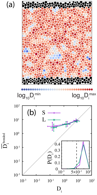
Figure 1: (color online) (a) A snapshot of an equilibrated configuration of $N=1000$ and $c=0.5$ at $T=T_{s}$. Particles are colored in shades from blue to red with increasing value of $log_{10}(D_{i})$. The color scale is divided evenly between the minimal and maximal disorder parameters, $log_{10}(D_{i}^{min})\approx-1.303$ and $log_{10}(D_{i}^{max})\approx 1.364$, in the system. Boundary particles are in black. (b) Averaged value of the disorder parameter of bonded neighbors of particle $i$ of disorder parameter value $D_{i}$. The inset shows the probability density distribution of $D_{i}$ with the same horizontal axis, and the total area below the two curves is one. The vertical dashed line shows a threshold $D_{t}=0.5$, separating ordered and disordered particles in this study. The data are obtained using ten relaxed configurations, where the results of small (S: purple) and large (L: green) particles are plotted separately.

Fig. 1(a) shows an equilibrated fully-amorphous configuration of $c=0.5$ at $T=T_{s}$, where particles are colored from blue to red with increasing $log_{10}(D_{i})$. Fig. 1(b) shows a weak positive correlation between $D_{i}$ of particle $i$ and the average $\bar{D}_{i}^{bonded}$ of the same quantity of its bonded neighbors, obtained by averaging ten relaxed initial conditions. We can see that particle $i$ can have ordered or disordered neighbors regardless of its $D_{i}$. The figure shows two curves of $\bar{D}_{i}^{bonded}$, for small or large particles, respectively. If we plot the probability density function $P(D_{i})$ of particle $i$ for small and large particles separately, as shown in the inset of Fig. 1(b), we can see quantitatively that almost all particles are very disordered with $D_{i}>0.5$, showing the configuration is indeed amorphous.

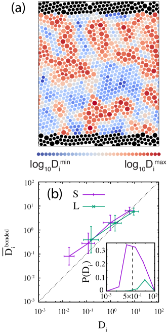
Figure 2: (color online) Same plots as in Fig. 1, except $c=0.10$. The color scale in (a) has a lower minimal and a similar maximal disorder parameters, $log_{10}(D_{i}^{min})\approx-2.012$ and $log_{10}(D_{i}^{max})\approx 1.411$, compared with those in Fig. 1(a).

Similarly, Fig. 2 shows an equilibrated partially-amorphous configuration of $c=0.1$ at $T=T_{s}$. We can observe in Fig. 2(a) that a majority of large particles are disordered and form the amorphous phase separating ordered islands made of small particles. The most ordered small particles form the cores of the ordered islands surrounded by less ordered particles. The degree of disorder of particles increases monotonically as a function of the distance measured from the ordered cores. Contrary to Fig. 1(b), Fig. 2(b) shows a strong positive correlation between $D_{i}$ of particle $i$ and its $\bar{D}_{i}^{bonded}$, also using ten relaxed initial conditions. We can clearly see that very ordered particles tend to have ordered neighbors, but highly disordered particles tend to have equally disordered neighbors, which gives the two curves positive slopes close to unity. Moreover, in the inset of Fig. 2(b), we can see quantitatively that almost all large particles are very disordered with $D_{i}>0.5$, while only about half small particles are in a similar disordered status.

The insets of Fig. 1 and Fig. 2 disclose the basic principle of how to build an homogeneous or inhomogeneous amorphous structure out of a mixture of small and large particles in this study: in a fully-amorphous configuration, all most all particles have their $D_{i}>D_{t}$, where $D_{t}=0.5$ is a threshold disorder value used in this study. On the other hand, in a partially-amorphous configuration, we can use $D_{i}<D_{t}$ to identify ordered particles, which form an ordered phase, and the rest particles form an amorphous phase. Of the ten initial configurations used in this study, the average number of ordered particles is $0.4406N$. The amorphous phases in homogeneous and inhomogeneous configurations are similar in terms of their disorder parameter distributions.

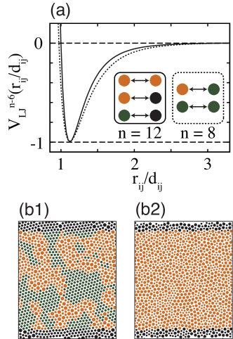
Figure 3: (color online) The $n-6$ LJ interparticle potential used in the 2D model of amorphous materials, shown in (a). The interaction between a soft ordered (green) particle and another soft ordered or stiff disordered (orange) particle is the soft $V_{LJ}^{8-6}$ LJ potential. The interaction between two stiff disordered particles or with a boundary particle (black) is the stiff $V_{LJ}^{12-6}$ LJ potential. Exemplary snapshots of an inhomogeneous and a homogeneous configurations are shown in (b1) and (b2), respectively.

For an inhomogeneous amorphous configuration, we assign the soft interparticle $V_{LJ}^{8-6}$ potential to the interaction between two ordered particles of ${D_{i}}\leq{D_{t}}$. We assign the same soft $V_{LJ}^{8-6}$ potential to the interaction between an ordered particle of ${D_{i}}\leq{D_{t}}$ and a disordered particle of ${D_{i}}>{D_{t}}$, happening at the interface between the ordered and amorphous phases. Moreover, the stiff interparticle $V_{LJ}^{12-6}$ potential governs the interaction between two disordered particles of ${D_{i}}>{D_{t}}$. Finally, the interaction between an ordered or disordered particle and a boundary particle is controlled by the same stiff $V_{LJ}^{12-6}$ potential. The boundary particles are image particles created using the periodic boundary condition in the vertical $y$ axis. We keep enough image particles so that the top and bottom boundaries have thickness equals $r_{cut}=3.2d_{s}$, and the total number of top or bottom boundary particles is about $3.2{d_{s}}\sqrt{N}$. Boundary particles are not thermostated, and we relax the prepared system sandwiched by boundary particles at $T=T_{s}$ again with periodic boundary condition in the horizontal $x$ direction and $Q=0.01$ before using it for the quasistatic shear tests. We observe only slight local position variation but no large-scale rearrangement of particles in the amorphous or ordered phase of the relaxed configuration. Two equilibrated snapshots of exemplary inhomogeneous and homogeneous amorphous configurations and the rules for interparticle interactions are shown in Fig. 3, where particles in soft-ordered and stiff-amorphous phases are colored in green and orange, respectively.

II.2 Quasistatic shear deformation

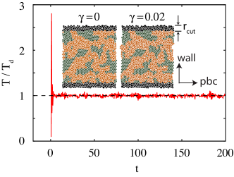
Figure 4: (color online) A sudden increase in temperature $T$ and its fluctuation, as a function of time $t$, corresponding to an increment of shear strain $\gamma$ of the system by $0.02$ in the quasistatic shear deformation. The quasistatic shear is done by evenly shifting the top and bottom boundary particles, within a thickness of $r_{cut}$, to the opposite directions, respectively. The perturbed temperature decays quickly to the desired value $T_{d}=T_{s}$ within the observation time interval.

We apply quasistatic shear strain on the prepared homogeneous and inhomogeneous amorphous configurations to test their plastic deformation behavior. To do this, at each step of the quasistatic shear, we shift the $x$ position of each top and bottom boundary particle by a small amount of $0.01L$ and $-0.01L$, respectively. The system heats up due to the perturbation from the moved boundary particles. Using a dimensionless MD time step $dt=0.001$ and the periodic boundary condition in the horizontal $x$ direction, we relax the system at temperature $T_{s}$ with the Nóse-Hoover thermostat of $Q=0.01$ integrated by the velocity Verlet algorithm until the standard deviation of temperature $T$, periodically calculated within a time interval of $2,500$ MD steps, decays to smaller than $0.03$, which corresponds to a temperature fluctuation within $\pm 5\%$ of the assigned temperature. Boundary particles are not thermostated and their positions stay fixed during the relaxation process. Fig. 4 demonstrates the decay of temperature fluctuation while applying this process on an exemplary inhomogeneous configuration. We repeat the two steps of shifting boundary particles and relaxation of the system at $T_{s}$ until a prescribed value of shear strain $\gamma$ is reached.

III Analysis of the uniformity of deformation under quasistatic shear

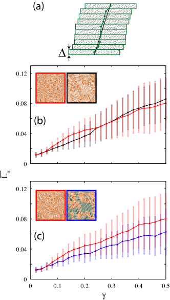
Figure 5: (color online) (a) The definition of the deviation of uniform deformation $L_{\sigma}$ which measures the difference between the averaged $x$ positions of $m=10$ sliced sections (connected green line), each with an identical thickness $\Delta$, of a given configuration and the $x$ positions of its calculated counterpart from the idealized uniformly-deformed profile (black line). (b) Averaged $L_{\sigma}$ of homogeneous configurations (red) and inhomogeneous configurations without softness inhomogeneity (black). In the inset, particles that are more ordered of an inhomogeneous configuration are semi-transparent. (c) Averaged $L_{\sigma}$ of the same homogeneous configurations (red) and the same inhomogeneous configurations except with softness inhomogeneity (blue). In the insets, the stiff and soft phases are colored in orange and green, respectively. For each case, the results are obtained using ten initial configurations.

As mentioned in the Introduction, we expect that an inhomogeneous amorphous configuration allows the system to shear more uniformly than a homogeneous one for the latter lack of the inhomogeneity of two phases with different softness to deter the emergence of shear localization. To measure the uniformity of shear deformation quantitatively, we calculate the deviation of uniform shear deformation $L_{\sigma}$ that measures how far a sheared configuration at a given strain $\gamma$ is away from its completely uniformly deformed counterpart, defined as

$${L_{\sigma}}(\gamma)=\sqrt{\frac{{\sum\nolimits_{i=1}^{m}{{{[{{\bar{x}}_{i}}(\gamma)\left|{{}_{y\in[{y_{i}}(\gamma)-{\Delta\mathord{\left/{\vphantom{\Delta 2}}\right.\kern-1.2pt}2},{y_{i}}(\gamma)+{\Delta\mathord{\left/{\vphantom{\Delta 2}}\right.\kern-1.2pt}2}]}}\right.-{x_{i}}(\gamma)]}^{2}}}}}{m}},$$ (4)

where $x_{i}$ and $y_{i}$ are calculated positions of the idealized uniform deformation profile, evenly divided into $m$ equal-sized stripes, $\Delta$ is the width of each stripe, and ${{{\bar{x}}_{i}}}$ is the averaged $x$ positions of particles whose $y$ positions located within ${y_{i}}-\frac{\Delta}{2}$ and ${y_{i}}+\frac{\Delta}{2}$ of stripe $i$. To make sure that the choice of $m$ has no influence on our conclusion, we have tried $m=5,10,20,30,40$ and $50$ and found that the values of $L_{\sigma}$ stay unchanged within negligible fluctuations. We therefore use $m=10$ throughout our analysis and ten trials with different initial conditions to calculate an averaged ${{\bar{L}}_{\sigma}}$ as a function of $\gamma$, as shown in Fig. 5(a).

Our amorphous model with tunable inhomogeneity allows us to compare the effects of introducing an inhomogeneous configuration and creating a softness difference between the two phases in the inhomogeneous configuration on the uniformity of shear deformation independently. We proceed with our investigation by two stages. First, to test the effect of introducing the inhomogeneous configuration, we compare the shear deformation behavior between an amorphous homogeneous configuration and a partially-amorphous inhomogeneous configuration, where the interparticle interactions are $V_{LJ}^{12-6}$ LJ potential in both cases. The results of the comparison is shown in Fig. 5(b). We can see clearly that introducing a configurational inhomogeneity effectively reduces nonuniform deformation when strain $\gamma$ is smaller than about $0.2$. When sheared further, the inhomogeneous configuration gradually loses to the homogeneous one.

Second, we incorporate the softness difference between the two phases of the inhomogeneous configuration, where now ordered particles interacting with another ordered or disordered particles via the soft $V_{LJ}^{8-6}$ LJ potential, and compare it with the homogeneous one as in the first stage. The results are shown in Fig. 5(c). Strikingly, the tuned inhomogeneous configuration deforms even more uniformly (smaller averaged $L_{\sigma}$) than the homogeneous one until the shear strain $\gamma$ reaches about $0.5$.

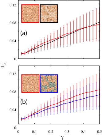
Figure 6: (color online) Averaged $L_{\sigma}$ as in Fig. 5 (b) and (c), except the results are obtained using fifty initial configurations for both cases.

Due to the large error bars in Fig. 5(b) and (c), we further verify the results using five times more initial configurations to verify the reliability of the observed trends. We confirm the trends stay the same and therefore saturate the data, as shown in Fig. 6.

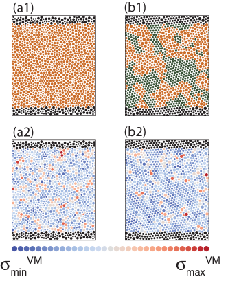
Figure 7: (color online) Snapshots of an equilibrated (a1) homogeneous and (b1) inhomogeneous configurations of $N=1000$ at $T=T_{s}$ and $\gamma=0.02$, colored by particle types (soft ordered: green; stiff disordered: orange) defined in the initial conditions. $c=0.1$ for the inhomogeneous configuration. Particles are colored in shades from blue to red with increasing value of the von Mises stress $\sigma^{VM}$ in (a2) and (b2) correspondingly. The color scale is relative to the minimal and maximal von Mises stresses $\sigma_{min}^{VM}$ and $\sigma_{max}^{VM}$ in each system.

To get a better insight into the deformation mechanism under shear of the homogeneous and inhomogeneous configurations, we calculate their per-particle von Mises stress, which is the deviatoric part of the stress tensor, defined as $\sigma_{i}^{VM}=\sqrt{{{(\sigma_{i}^{xx})}^{2}}+{{(\sigma_{i}^{yy})}^{2}}-\sigma_{i}^{xx}\sigma_{i}^{yy}+3{{(\sigma_{i}^{xy})}^{2}}}$ in 2D, where $\sigma_{i}^{ab}=-[m_{i}v_{i}^{a}v_{i}^{b}+\sum\nolimits_{j=1}^{{N_{p}}}{\frac{1}{2}r_{ij}^{a}f_{ij}^{b}}]$ for particle $i$ influenced by $N_{p}$ neighbors within ${r_{cut}}$ via the $n-6$ Lennard-Jones potential, $f_{ij}$ is the force acting on particle $i$ from its neighbor $j$, and $a,b\in[x,y]$ Thompson et al. (2009). The results are shown in Fig. 7. We observe that in a inhomogeneous configuration, particles subject to high $\sigma^{VM}$ shear stress mostly distribute within the amorphous phase, and the isolated soft-ordered phase disperses them so that they cannot coordinate to percolate through the whole system easily. Furthermore, we also calculate the local deviation from affine deformation, $D^{2}_{min}$, which identifies local irreversible particle shuffling in unit of $d_{s}^{2}$ Falk and Langer (1998). We show a comparison of $D^{2}_{min}$ between exemplary homogeneous and inhomogeneous configurations during the quasistatic shear strain interval $\gamma=[0.04,0.46]$ in Fig. 8. Both systems have similar probability density distribution $P(log_{10}(D_{min}^{2}))$ and a similar amount of particles are subject to irreversible shear deformations equal or greater than the same $max(D^{2}_{min})$ at $\gamma=0.46$. We can see clearly that particles with large $D^{2}_{min}$ concentrate on one side in the homogeneous system, responsible for the higher nonuniform deformation. On the other hand, similar particles are mostly distributed evenly within the amorphous phase, and the intermediate ordered phase hinders their percolation, which enhances the uniform deformation. Our calculations of $\sigma_{i}^{VM}$ and $D^{2}_{min}$ offer clear evidence that an inhomogeneous amorphous configuration can effectively deter nonuniform shear deformation than a homogeneous one.

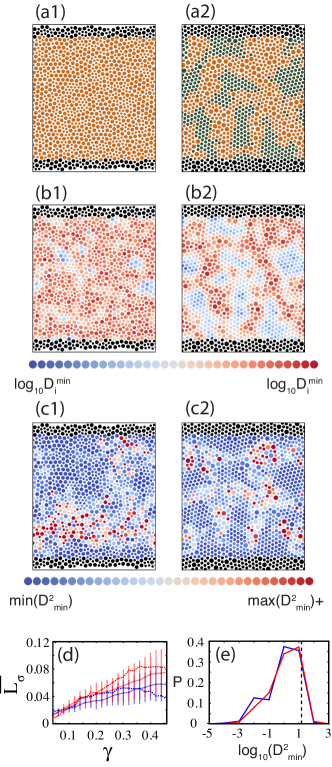
Figure 8: (color online) Snapshots of sheared homogeneous (a1) and inhomogeneous (a2) configurations at $\gamma=0.46$, colored by particle types (soft ordered: green; stiff disordered: orange). Particles of the homogeneous and inhomogeneous configurations are colored by the disorder parameter $D_{i}$ in (b1) with $log_{10}(D_{i}^{min})\approx-1.544$ and $log_{10}(D_{i}^{max})\approx 1.367$, and in (b2) with $log_{10}(D_{i}^{min})\approx-2.179$ and $log_{10}(D_{i}^{max})\approx 1.369$, respectively. (c1) and (c2) show particles colored by $D_{min}^{2}$ with a sampling radius of $1.49d_{s}$ and a reference configuration at $\gamma=0.04$ after eliminating homogeneous cell deformation. The color scale is evenly divided between $min(D_{min}^{2})=0$ and $max(D_{min}^{2})=15$, and particles having $D_{min}^{2}\geq max(D_{min}^{2})$ (homogeneous: $6.9\%$; inhomogeneous: $4.2\%$) are colored by the darkest red. ${{\bar{L}}_{\sigma}}$ of the homogeneous (dotted red) and inhomogeneous (dotted blue) configurations within $\gamma=[0.04,0.46]$ is shown in (d), having the averaged ${{\bar{L}}_{\sigma}}$ in Fig. 5(c) for reference. The corresponding probability density distribution $P(log_{10}(D_{min}^{2}))$, with $max(D_{min}^{2})$ indicated by the dashed line, is shown in (e).

IV Conclusions

In this study, we propose a 2D mixture of bidisperse particles to study the deformation behavior of homogeneous and inhomogeneous amorphous materials. A configuration modeling homogeneous amorphous materials is made of $50-50$ small and large particles. On the other hand, Our mesoscale model of inhomogeneous amorphous materials distributes large circular particles in a sea of small particles with a $1:9$ population ratio. In the inhomogeneous model, about half ($\approx 44\%$) small particles form an isolated and ordered phase. On the other hand, most large particles and the remaining half small particles together form an amorphous phase filling the space in between the ordered phase. To give the ordered or the amorphous phase proper mechanical softness as proposed in experiments on amorphous materials to improve their ductility, we introduce a tunable $n-6$ LJ potential. A particle in the soft-ordered phase interacts with another particle via the $8-6$ LJ potential. Two disordered particles interact with each other via the stiff $12-6$ LJ potential. We apply quasistatic shear on the homogeneous and inhomogeneous configurations by repeatedly moving the boundary particles with a stepwise shear strain of $0.02$, followed by thermostated relaxation.

Our simulation results show that when the applied shear strain $\gamma$ is small, the configurational inhomogeneity between the two phases in an inhomogeneous structure alone works well to improve uniform deformation. However, with increasing the shear deformation further, the difference in softness between the two phases plays an essential role to enhance the uniform shear behavior. In general, the inhomogeneous configurations deform more uniformly than the homogeneous ones. Our simplified model offers clear numerical evidence supporting the experimental results and could open a new quantitative approach to systematically improving the ductility of inhomogeneous amorphous materials including an ordered phase. For the future work, we will examine a hard ordered phase embedded in a soft disordered matrix and explore the optimal ordered/disordered area ratio that gives the best deformation uniformity, which will give a more complete picture of this study.

V Appendix: Generating a randomly packed configuration of particles

When conducting MD simulation in a liquid state, we start with an initial configuration at $\phi=0.793$ without overlap between particles. Practically, it is very difficult to generate such random initial configuration using a completely random process which places particles one by one. To avoid this issue, we first generate a mechanically stable (MS) packing of frictionless particles interacting via the finite-range pairwise-additive repulsive spring potential at area packing fraction $\phi=0.84$ ($\phi_{s}=1.06$), close to random-close packing density in 2D.

The MS packing of particles is generated using the procedure detailed in Gao et al. (2006). We start with a sparse initial configuration, and the procedure increases the sizes of the particles followed by energy minimization to remove overlap between particles. Periodic boundary conditions are implemented in both $x$ and $y$ directions. Occasionally, particles have to be shrunk if the energy minimization procedure fails to remove interparticle overlap. We repeat the two steps of particle size perturbation and energy minimization until all particles are force-balanced with their neighbors, and any attempt to increase particle size will result in an increase of the total energy of the system.

We then decrease $\phi$ from about $0.84$ ($\phi_{s}=1.06$) to $0.793$ ($\phi_{s}=1.0$) manually and run the thermostated MD simulation at $T=T_{l}$. Since the system is in a liquid state, it will soon forget it was from an MS state as long as it is fully relaxed.

VI acknowledgments

GJG acknowledges financial support from Shizuoka University startup funding. YJW acknowledges financial support from National Natural Science Foundation of China (NSFC No.11672299). We also thank Corey S. O’Hern for insightful comments.

References

- Ashby and Greer (2006) M. Ashby and A. Greer, Scripta Mater. 54, 321 (2006).
- Hufnagel et al. (2016) T. C. Hufnagel, C. A. Schuh, and M. L. Falk, Acta Mater. 109, 375 (2016).
- Hays et al. (2000) C. C. Hays, C. P. Kim, and W. L. Johnson, Phys. Rev. Lett. 84, 2901 (2000).
- Szuecs et al. (2001) F. Szuecs, C. P. Kim, and W. L. Johnson, Acta Mater. 49, 1507 (2001).
- Hofmann et al. (2008a) D. C. Hofmann, J.-Y. Suh, A. Wiest, G. Duan, M. Lind, M. D. Demetriou, and W. L. Johnson, Nature 451, 1085 (2008a).
- Hofmann et al. (2008b) D. C. Hofmann, J.-Y. Suh, A. Wiest, M. Lind, M. D. Demetriou, and W. L. Johnson, PNAS 105, 20136 (2008b).
- Chen et al. (2012) G. Chen, J. Cheng, and C. Liu, Intermetallics 28, 25 (2012).
- Liu et al. (2012) Z. Liu, R. Li, G. Liu, W. Su, H. Wang, Y. Li, M. Shi, X. Luo, G. Wu, and T. Zhang, Acta Mater. 60, 3128 (2012).
- Wu et al. (2017) G. Wu, K. Chan, L. Zhu, L. Sun, and J. Lu, Nature 545, 80 (2017).
- Hamanaka and Onuki (2006) T. Hamanaka and A. Onuki, Phys. Rev. E 74, 011506 (2006).
- Hamanaka and Onuki (2007) T. Hamanaka and A. Onuki, Phys. Rev. E 75, 041503 (2007).
- Schun and Lund (2003) C. A. Schun and A. C. Lund, Nat. Mater. 2, 449 (2003).
- Ogata et al. (2006) S. Ogata, F. Shimizu, J. Li, M. Wakeda, and Y. Shibutani, Intermetallics 14, 1033 (2006).
- Zhang et al. (2013) K. Zhang, M. Wang, S. Papanikolaou, Y. Liu, J. Schroers, M. D. Shattuck, and C. S. O’Hern, J. Chem. Phys. 139, 124503 (2013).
- Shi et al. (2011) Z. Shi, P. G. Debenedetti, F. H. Stillinger, and P. Ginart, J. Chem. Phys. 135, 084513 (2011).
- Nóse (1983) S. Nóse, Mol. Phys. 52, 255 (1983).
- Frenkel and Smit (2001) D. Frenkel and B. Smit, Understanding Molecular Simulation, 2nd ed. (Academic Press, Oxford, 2001).
- Hamanaka et al. (2008) T. Hamanaka, H. Shiba, and A. Onuki, Phys. Rev. E 77, 042501 (2008).
- Shiba and Onuki (2010) H. Shiba and A. Onuki, Phys. Rev. E 81, 051501 (2010).
- Allen and Tildesley (1989) M. P. Allen and D. J. Tildesley, Computer Simulation of Liquids, reprint edition ed. (Clarendon Press, Oxford, 1989).
- Halperin and Nelson (1978) B. I. Halperin and D. R. Nelson, Phys. Rev. Lett. 41, 121 (1978).
- Nelson (2002) D. R. Nelson, Defects and Geometry in Condensed Matter Physics, 1st ed. (Cambridge University Press, Cambridge, 2002).
- Yamamoto and Onuki (1997) R. Yamamoto and A. Onuki, J. Phys. Soc. Jpn. 66, 2545 (1997).
- Yamamoto and Onuki (1998) R. Yamamoto and A. Onuki, Phys. Rev. E 58, 3515 (1998).
- Thompson et al. (2009) A. P. Thompson, S. J. Plimpton, and W. Mattson, J. Chem. Phys. 131, 154107 (2009).
- Falk and Langer (1998) M. L. Falk and J. S. Langer, Phys. Rev. E 57, 7192 (1998).
- Gao et al. (2006) G. J. Gao, J. Bławzdziewicz, and C. S. O’Hern, Phys. Rev. E 74, 061304 (2006).