A minimal hyperbolic system for unstable shock waves

Abstract

We present a computational analysis of a 2$\times$2 hyperbolic system of balance laws whose solutions exhibit complex nonlinear behavior. Traveling-wave solutions of the system are shown to undergo a series of bifurcations as a parameter in the model is varied. Linear and nonlinear stability properties of the traveling waves are computed numerically using accurate shock-fitting methods. The model may be considered as a minimal hyperbolic system with chaotic solutions and can also serve as a stringent numerical test problem for systems of hyperbolic balance laws.

1 Introduction

We investigate a particular hyperbolic system of balance laws in one space dimension:

$$u_{t}+\left(f\left(u,\lambda\right)\right)_{x} = 0,$$ (1)

$$\lambda_{t} = \omega\left(u,\lambda\right),\quad t>0,x\in\mathbb{R},$$ (2)

where $u$ and $\lambda$ are the unknown functions, $f$ and $\omega$ are given flux and rate function, respectively, and subscripts $t$ and $x$ denote partial derivatives in time and space, respectively. We demonstrate numerically that the system possesses nontrivial dynamical properties. In particular, we show that its traveling-wave solutions can become unstable as a system parameter is varied, and that the instability manifests itself as an Andronov–Hopf bifurcation leading to a limit-cycle attractor. Further increase of the parameter results in a cascade of period-doubling bifurcations and the onset of apparently chaotic dynamics.

Much analysis of systems of the type (1-2) is due to Fickett [13, 14, 16, 15], who was the first to introduce it as an analog (or a toy model) of the reactive Euler equations of gas dynamics with the purpose of modeling the dynamics of detonations. A similar model which also included diffusive effects was proposed independently by Majda [32]. The Majda model has received much attention in the mathematics literature [49, 31, 21, 22, 30] as a prototype to study existence and stability of traveling waves. It must be pointed out that in the analyses of the Majda model only stable traveling waves have been found so far, to the best of our knowledge. In contrast, the model studied in the present work predicts instabilities, as pointed out originally in [11].

The Fickett model [13] has subsequently motivated various extensions and modifications [34, 43, 25, 10, 12, 9]. The principal aim of all of these works is to identify a minimal model that is capable of reproducing the rich set of dynamical properties of the full system of the reactive Euler equations. It is hoped that doing so might help in revealing the key mechanisms of the observed complex dynamics of the full system. As the recent publications mentioned above have demonstrated, the Fickett model indeed successfully reproduces most of the features of the full system. These results have also motivated the development of an asymptotic theory of gaseous detonations in [11] in which a reduced model is derived that is found to be very similar to the Fickett ad hoc model (1-2), however with a difference in the second equation – instead of $\lambda_{t}$, the asymptotic model has $\lambda_{x}$ (see also the earlier related work [36, 37, 6]). It was stated in [11] that in either case, the system possesses instabilities as long as the rate function $\omega$ is chosen that has the right properties. Further analysis of the system with $\lambda_{t}$ was not pursued by the authors of [11]. Here, we carry out a complete numerical investigation of such a system using the particular rate function $\omega$ from the asymptotic model of [11] as an example.

We also propose that (1-2) can serve as a numerical benchmark problem for systems of hyperbolic balance laws. Despite its simplicity, the system exhibits rather complex and sensitive dynamics of solutions. As such, it can be used as a stringent test problem for numerical algorithms that are to accurately reproduce stability properties in problems with complex dynamical features. As examples of such problems we mention detonations, shallow water flows over topographies, shock waves in the presence of body forces (e.g., gravitational or electromagnetic fields). A good numerical method must correctly reproduce neutral stability boundaries and development of instability as the boundary is crossed. For such problems, our model and the results reported here can be used as a relatively simple benchmark case.

The remainder of the paper is structured as follows. The model system and its main mathematical properties are introduced in Section 2. The traveling-wave solutions of the model are found in Section 3. The numerical algorithms used to calculate both linear and nonlinear dynamics of the system require the so-called shock-evolution equation, which is derived in Section 4. The linear stability of traveling waves and nonlinear dynamics are presented in Sections 5 and 6, respectively, while code verification results are given in Section 7. Conclusions are presented in Section 8.

2 The model system

In the original paper [13], Fickett proposed a simple ad hoc system of hyperbolic equations to qualitatively model the dynamics of detonation waves. To remind the reader, a detonation is a self-sustained shock wave propagating in a reactive medium such that the shock compression and heating triggers exothermic chemical reactions, and the thermal energy released in these reactions serves to support the motion of the shock [17]. Usually, detonations are modeled by the reactive Euler equations of gas dynamics which consist of conservation laws of mass, momentum and energy, and at least one equation that describes chemical heat release. Thus, in one spatial dimension, this is a hyperbolic system of at least four quasilinear equations. Analysis of detonations by means of the reactive Euler equations has received much attention and continues actively at present. See, for example, recent reviews [1, 2, 42, 7, 49, 5]. One of the key properties of gaseous detonations is their manifestly time-dependent and spatially complex dynamics. Thus arises the problem of understanding the physical mechanisms of such behavior and of the mathematical properties of the governing equations that are responsible for the observed complex dynamics.

Fickett’s model system can be written as follows:

$$u_{t}+\frac{1}{2}\left(u^{2}+q\lambda\right)_{x} =0,$$ (3)

$$\lambda_{t} =\omega\left(u,\lambda\right).$$ (4)

Here, the first equation is to play the role of the combined momentum–energy equation while the second is the rate equation for the chemical energy release, $q$ is the heat release parameter. The first equation of the model is a conservation law with a flux function $f\left(u,\lambda\right)$ in which the second variable $\lambda$ satisfies the ordinary differential equation (ODE) (4). The variable $\lambda$ measures the reaction progress, varying from $\lambda=0$ in the unburnt (ambient) state ahead of the shock to $\lambda=1$ in the burnt state far downstream of the shock.

We assume that the shock moves from left to right in the positive $x$ direction. Thus, if $x=x_{\mathrm{s}}\left(t\right)$ denotes the shock position at time $t$, the upstream unburnt state is at $x>x_{\mathrm{s}}\left(t\right)$, the reaction zone is at $x<x_{\mathrm{s}}\left(t\right)$, and the burnt state is reached asymptotically at $x\to-\infty$.

We choose the reaction rate following [11] as

$$\omega(u,\lambda)=\begin{cases}k(1-\lambda)\exp\left(\theta\left(\sqrt{q}u+q\lambda\right)\right),&x<x_{\mathrm{s}}\left(t\right),\\ 0,&x>x_{\mathrm{s}}\left(t\right),\end{cases}$$ (5)

where $k$ is the rate constant, $\theta$ is the activation energy, and $q$ is the same heat release parameter as in (3). This form of the rate function was derived from the reactive Euler equations in a particular asymptotic limit of weakly nonlinear waves in [11]. It must be emphasized however that our use of the function is outside the asymptotic theory and must be considered only as a particular case of Fickett’s analog system.

In vector form, system (3–4) can be written as

$$\bm{z}_{t}+\left(\bm{f}\left(\bm{z}\right)\right)_{x}=\bm{s}\left(\bm{z}\right),$$ (6)

where

$$\bm{z}=\left[\begin{array}[]{l}u\\ \lambda\end{array}\right],\quad\bm{f}=\left[\begin{array}[]{l}\frac{1}{2}u^{2}+\sigma\lambda\\ 0\end{array}\right],\quad\bm{s}=\left[\begin{array}[]{l}0\\ \omega\end{array}\right],$$

and $\sigma=q/2$ will also be used along with $q$. The Jacobian of $\bm{f}$,

$$\mathbf{A}=\left[\begin{array}[]{ll}u&\sigma\\ 0&0\end{array}\right],$$ (7)

has eigenvalues $\mu_{1}=u$ and $\mu_{2}=0$ with corresponding right eigenvectors $\bm{r}_{1}=[1,0]^{\mathrm{T}}$ and $\bm{r}_{2}=[1,-u/\sigma]^{\mathrm{T}}$. Clearly, the second characteristic field is linearly degenerate while the first is genuinely nonlinear as $\nabla\mu_{1}\cdot\bm{r}_{1}=1\neq 0$.

In nonconservative form, the system (3–4) becomes

$$u_{t}+uu_{x}+\sigma\lambda_{x} =0,$$ (8)

$$\lambda_{t} =\omega,$$ (9)

from which the characteristic form of the system readily follows by adding (9) multiplied by $\sigma$ to (8) multiplied by $u$ ((9) is already in the characteristic form):

$$\dot{p} =\sigma\omega \quad\text{on }\dot{x} =u,$$ (10)

$$\dot{\lambda} =\omega \quad\text{on }\dot{x} =0,$$ (11)

where $p=u^{2}/2+\sigma\lambda$, and the dots are used here and from now on to denote total time derivatives, e. g., $\dot{p}=dp/dt$.

For the numerical solution of (3–4), it is advantageous to move to a reference frame attached to the lead shock by using new coordinates $\xi=x-x_{\mathrm{s}}\left(t\right)$ and $\tau=t$. In this new reference frame, the shock is always at the same position, $\xi=0$, which serves as the right-end boundary of the reaction zone. Because no finite-differencing is made across the shock, the usual numerical shock smearing is removed in this formulation, which is its key advantage. Reusing the notation $x$ and $t$ in place of $\xi$ and $\tau$ and denoting the shock velocity as $D=\dot{x}_{\mathrm{s}}$, the governing equations in the shock-attached frame become:

$$u_{t}+\frac{1}{2}\left(\left(u-2D\right)u+q\lambda\right)_{x} =0,$$ (12)

$$\lambda_{t}-D\lambda_{x} =\omega.$$ (13)

Equations (12–13) must be supplemented with the Rankine–Hugoniot conditions for $u$ and $\lambda$ at the shock (see e.g., [28]). We denote the state variables right ahead of the shock (at position $x_{\mathrm{s}}^{+}$) by subscript “a” (for “ambient”), and the state variables right behind the shock (at position $x_{\mathrm{s}}^{-}$) by subscript “s” (for “shock”). We also assume for simplicity that the ambient (upstream) conditions ahead of the shock are $u_{\mathrm{a}}=0$ and $\lambda_{\mathrm{a}}=0$. The Rankine–Hugoniot condition for $\lambda$ is $\left[\lambda\right]=0$, where brackets denote the jump across the shock ($\left[z\right]=z^{+}-z^{-}$), because no reaction is assumed to take place inside the shock. As a result, we obtain

$$\lambda_{\mathrm{s}}=0.$$ (14)

The jump in $u$ in (12) satisfies

$$\left[\left(u-2D\right)u\right]+q\left[\lambda\right]=0,$$ (15)

which yields

$$u_{\mathrm{s}}=2D.$$ (16)

3 The traveling shock-wave solution

Next, we calculate the traveling-wave solutions of (12–13) (called ZND solutions after Zel’dovich [48], von Neumann [47], Döring [8]). Substituting $u=\bar{u}\left(x-\bar{D}t\right)$, $\lambda=\bar{\lambda}\left(x-\bar{D}t\right)$ into the system, with overbar denoting the steady state and $\bar{D}=\text{const}$, we obtain

$$\frac{d}{dx}\left(\frac{\bar{u}^{2}}{2}-\bar{D}\bar{u}+\frac{q}{2}\bar{\lambda}\right) =0,$$ (17)

$$\frac{d\bar{\lambda}}{dx} =-\frac{\bar{\omega}}{\bar{D}}.$$ (18)

From (17), we find the algebraic relation

$$\bar{u}^{2}-2\bar{D}\bar{u}+q\bar{\lambda}=\text{const}=\bar{u}_{\mathrm{s}}^{2}-2\bar{D}\bar{u}_{\mathrm{s}}+q\bar{\lambda}_{\mathrm{s}}=0\quad\text{(with }\bar{u}_{\mathrm{s}}=2\bar{D}\text{)}.$$

The root of this equation satisfying condition (16) is

$$\bar{u}=\bar{D}+\sqrt{\bar{D}^{2}-q\bar{\lambda}}.$$ (19)

Then, the spatial structure of the traveling-wave solution is found by substituting (19) into (18) and integrating the resultant ODE

$$\frac{d\bar{\lambda}}{dx}=-\frac{\bar{\omega}\left(\bar{u}\left(\bar{\lambda}\right),\bar{\lambda}\right)}{\bar{D}},$$ (20)

from $x=0$ to $x<0$ using $\bar{\lambda}\left(0\right)=0$.

Importantly, so far $\bar{D}$ remains unknown. As in the classical detonation theory [17], the steady detonation velocity is found using a special condition at a sonic point, where the flow speed relative to the shock becomes equal to the local sound speed. Equivalently, this sonic condition follows from the requirement that the solution remains regular everywhere in the post-shock region. For our particular case, this means that $\bar{u}\left(x\right)$ must remain sufficiently smooth everywhere at $x<0$. From (19) and (20), we find that

$$\frac{d\bar{u}}{dx} =\frac{1}{2}\frac{-q}{\sqrt{\bar{D}^{2}-q\bar{\lambda}}}\frac{d\bar{\lambda}}{dx}=\frac{1}{2}\frac{q\bar{\omega}}{\bar{D}\sqrt{\bar{D}^{2}-q\bar{\lambda}}}.$$ (21)

Therefore, this derivative can blow up if $\bar{D}^{2}-q\bar{\lambda}=0$ at any point where $\bar{\omega}\neq 0$. With our choice of the reaction rate, $\bar{\omega}$ vanishes only at $\bar{\lambda}=1$. Hence, to avoid any singularity in $\bar{u}$, we require that $\bar{D}^{2}-q\bar{\lambda}=0$ whenever $\bar{\lambda}=1$. This condition yields a unique value for the traveling-wave speed (called the Chapman–Jouguet, or CJ speed in detonation theory [17]),

$$\bar{D}=\sqrt{q}.$$ (22)

The pre-exponential factor, $k$, in (5) is a property of chemical reactions, related to the frequency of molecular collisions. It is customary in detonation theory to eliminate this parameter by rescaling the spatial coordinate such that a characteristic length scale is the so-called half-reaction length of the steady reaction zone, that is, the distance between the shock and the point where half of the chemical energy is released, i. e., $\bar{\lambda}=1/2$. Then, we find from (20) that with

$$k=\int_{0}^{1/2}\frac{\bar{D}}{\left(1-\bar{\lambda}\right)\exp\left(\theta\left(\sqrt{q}\bar{u}+q\bar{\lambda}\right)\right)}\,d\bar{\lambda},$$ (23)

$x=-1$ where $\bar{\lambda}=1/2.$

Figure 1 shows computed spatial profiles of $\bar{u}$ and $\bar{\lambda}$ at $q=4$ and varying activation energy $\theta\in\left\{0.5,1,2,5\right\}$. The plot demonstrates that as the value of the activation energy increases, the profile of $\bar{\lambda}$ develops a steeper slope near $x=-1$, implying an increased stiffness of the problem at large $\theta$.

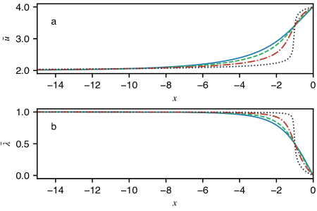
Figure 1: ZND profiles for $q=4$: a) velocity $\bar{u}$, b) reaction progress variable $\bar{\lambda}$, as $\theta$ is varied: $\theta=0.5$ (solid line), $\theta=1$ (dashed line), $\theta=2$ (dashed-dotted line), $\theta=5$ (dotted line). With increase of $\theta$ ZND profiles become steeper and approach “square-wave” structure, in which reaction effectively occurs in a narrow region near the lead shock at $x=0$.

4 Shock-evolution equation

The detonation speed, $D$, which is generally unknown for time-dependent solutions, appears explicitly in (12-13) in the shock-attached frame. Therefore, a method is needed to compute $D$ when solving the system numerically. As in the related previous work [20, 26, 44], in this subsection, we derive a shock-evolution equation (also called the “shock-change equation” [4, 15]) that is used subsequently to determine $D$ as part of the numerical algorithms that follow.

The evolution equation is derived by computing the rate of change of $u$ on the shock path by two different means. On the one hand, using the laboratory-frame equations (3-4), we find that

$$\dot{u}|_{\mathrm{s}}=\left(u_{t}+Du_{x}\right)|_{\mathrm{s}},$$ (24)

and eliminating $u_{t}$ from here using (3), it follows that

$$\dot{u}|_{\mathrm{s}}=\left((D-u)u_{x}-\sigma\lambda_{x}\right)|_{\mathrm{s}}.$$ (25)

On the other hand, $\dot{u}|_{\mathrm{s}}=du_{\mathrm{s}}/dt=2\dot{D}$ by the Rankine–Hugoniot condition (16), and therefore we find that the shock acceleration is given by

$$\dot{D}=\frac{1}{2}\left.\left((D-u)u_{x}+\frac{\sigma}{D}\omega\right)\right|_{\mathrm{s}}.$$ (26)

Here, we used the fact that no chemical reaction occurs in the shock, i.e., $\lambda_{\mathrm{s}}=0$ at all times, and therefore $0=\dot{\lambda}|_{\mathrm{s}}=\left(\lambda_{t}+D\lambda_{x}\right)|_{\mathrm{s}}=\left(\omega+D\lambda_{x}\right)|_{\mathrm{s}}$, and hence

$$\lambda_{x}|_{\mathrm{s}}=-\omega_{\mathrm{s}}/D.$$ (27)

Using (26), the detonation velocity, $D\left(t\right)$, can be evolved in time provided the right-hand side quantities are known. Among these quantities, all are known exactly in terms of $D$ through the Rankine–Hugoniot conditions, with the exception of $u_{x}|_{\mathrm{s}}$. The latter is approximated using one-sided finite differences for solutions with smooth profiles of $u$ near the shock. When the solution loses smoothness due to secondary shocks that can arise behind the lead shock and can catch up with it, $u_{x}|_{\mathrm{s}}$ blows up and hence (26) cannot be applied. The detonation velocity should be computed differently in that case, which we explain in Subsection 6.3.

5 Linear stability analysis

The first step in analyzing the dynamics of traveling-wave solutions of (12-13) is to understand their linear stability. In this section, we investigate the linear stability properties of the model employing the algorithm developed in [24] as well as the traditional method of normal modes. The neutral stability boundary in the plane of parameters $q$ and $\theta$ is determined. Note that $q$ and $\theta$ are the only free parameters of the problem and therefore the neutral boundary provides a complete stability diagram.

5.1 Algorithm for linear stability computations

Let $\bm{z}=\left(u,\lambda\right)^{\mathrm{T}}$ denote the vector of state variables. Then, expanding $\bm{z}$ and $D$ about their steady-state values, $\bm{z}=\bar{\bm{z}}(x)+\bm{z}^{\prime}(x,t)$, $D=\bar{D}+\psi^{\prime}(t)$, with primes denoting small perturbations, we arrive at the linearized equations

$$\bm{z}^{\prime}_{t}=-\bm{A}(\bar{\bm{z}})\bm{z}^{\prime}_{x}-\bm{B}(\bar{\bm{z}})\bm{z}^{\prime}+\frac{d\bar{\bm{z}}}{dx}\psi^{\prime},$$ (28)

where

$$\bm{A}=\begin{bmatrix}\bar{u}-\bar{D}&\sigma\\ 0&-\bar{D}\end{bmatrix},\quad\bm{B}=\begin{bmatrix}\frac{d\bar{u}}{dx}&0\\ -\bar{\omega}_{u}&-\bar{\omega}_{\lambda}\end{bmatrix},$$

in which the steady quantities are known with the partial derivatives of $\bar{\omega}$ being $\bar{\omega}_{u}=\theta\sqrt{q}\bar{\omega}$, $\bar{\omega}_{\lambda}=k\exp\left(\theta\left(\sqrt{q}\bar{u}+q\bar{\lambda}\right)\right)\,\left(\theta q(1-\bar{\lambda})-1\right)$, and the perturbations $u^{\prime}$, $\lambda^{\prime}$, and $\psi^{\prime}$ are to be found.

Linearization of the Rankine–Hugoniot conditions (14–16) gives

$$\lambda^{\prime}_{\mathrm{s}}=0,\quad u^{\prime}_{\mathrm{s}}=2\psi^{\prime},$$ (29)

and linearization of the shock-evolution equation (26) gives

$$\frac{d\psi^{\prime}}{dt}=\frac{1}{2}\left[\frac{qk\exp(2\theta\sqrt{q}\bar{D})(\theta\sqrt{q}\bar{D}-1)}{\bar{D}^{2}}\psi^{\prime}-\bar{D}u^{\prime}_{x}|_{\mathrm{s}}\right].$$ (30)

As mentioned earlier, the shock-evolution equation contains the unknown perturbation gradient, $u^{\prime}_{x}|_{\mathrm{s}}$, which must be approximated numerically using the known values of $u^{\prime}$ near the shock.

We now explain the algorithm that is used to integrate the linearized system [24]. Computations start with the evaluation of the following parameters: the value of self-sustained detonation velocity, $\bar{D}$, value of the pre-exponential factor, $k$, and the numerical reaction-zone length, $\mathcal{L}$, which is found by integrating (20) up to $\bar{\lambda}=\bar{\lambda}^{*}$:

$$\mathcal{L}\left(\bar{\lambda}^{*}\right)=\lceil I\rceil\text{ with }I=\int_{0}^{\bar{\lambda}^{*}}\frac{\bar{D}}{\bar{\omega}\left(\bar{u},\bar{\lambda}\right)}\,d\bar{\lambda},$$ (31)

where $\lceil\cdot\rceil$ is the ceiling function, $\bar{u}=\bar{u}\left(\bar{\lambda}\right)$ and $\bar{\omega}\left(\bar{u},\bar{\lambda}\right)$ are given by (19) and (5), and $\bar{\lambda}^{*}=1-\tau_{\lambda}$ with $\tau_{\lambda}$ being a prescribed tolerance measuring the deviation of $\bar{\lambda}^{*}$ from the chemical-equilibrium value $\bar{\lambda}=1$ to avoid the divergence of $I$ (to remind, $\bar{\omega}\sim 1-\bar{\lambda}$, which leads to a logarithmic divergence of the integral as $\bar{\lambda}^{*}\to 1$). For the following computations, we use $\tau_{\lambda}=10^{-6}$.

The computational domain is partitioned using a uniform grid of size $N$ with the grid size $\Delta x=1/N_{1/2}$, where $N_{1/2}$ is the resolution per half-reaction zone (recall that by (23), the half-reaction zone is unity), such that $N=N_{1/2}\mathcal{L}$. Figure 2a shows the schematics of the computational domain and the grid organization for the linear solver while Figure 2b shows the grid for the nonlinear solver, which is described in Subsection 6.1.

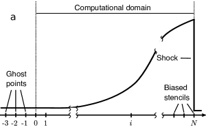
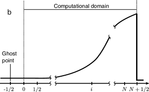
Figure 2: The sketches of the numerical grids for: a) linear solver; b) nonlinear solver (see Section 6). The sketched profile is $u$ as in a traveling-wave solution.

Once the grid partitioning is completed, the steady-state solution profiles are found by solving an initial-value problem for the ODE (20) with initial conditions at the shock given by the Rankine–Hugoniot conditions. We use the VODE solver [3] from scipy.integrate package [23] with a BDF (backward differencing formula) method of fifth order and relative and absolute tolerances set to $10^{-15}$. After the integration, all other steady-state quantities ($\bar{u}$, $\bar{\omega}$, $\bar{\omega}_{u}$, $\bar{\omega}_{\lambda}$, $d\bar{u}/dx$, and $d\bar{\lambda}/dx$) are computed.

Then, the linearized system is integrated by the method of lines:

$$\frac{d\bm{z}^{\prime}}{dt} =\widehat{\bm{L}}(\bar{\bm{z}},\bm{z}^{\prime}),\quad\text{for }i=0,\quad N-1,$$ (32)

$$\frac{d\psi^{\prime}}{dt} =\widehat{s}\left(\bar{\bm{z}},\bm{z}^{\prime}\right),$$ (33)

where $\widehat{\bm{L}}(\bar{\bm{z}},\bm{z}^{\prime})$ and $\widehat{s}(\bar{\bm{z}},\bm{z}^{\prime})$ are the finite-difference analogs of the right-hand sides of (28) and (30) in which spatial derivatives $\bm{z}^{\prime}_{x}$ are approximated using finite-difference formulas given next.

At points $i=0,\dots,N-3$, we compute left- and right-biased approximations of $\bm{z}^{\prime}_{x}$ using the fifth-order upwind method:

$$\left.\bm{z}_{x}^{\prime-}\right|_{x=x_{i}} =\frac{-2\bm{z}^{\prime}_{i-3}+15\bm{z}^{\prime}_{i-2}-60\bm{z}^{\prime}_{i-1}+20\bm{z}^{\prime}_{i}+30\bm{z}^{\prime}_{i+1}-3\bm{z}^{\prime}_{i+2}}{60\Delta x}+\mathcal{O}\left(\Delta x^{5}\right),$$ (34)

$$\left.\bm{z}_{x}^{\prime+}\right|_{x=x_{i}} =\frac{3\bm{z}^{\prime}_{i-2}-30\bm{z}^{\prime}_{i-1}-20\bm{z}^{\prime}_{i}+60\bm{z}^{\prime}_{i+1}-15\bm{z}^{\prime}_{i+2}+2\bm{z}^{\prime}_{i+3}}{60\Delta x}+\mathcal{O}\left(\Delta x^{5}\right),$$ (35)

To avoid the approximation of the spatial derivatives across the shock, at points $i=\{N-2,N-1,N\}$ we use biased stencils for finite-difference approximations [20]:

$$\left.\bm{z}^{\prime}_{x}\right|_{x=x_{N-2}}=\frac{-2\bm{z}^{\prime}_{N-5}+15\bm{z}^{\prime}_{N-4}-60\bm{z}^{\prime}_{N-3}+20\bm{z}^{\prime}_{N-2}+30\bm{z}^{\prime}_{N-1}-3\bm{z}^{\prime}_{N}}{60\Delta x}+\mathcal{O}\left(\Delta x^{5}\right),$$ (36)

$$\bm{z}^{\prime}_{x}|_{x=x_{N-1}}=\frac{-\bm{z}^{\prime}_{N-4}+6\bm{z}^{\prime}_{N-3}-18\bm{z}^{\prime}_{N-2}+10\bm{z}^{\prime}_{N-1}+3\bm{z}^{\prime}_{N}}{12\Delta x}+\mathcal{O}\left(\Delta x^{4}\right),$$ (37)

$$u^{\prime}_{x}|_{N}=\frac{-12u^{\prime}_{N-5}+75u^{\prime}_{N-4}-200u^{\prime}_{N-3}+300u^{\prime}_{N-2}-300u^{\prime}_{N-1}+137u^{\prime}_{N}}{60\Delta x}+\mathcal{O}\left(\Delta x^{5}\right).$$ (38)

Note that at $x=x_{N}$, only an approximation of $u^{\prime}_{x}$ is needed. Once the spatial derivatives are approximated, the right-hand sides in (32–33) are computed using the Lax–Friedrichs flux:

$$\widehat{\bm{L}}(\bar{\bm{z}},\bm{z}^{\prime}_{x})=\bm{L}\left(\bar{\bm{z}},\frac{\bm{z}_{x}^{\prime+}+\bm{z}_{x}^{\prime-}}{2}\right)-\alpha\frac{\bm{z}_{x}^{\prime+}-\bm{z}_{x}^{\prime-}}{2}.$$ (39)

After evaluation of the right-hand sides, the system is integrated in time using the adaptive Runge–Kutta method of order 5(4) due to Dormand and Prince [19]. During the integration, we record the evolution of the perturbation of detonation velocity, $\psi^{\prime}$, by sampling the solution with constant time step, $\Delta t=0.005$.

Initial conditions are computed by specifying the initial amplitude of the perturbation, $A_{0}$, using formulas

$$u^{\prime}_{0}(x)=2A_{0}\frac{\bar{u}(x)}{\bar{u}_{\mathrm{s}}},\quad\lambda^{\prime}_{0}(x)=A_{0}\bar{\lambda}(x),\quad\psi^{\prime}_{0}=A_{0},$$ (40)

such that the perturbation is a small multiple of the steady-state solution. Usually, we use $A_{0}=10^{-10}$ in the following computations.

Boundary conditions must be specified for $u^{\prime}$ and $\lambda^{\prime}$. At the upstream boundary, the following Dirichlet conditions are used

$$u_{N}^{\prime}=2\psi^{\prime},\quad\lambda_{N}^{\prime}=0,$$ (41)

which are simply the Rankine–Hugoniot conditions (29).

At the downstream boundary, the zeroth-order extrapolation is used

$$u_{i}^{\prime}=u_{0}^{\prime},\quad\lambda_{i}^{\prime}=\lambda_{0}^{\prime}\quad\mbox{for }i=\{-3,-2,-1\}.$$ (42)

Strictly speaking, such an extrapolation results in some reflections from the boundary. However, the forward-going characteristics that transfer information from this boundary to the shock are almost vertical, and therefore, do not affect the shock evolution over the times of integration [26].

The computed solutions are analyzed using a postprocessing algorithm based on the Dynamic Mode Decomposition (DMD) [40]. In this algorithm, the time snapshots of the system state, $\bm{x}_{i}\in\mathbb{R}^{m}$, $i=1,\dots,n$, are stacked into matrices

$$\bm{X}=[\bm{x}_{0},\bm{x}_{1},\dots,\bm{x}_{n-1}],\quad\bm{Y}=[\bm{x}_{1},\bm{x}_{2},\dots,\bm{x}_{n}],$$

and we search for a linear mapping $\bm{A}\in\mathbb{R}^{m\times m}$ such that $\bm{Y}=\bm{A}\bm{X}$. Formally, $\bm{A}=\bm{Y}\bm{X}^{\dagger}$, where $\dagger$ denotes the Moore-Penrose pseudoinverse. However, we are not interested in the mapping $\bm{A}$ per se, but in its most significant eigenvalues which determine the dynamics of the observed system. The algorithm consists of the following steps:

1. Compute the reduced singular value decomposition [45] of $\bm{X}$: $\bm{X}=\bm{U}\bm{\Sigma}\bm{V}^{\mathrm{T}}$, where $\bm{U}$ and $\bm{V}$ are matrices with orthonormal columns and $\bm{\Sigma}=\operatorname{diag}(\sigma_{1},\dots,\sigma_{\min(m,n)})$.

2. Find $\bm{U}_{r}$, $\bm{\Sigma}_{r}$, and $\bm{V}_{r}$ by truncating $\bm{U}$, $\bm{\Sigma}$, and $\bm{V}$ to some reasonably small rank $r$. The algorithm of determining the rank $r$ is described below.

3. Define an additional matrix $\widetilde{\bm{A}}=\bm{U}_{r}^{\mathrm{T}}\bm{A}\bm{U}_{r}=\bm{U}_{r}^{\mathrm{T}}\bm{Y}\bm{V}_{r}\bm{\Sigma}_{r}^{-1}$, where $\widetilde{\bm{A}}\in\mathbb{R}^{r\times r}$.

4. Compute the eigenvalues and the eigenvectors of $\widetilde{\bm{A}}$: $\widetilde{\bm{A}}\bm{W}=\bm{W}\bm{\Lambda}$, where $\bm{\Lambda}=\operatorname{diag}\left(\lambda_{1},\dots,\lambda_{r}\right)$, and $\bm{W}\in\mathbb{R}^{r\times r}$ is the matrix whose columns are the eigenvectors of $\widetilde{\bm{A}}$.

5. The eigenvalues of $\widetilde{\bm{A}}$ are also the eigenvalues of $\bm{A}$. The corresponding eigenvectors of $\bm{A}$ are found from $\bm{\Phi}=\bm{Y}\bm{V}_{r}\bm{\Sigma}_{r}^{-1}\bm{W}\bm{\Lambda}^{-1}$ [46].

The pairs $\left(\lambda_{i},\bm{\phi}_{i}\right)$, where $\bm{\phi}_{i}$ is the $i$-th column of $\bm{\Phi}$, constitute the DMD modes. The eigenvalue $\lambda_{i}$ with $|\Re\left(\lambda_{i}\right)|\leq 1$ implies stability of the $i$-th mode. We convert these eigenvalues to the continuous-time eigenvalues $\alpha_{i}$:

$$\alpha_{i}=\frac{\log\lambda_{i}}{\Delta t},\quad i=1,\dots,r,$$ (43)

where $\Re\left(\alpha_{i}\right)\leq 0$ implies stability of the $i$-th mode.

Instead of constructing matrices $\bm{X}$ and $\bm{Y}$ using $m$-dimensional system state, we construct a Hankel matrix $\bm{Z}\in\mathbb{R}^{L\times\left(n-L+1\right)}$ from the one-dimensional time series of the perturbation of detonation velocity $\psi^{\prime}$ with $L=1000$. Then $\bm{X}$ and $\bm{Y}$ are constructed from $\bm{Z}$ by excluding the last and first columns of $\bm{Z}$, respectively.

Now we explain the algorithm for determining the rank $r$. First, we find the largest possible rank $R$ from the condition $\sigma_{R+1}/\sigma_{1}<10^{-10}$. Second, we construct the list of the possible ranks by considering all $i=1,\dots,R$, and if for some $i$ it follows that $\sigma_{i+1}/\sigma_{i}\leq 0.95$, then $i$ is added to the list. The rationale for this is that the sufficient gap between $\sigma_{i}$ and $\sigma_{i+1}$ signals that they do not correspond to the conjugate pair of eigenvalues and hence $i$ is a possible rank. Once the list of the possible ranks is constructed, for each rank in the list we compute the dynamic mode decomposition by the algorithm described above and then compute the corresponding fit and residual errors:

$$e_{\text{fit}}=\frac{\|\widehat{\psi}^{\prime}-\psi^{\prime}\|_{2}}{\|\psi^{\prime}\|_{2}},\quad e_{\text{resid}}=\|\bm{Y}-\bm{\Phi}\bm{\Lambda}\bm{\Phi}^{\dagger}\bm{X}\|_{2},$$ (44)

where $\widehat{\psi}^{\prime}$ is the DMD reconstruction of $\psi^{\prime}$. Then we find the decompositions DMD₁ and DMD₂ with the smallest fit errors $e_{\text{fit},1}$ and $e_{\text{fit},2}$. If $0.5\leq e_{\text{fit},1}/e_{\text{fit},2}\leq 1$, then the corresponding residual errors $e_{\text{resid},1}$ and $e_{\text{resid},2}$ are also considered. If $e_{\text{resid},1}<e_{\text{resid},2}$, then the best decomposition is DMD₁, otherwise – DMD₂. Once the best DMD is determined, we sort the DMD eigenvalues by imaginary and real parts, removing the eigenvalues that have the negative imaginary parts or the real parts less than $-1$ (the latter are considered too stable). Stable eigenvalues $\alpha_{i}$ with $-1\leq\Re\alpha_{i}\leq 0$ are preserved, which is required for the algorithm of the construction of the neutral stability curve in Subsection 5.2.4.

5.2 Results of the linear stability computations

5.2.1 Time series of detonation velocity and perturbation profiles

Figure 3 shows the computed time series of the perturbation of detonation velocity, $\psi^{\prime}$, for stable and unstable solutions for $q=4$ with $\theta=0.92$ and $\theta=0.95$. In Figure 3a, a stable case is shown in which initial perturbation of the detonation velocity decays, and at long times $D\to D_{\mathrm{CJ}}$. In contrast, Figure 3b shows the unstable case, in which the detonation velocity oscillates around the CJ value with a growing amplitude of the oscillations. Thus, Figure 3 indicates that an Andronov-Hopf bifurcation occurs in the system. Figure 4 shows the corresponding perturbation profiles of $u^{\prime}$ and $\lambda^{\prime}$ that are sampled at time $t=50$. They illustrate the typical behavior of eigenfunctions, whose dynamics are concentrated in the near-shock region.

Figure 3: Time series of the perturbation of detonation velocity $\psi^{\prime}$ for $q=4$: a) stable solution with $\theta=0.92$; b) unstable solution with $\theta=0.95$.

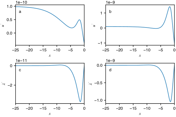
Figure 4: Perturbation profiles for $q=4$ recorded at time $t=50$: a-b) perturbations of velocity $u^{\prime}$, c-d) perturbations of reaction progress variable $\lambda^{\prime}$. Subfigures a) and c) are for $\theta=0.92$ and subfigures b) and d) are for $\theta=0.95$.

5.2.2 Comparison with normal-mode analysis

To check the validity of our computations, we also investigate the system via the normal-mode analysis [27]. The governing equations are linearized about the ZND solution and normal-mode expansions are assumed for the unknowns, $\bm{z}(x,t)=\bar{\bm{z}}\left(x\right)+\epsilon\bm{z}^{\prime}(x)\exp\left(\alpha t\right)$, $D(t)=\bar{D}+\epsilon\psi(t),$ where $\left|\epsilon\right|\ll 1$, $\psi(t)=\exp\left(\alpha t\right)$ is proportional to the perturbation of the unsteady shock relative to its steady-state position, $x(t)=\bar{D}t$, and $\alpha$ is the complex growth rate which is the eigenvalue of the problem. A boundary-value problem is then posed for $\bm{z}^{\prime}(x)$ with the Rankine–Hugoniot conditions on the right boundary (on the shock) and a boundedness condition on the left boundary (at the chemical equilibrium). Substitution of the normal-mode expansions into the governing equations leads to a linearized system for perturbations $\bm{z}^{\prime}$:

$$\alpha\bm{z}^{\prime}+\bm{A}(\bar{\bm{z}})\frac{d\bm{z}^{\prime}}{dx}+\bm{C}\left(\bar{\bm{z}}\right)\bm{z}^{\prime}-\alpha\bm{b}=0,$$

where

$$\bm{A}(\bar{\bm{z}})=\begin{bmatrix}\bar{u}-\bar{D}&\sigma\\ 0&-\bar{D}\end{bmatrix},\quad\bm{C}\left(\bar{\bm{z}}\right)=\begin{bmatrix}\frac{d\bar{u}}{dx}&0\\ -\bar{\omega}_{u}&-\bar{\omega}_{\lambda}\end{bmatrix},\quad\bm{b}=\begin{bmatrix}\frac{d\bar{u}}{dx}\\ \frac{d\bar{\lambda}}{dx}\end{bmatrix}$$

with $\alpha\in\mathbb{C}$, $\bm{z}^{\prime}(x,t)\in\mathbb{C}^{2}$. We reformulate the problem in terms of the steady-state reaction progress variable $\bar{\lambda}$ instead of $x$ using (18) and arrive at the system

$$\frac{d\bm{z}^{\prime}}{d\bar{\lambda}}=-\frac{\bar{D}}{\bar{\omega}}\bm{A}^{-1}\left[-\left(\alpha\bm{I}+\bm{C}\right)\bm{z}^{\prime}+\alpha\bm{b}\right]$$ (45)

which is subject to the linearized Rankine–Hugoniot conditions at $\bar{\lambda}=0$,

$$u^{\prime}=2\alpha,\quad\lambda^{\prime}=0.$$ (46)

The boundedness condition at $x\to-\infty$ is required which expresses the fact that eigenfunctions of the problem must remain bounded at the end of the reaction zone. In [41], a strategy is explained for the derivation of the boundedness condition through the linearization of the forward characteristic equation. Application of this strategy to our model yields

$$H(\alpha)=\alpha\left(\bar{u}u^{\prime}+\sigma\lambda^{\prime}\right)-\sigma\bar{\omega}_{\lambda}\lambda^{\prime}=0,$$ (47)

where $H$ denotes the boundedness function. Thus the problem is reduced to the boundary-value problem (45–47) which has a bounded solution only for particular values of $\alpha$, to be determined. The strategy of solving the problem is based on the shooting method. Namely, (45–46) is solved starting at the shock and integrating toward the end of the reaction zone, where condition (47) must be satisfied. Solving multiple initial-value problems for a range of $\alpha$ allows to plot a “carpet” of $\log(1+|H|)$, in which local minima can be identified that correspond to approximate locations of $\alpha$ that satisfy the boundary-value problem (45–47). Figure 5 shows such a plot for $q=4$, $\theta=0.95$ for the range $\alpha_{\text{re}}\in\{0,0.001,0.002,\dots,0.05\}$, $\alpha_{\text{im}}\in\{0,0.01,0.02,\dots,1]$ with the only local minimum found, which is indicated by a red dot with coordinates $(0.029,0.87)$.

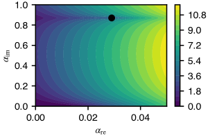
Figure 5: The carpet plot of $\log(1+|H|)$, where $H$ is the boundedness function (47) for $q=4$, $\theta=0.95$. Dot $\left(0.029,0.87\right)$ denotes an approximate local minimum of $\log(1+|H|)$.

Subsequently, using the approximated value of $\alpha$ as an initial guess, we employ a root solver to accurately compute $\alpha$ that satisfies (47). For this, fsolve routine of scipy package is used [23]. The results are shown in Table 1 along with the results found with the method described in Subsection 5.1. Excellent agreement between the two approaches is seen, as growth rates $\alpha_{\text{re}}$ and frequencies $\alpha_{\text{im}}$ match to four and six significant digits, respectively.

Approach	$\alpha_{\text{re}}$	$\alpha_{\text{im}}$
Linear unsteady analysis	0.02909342	0.87041209
Normal-mode analysis	0.02909286	0.87041272

Table 1: Comparison of the growth rates $\alpha_{\text{re}}$ and frequencies $\alpha_{\text{im}}$ of perturbations obtained via linear unsteady computations and normal-mode computations for $q=4$, $\theta=0.95$.

5.2.3 Migration of the linear spectrum as activation energy is varied

Figure 6 shows how the linear spectrum changes as the activation energy, $\theta$, increases in the range $[0.90;1.15]$ with step $\Delta\theta=0.001$. Only one mode in the spectrum is found. Its growth rate increases from $-0.081$ to $0.493$ almost linearly with $\theta$ and a bifurcation to instability occurs at $\theta_{\text{crit}}=0.937\pm 0.001$. The frequency of the mode exhibits slightly more complicated behavior: it initially increases from 0.864 at $\theta=0.90$, reaches the maximum value $0.870$ at $\theta=0.95$, then decreases to $0.738$ at $\theta=1.15$.

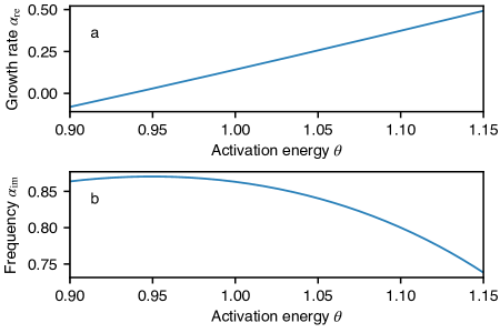
Figure 6: Migration of the linear spectrum for $q=4$ as activation energy $\theta$ is varied: a) growth rate, b) frequency. Each curve consists of 251 points. Only one mode in the spectrum was found.

5.2.4 Neutral stability

Now we turn our attention to the determination of the neutral stability boundary for a wide range of parameters $\theta$ and $q$, that is, the curve in a $\left(\theta,q\right)$ plane that separates stable steady-state solutions from unstable ones. The boundary is determined numerically. For this purpose, we generate 256 linearly spaced values of $q$ in the range $[0.81,16]$ (corresponds to $\bar{D}$ in the range $[0.9,4]$) and for each $q$, we find the critical value of $\theta$ such that the growth rate of instability is close to zero with a tolerance $10^{-3}$. Finding $\theta_{\text{crit}}$ is based on the idea of bisection where a range of $\theta$ is recursively divided in subranges unless the above condition on the growth rate is satisfied. Initial interval of search for $\theta$ is taken $[0.2;5]$. Grid resolution used here is $N_{1/2}=40$.

Figure 7 shows the computed neutral stability curve in the $\left(\theta,q\right)$ plane and the frequency of oscillation $\alpha_{\text{im}}$ along the curve. The data demonstrate that when $q$ increases, $\theta_{\text{crit}}$ decreases while $\alpha_{\text{im}}$ increases. For the lowest $q$ considered here ($q=0.81$), $\theta_{\text{crit}}=4.625$ and $\alpha_{\text{im}}=0.391$, and for the largest $q$ ($q=16$), $\theta_{\text{crit}}\approx 0.234$ and $\alpha_{\text{im}}=1.74$.

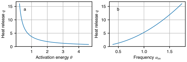
Figure 7: Neutral stability for the Fickett model: a) neutral stability curve in $(\theta,q)$ plane; b) frequency of oscillation $\alpha_{\text{im}}$ along the neutral stability curve. Each curve consists of 256 uniformly spaced points for $q\in[0.81;16]$.

We also provide information about the critical values of activation energy $\theta_{\text{crit}}$ and the frequency of oscillation $\alpha_{\text{im}}$ on the neutral stability boundary for several values of $q$ in Table 2. It is interesting to note that the $(\theta,q)$ neutral curve is nearly a hyperbola, $q\theta\approx 3.75$.

Table 2: Critical values of activation energy $\theta_{\text{crit}}$ and the frequency of oscillation $\alpha_{\text{im}}$ on the neutral stability boundary for several values of heat release $q$.

$i$	$q$	$\theta_{\text{crit}}$	$\alpha_{\text{im}}$
1	$0.81$	4.625	0.391
2	$1.00$	3.746	0.435
3	$2.00$	1.873	0.615
4	$4.00$	0.937	0.870
5	$9.00$	0.417	1.305
6	$16.00$	0.234	1.740

6 Nonlinear dynamics

6.1 Description of the numerical algorithm

Having studied the linear stability properties of the traveling-wave solution and having identified the transition to instability when $\theta q$ is large enough (larger than approximately $3.75$), we now turn attention to the question of the nonlinear dynamics of solutions as we move away from the neutral curve into the unstable domain. To solve the nonlinear system numerically, we use a second-order MUSCL scheme with the minmod flux limiter [29], which we describe below along with the algorithm for the solution of the Riemann problem required for this method.

The MUSCL scheme is a conservative Godunov-type method for a hyperbolic system:

$$\bm{z}_{t}+\bm{f}(\bm{z})_{x}=\bm{s}(\bm{z})$$ (48)

with $\bm{z}\in\mathbb{R}^{n}$ being the vector of unknowns,$\bm{f}:\mathbb{R}^{n}\to\mathbb{R}^{n}$ the flux function, and $\bm{s}$ the source term. Partitioning a computational domain into cells $[x_{i-1/2},x_{i+1/2}]$ (the sketch of the grid is shown in Figure 2b) we obtain a semi-discretized scheme:

$$\frac{d\bar{\bm{z}}_{i}}{dt}=-\frac{\Delta t}{\Delta x}\left(\bm{f}_{i+1/2}-\bm{f}_{i-1/2}\right)+\bm{s}(\bar{\bm{z}}_{i}),$$ (49)

where $\bar{\bm{z}}_{i}$ is the average value of $\bm{z}$ for the computational cell centered at $x_{i}$, and the fluxes at the cell boundaries $\bm{f}_{i+1/2}$ are approximated by reconstructing $\bm{z}_{i+1/2}$. The reconstruction is done through the solution of the Riemann problem with initial conditions

$$\bm{z}_{i+1/2}=\begin{cases}\bm{z}_{\text{L}}&x<x_{i+1/2},\\ \bm{z}_{\text{R}},&x>x_{i+1/2},\end{cases}$$ (50)

where $\bm{z}_{\text{L}}$ and $\bm{z}_{\text{R}}$ are given immediately on the left and the right of $x_{i+1/2}$, respectively. For a second-order scheme, they are found by assuming linear distribution of $\bm{z}_{i}(x)$ in the cell $[x_{i-1/2};x_{i+1/2}]$:

$$\bm{z}_{i}(x)=\bar{\bm{z}}_{i}+\bm{\sigma}_{i}(x-x_{i}),$$ (51)

where $\bm{\sigma}_{i}$ is the slope of the linear reconstruction, therefore,

$$\bm{z}_{\text{L}} =\bar{\bm{z}}_{i}+\bm{\sigma}_{i}\frac{\Delta x}{2},$$ (52)

$$\bm{z}_{\text{R}} =\bar{\bm{z}}_{i+1}-\bm{\sigma}_{i+1}\frac{\Delta x}{2}.$$ (53)

For the second-order MUSCL schemes, $\bm{\sigma}_{i}=\bm{\sigma}_{i}\left(\bar{\bm{z}}_{i}-\bar{\bm{z}}_{i-1},\bar{\bm{z}}_{i+1}-\bar{\bm{z}}_{i}\right)$. We compute $\bm{\sigma}_{i}$ using the minmod flux limiter [29] given componentwise as:

$$\bm{\sigma}_{i}(a,b)=\begin{cases}\min(a,b)/\Delta x,&\text{if }a>0,b>0,\\ \max(a,b)/\Delta x,&\text{if }a<0,b<0,\\ 0,&\text{if }ab<0.\end{cases}$$ (54)

For the model under consideration, solution $\bm{z}_{i+1/2}$ of the Riemann problem corresponds to the state $\left(u_{i+1/2},\lambda_{i+1/2}\right)^{\mathrm{T}}$, which is found by the analysis of the waves that can occur in the Riemann problem and is given in the next subsection. This solution propagates along the line $\left(x_{i+1/2},t\right)^{\mathrm{T}}$ in the $\left(x,t\right)$ plane. As each Riemann problem assumes $x_{i+1/2}=0$ in a local reference frame, the solution is time-independent.

Once all the local Riemann problems are solved over the whole grid, fluxes $\bm{f}_{i+1/2}$ at the edges $x_{i+1/2}$ can be computed. On the left part of the domain, we introduce a ghost point with extrapolation $u_{-1}=u_{0}$ such that the left-most flux $\bm{f}_{-1/2}$ can be computed. On the right boundary the flux $\bm{f}_{N+1/2}$ is computed by means of the Rankine–Hugoniot conditions $u_{N+1/2}=2D$, $\lambda_{N+1/2}=0$, which leads to the fluxes $\bm{f}_{N+1/2}=0$ both for $u$ and $\lambda$ for the chosen ambient conditions.

The time integrator is an adaptive-step Runge–Kutta integrator DOPRI5 [19] as used for the linear unsteady simulations above. It may appear that strong-stability-preserving Runge–Kutta integrators [18] are more appropriate for the problem at hand as we expect internal shocks to be generated inside the reaction zone. However, for the reactive flow, error estimation and consequently adaptive choice of a time step are crucial components of a time integrator. One cannot rely on the Courant–Friedrichs–Lewy condition [29] in the computations of the time step due to chemical reactions occurring at much smaller time scales than wave propagation. The presence of the adaptive-step DOPRI5 integrator in the numerical environment that we use (scipy library of the scientific Python stack [23]) determined our choice of the time integrator. Relative and absolute tolerances of the DOPRI5 integrator are set to $10^{-8}$ and $10^{-6}$, respectively, for the nonlinear simulations.

6.2 The Riemann problem

Below we provide the solution of the Riemann problem for the model system. To analyze possible wave configurations, we write the (nonreactive) system in the characteristic form:

$$\dot{p} =0 \quad\text{on }\dot{x} =u-D,$$ (55)

$$\dot{\lambda} =0 \quad\text{on }\dot{x} =-D,$$ (56)

and from the characteristic equations themselves we can see that the first wave is nonlinear as the characteristic speed depends on $u$ (and correspondingly on $\lambda$ due to coupling), while the second wave is linear and, therefore, second wave is always a left-going wave with speed $-D$. Now, assuming that $u>0$, it is clear that the first wave is always to the right of the second wave and hence the solution consists of three distinct regions: L-region to the left of the second wave, M-region between the second and the first wave, and R-region to the right of the first wave. Now we consider various possible configurations.

Case 1. $u_{\text{L}}<u_{\text{R}}$, $\lambda_{\text{L}}<\lambda_{\text{R}}$. In this case, from the second characteristic equation it follows that $\lambda$ experiences a jump along the line $x=-Dt$, hence this line is the trajectory of the contact discontinuity moving to the left. Then, for M-region, which is to the right of the contact, we have $\lambda_{\text{M}}=\lambda_{\text{R}}$. The invariant $p$ is conserved along the curves $\dot{x}=u-D$, therefore (due to the jump in $\lambda$) $u$ must jump on the contact:

$$\frac{1}{2}\left(u_{\text{M}}^{2}+q\lambda_{\text{M}}\right)=\frac{1}{2}\left(u_{\text{L}}^{2}+q\lambda_{\text{L}}\right),$$ (57)

from which it follows that

$$u_{\text{M}}=\sqrt{u_{\text{L}}^{2}+q(\lambda_{\text{L}}-\lambda_{\text{M}})}=\sqrt{u_{\text{L}}^{2}+q(\lambda_{\text{L}}-\lambda_{\text{R}})}$$ (58)

and hence $u_{\text{M}}<u_{\text{L}}<u_{\text{R}}$. Therefore, the first wave is a centered rarefaction wave, with constraining characteristics

$$x_{\text{HEAD}}=\left(u_{\text{R}}-D\right)t,\quad x_{\text{TAIL}}=\left(u_{\text{M}}-D\right)t,$$ (59)

with the solution inside the rarefaction wave being $u=x/t+D$, which is found from the integration of $\dot{x}=u-D$ with initial conditions $x=0$, $t=0$.

Case 2. $u_{\text{L}}\geq u_{\text{R}}$, $\lambda_{\text{L}}\geq\lambda_{\text{R}}$. In this case $\lambda_{\text{M}}=\lambda_{\text{R}}$ again and $u_{\text{M}}$ is computed using (58) with $u_{\text{M}}\geq u_{\text{L}}\geq u_{\text{R}}$, that is, the characteristics of the first family from M- and R-regions collide and form a shock wave that propagates with speed

$$s=\frac{u_{\text{R}}+u_{\text{M}}}{2}-D.$$ (60)

Case 3. $u_{\text{L}}<u_{\text{R}}$, $\lambda_{\text{L}}\geq\lambda_{\text{R}}$. In this case $\lambda_{\text{M}}=\lambda_{\text{R}}$ and $u_{\text{M}}$ is found using Eq. (58). Hence, the first wave is either a centered rarefaction wave (if $u_{\text{M}}<u_{\text{R}}$) as in Case 1 or a shock wave (if $u_{\text{M}}\geq u_{\text{R}}$) as in Case 2 while the second wave is a contact discontinuity.

Case 4. $u_{\text{L}}\geq u_{\text{R}}$, $\lambda_{\text{L}}<\lambda_{\text{R}}$. In this case $\lambda_{\text{M}}=\lambda_{\text{R}}$ and $u_{\text{M}}$ is found using formula (58). Then the first wave is either a centered rarefaction or a shock wave depending on whether $u_{\text{M}}<u_{\text{R}}$ or $u_{\text{M}}\geq u_{\text{R}}$, that is, this case is the same as Case 3.

For the Godunov method, we are interested in the solution of the Riemann problem along the trajectory $x=0$ only. Summarizing the cases considered above, we conclude that if $u_{\text{R}}>D$, then $u_{i+1/2}=u_{\text{M}}$, $\lambda_{i+1/2}=\lambda_{\text{M}}$. However, the flow can become supersonic with $u_{\text{R}}<D$, particularly near the left boundary, and then not only contact discontinuity moves to the left, but the rarefaction or shock wave as well. In these cases, the solution of the Riemann problem is $u_{i+1/2}=u_{\text{R}}$, $\lambda_{i+1/2}=\lambda_{\text{R}}$.

To illustrate the complete solutions of the Riemann problem and characteristic trajectories, we provide two examples. For both problems, we take $q=9$, hence $D=\sqrt{q}=3$, $\lambda_{\text{L}}=1$, $\lambda_{\text{R}}=0$, and the final time $t=1$. Figure 8a shows the solution of the Riemann problem for $u_{\text{L}}=4$, $u_{\text{R}}=3$, along with the characteristics. As can be seen, the solution consists of three distinct regions: in the region to the left of the contact discontinuity we have $\left(u_{\text{L}},\lambda_{\text{L}}\right)$, between the contact and the shock the state is $\left(u_{\text{M}}=5,\lambda_{\text{R}}\right)$, and to the right of the shock we have $\left(u_{\text{R}},\lambda_{\text{R}}\right)$. As $u_{\text{R}}=D$, the characteristic equations in the rightmost region are vertical. The shock speed in this case is $s=0.5$.

Figure 8b shows the solution of the Riemann problem for $u_{\text{L}}=4$, $u_{\text{R}}=6$, along with the characteristic plane. In this case, the solution consists of four distinct regions: to the left of the contact discontinuity, $x=-Dt$, the solution is $\left(u_{\text{L}},\lambda_{\text{L}}\right)$, between the contact and the tail of the rarefaction wave, the solution is $\left(u_{\text{M}}=5,\lambda_{\text{R}}\right)$, inside the rarefaction wave, we have $\left(u=x/t+D,\lambda_{\text{R}}\right)$, and to the right of the head of the rarefaction solution, we have $\left(u_{\text{R}},\lambda_{\text{R}}\right)$. The head and tail of the rarefaction wave are determined by the lines $x=\left(u_{\text{R}}-D\right)t$ and $x=\left(u_{\text{M}}-D\right)t$, respectively.

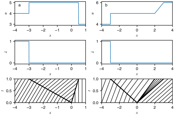
Figure 8: Solution of the Riemann problem and characteristics trajectories up to the final time $t=1$ for $q=9$, $D=3$ and two different initial conditions: a) $\left(u_{\text{L}},\lambda_{\text{L}}\right)=\left(4,1\right)$, $\left(u_{\text{R}},\lambda_{\text{R}}\right)=\left(3,0\right)$; b) $\left(u_{\text{L}},\lambda_{\text{L}}\right)=\left(4,1\right)$, $\left(u_{\text{R}},\lambda_{\text{R}}\right)=\left(6,0\right)$. In both a) and b), bottom plots show the characteristics of the first family, while the characteristics of the second family are not shown except for the trajectory of the contact discontinuity, $x=-Dt$, (all other characteristics of this family are parallel to it).

6.3 Computation of detonation velocity

Now we require an algorithm to evolve $D$ in time. We use a combination of the shock-evolution equation (26) for time steps when the flow is sufficiently smooth and the characteristics-based method from [26] when the flow has steep gradients. Note that in this subsection, subscript “s” is used for the staggered grid point index $N+1/2$ for clarity.

At each time step, we estimate the velocity gradient $du/dx$ using backward finite differences:

$$\left.\frac{du}{dx}\right|_{x_{i}}=\frac{u_{i}-u_{i-1}}{\Delta x},$$ (61)

and if $\|du/dx\|_{\infty}\leq 10$, then the flow is considered smooth. Otherwise, it is considered not smooth.

For smooth flow, we integrate the shock-evolution equation (26) in time simultaneously with (12–13), approximating the velocity gradient appearing in (26) based on the following second-order approximation on the stencil $\{x_{N-1},x_{N},x_{\mathrm{s}}\}$:

$$\left.\frac{du}{dx}\right|_{\mathrm{s}}^{j}=\frac{u_{N-1}^{j}-9u_{N}^{j}+8u_{\mathrm{s}}^{j}}{3\Delta x}$$ (62)

with $u_{\mathrm{s}}^{j}=2D^{j}$ by the Rankine–Hugoniot conditions. Additionally, we set the CFL number to $0.4$.

For non-smooth flow, we use the method from [26] slightly modifying it due to the use of a staggered grid in the present computations. In this method, $D^{j+1}$ is computed using the forward-going characteristic equation and then equations (12–13) are integrated in time; details of the algorithm are given below. CFL number is set to 0.1 in this case.

The forward-going characteristic equation is

$$u\dot{u}+\sigma\dot{\lambda}-\sigma\omega(u,\lambda)=0$$ (63)

satisfied along the trajectory

$$\dot{x}=u-D.$$ (64)

At the time step $j+1$ we are given $u_{i}^{j}$, $\lambda_{i}^{j}$, and $D^{j}$ for $i=0,\dots,N$ and aim to find $D^{j+1}$. We assume that during time step $\Delta t$ from $t^{j}$ to $t^{j+1}$, characteristics are straight lines and then approximate the trajectory of the characteristic that starts at location $x_{*}^{j}$ at time $t^{j}$ and arrives to the shock $x_{\mathrm{s}}=0$ at time $t^{j+1}$ using the forward Euler method:

$$x_{\mathrm{s}}-x_{*}^{j}=\left(u_{*}^{j}-D^{j}\right)\Delta t,$$ (65)

where $u_{*}^{j}=u(x_{*}^{j},t^{j})$ and $x_{\mathrm{s}}=0$ for any time step. To find $u_{*}^{j}$, we interpolate linearly using the value at the shock and the given average of $u_{N}^{j}$ in the rightmost computational cell:

$$\frac{u_{\mathrm{s}}^{j}-u_{N}^{j}}{x_{\mathrm{s}}-x_{N}}=\frac{u_{*}^{j}-u_{N}^{j}}{x_{*}-x_{N}}.$$ (66)

Using relations $x_{\mathrm{s}}-x_{N}=\Delta x/2$ and $x_{N}=-\Delta x/2$, we arrive at the following formula for $u_{*}^{j}$:

$$u_{*}^{j}=u_{\mathrm{s}}^{j}+\frac{2\left(u_{\mathrm{s}}^{j}-u_{N}^{j}\right)}{\Delta x}x_{*},$$ (67)

with $u_{\mathrm{s}}^{j}=2D^{j}$. Similarly, we obtain the formula for $\lambda_{*}^{j}$:

$$\lambda_{*}^{j}=\lambda_{\mathrm{s}}^{j}+\frac{2\left(\lambda_{\mathrm{s}}^{j}-\lambda_{N}^{j}\right)}{\Delta x}x_{*}$$ (68)

with $\lambda_{\mathrm{s}}^{j}=0$.

Now, by substituting expression for $u_{*}^{j}$ into (65), we find that $x_{*}^{j}$ can be computed explicitly:

$$x_{*}^{j}=\frac{D^{j}\Delta t}{-1-\frac{2\left(u_{\mathrm{s}}^{j}-u_{N}^{j}\right)}{\Delta x}}.$$ (69)

After computing $x_{*}^{j}$, $u_{*}^{j}$, and $\lambda_{*}^{j}$, the updated detonation velocity, $D^{j+1}$, is found by solving a nonlinear equation arising from the discretization of (63):

$$u_{*}^{j}\frac{u_{\mathrm{s}}^{j+1}-u_{*}^{j}}{\Delta t}+\sigma\frac{\lambda_{\mathrm{s}}^{j+1}-\lambda_{*}^{j}}{\Delta t}-\sigma\omega\left(u_{\mathrm{s}}^{j+1},\lambda_{\mathrm{s}}^{j+1}\right)=0,\text{ where }u_{\mathrm{s}}^{j+1}=2D^{j+1},\quad\lambda_{\mathrm{s}}^{j+1}=0,$$ (70)

which is done using the Newton method with the termination condition that the relative error in $D^{j+1}$ between two subsequent iterations is less than $10^{-8}$.

6.4 Bifurcation diagram

Now we turn our attention to various solutions of the model when the activation energy $\theta$ is increased while other parameters are kept fixed. For some values of $\theta$, the solution is found to undergo bifurcations from one nonlinear regime to another. To visualize these bifurcations, we run simulations for $\theta\in[0.90;1.15]$ with step $0.001$ up to time $T_{\text{final}}=1000$ and in each simulation we extract local minima of the time series of detonation velocity, $D(t)$, for time window $t\in[900;1000]$; subsequently, the minima are plotted against $\theta$ on a bifurcation diagram. Each simulation is conducted using $q=4$, $\text{tol}_{\lambda}=10^{-6}$, and $N_{1/2}=1280$ with an initial condition being the corresponding ZND solution. Then, necessary perturbation of the initial condition is supplied by the truncation error of the numerical scheme.

Figure 9 shows the resultant bifurcation diagram. Note its resemblance of the well-known diagram for the logistic map in the sense that, as $\theta$ increases, solution undergoes a series of period-doubling bifurcations until eventually chaotic-looking regimes appear. Similar diagrams have also been found previously in various models of detonation [33, 20, 35, 25, 11].

In Figure 9 at $\theta\in[0.9;0.936]$, the solution is asymptotically stable as the initial perturbation decays with $D\to D_{\text{CJ}}$ as $t\to\infty$; at $\theta=0.937$ a bifurcation takes place from a stable steady-state solution to a period-1 stable limit cycle, and then the solution stays qualitatively the same for $\theta\in[0.937,1.001]$ with the local minima decreasing below $D_{\text{CJ}}$ value; at $\theta=1.002$ the second bifurcation occurs to a period-2 limit cycle, and then the cycle is preserved for $\theta\in[1.002;1.056]$ with the top minima increasing and bottom minima decreasing; at $\theta=1.074$ the solution bifurcates to a period-4 limit cycle. For larger $\theta$ ($\theta\gtrapprox 1.077$), the solution is appearing to be chaotic as a large number of minima are found. However, for $\theta\in\{1.089,1.09\}$ period-6 limit cycle is obtained.

It must be mentioned that at $\theta\gtrapprox 1.077$, it becomes quite challenging to compute the solutions sufficiently accurately due to internal shocks appearing and hitting the lead shock, effectively making the reaction zone unresolved even for resolution $N_{1/2}=1280$ that is used for these computations. We also run the simulations with twice and four times coarser grids to verify the convergence of the bifurcation diagram for stable limit cycles for $\theta\lessapprox 1.077$.

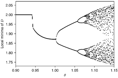
Figure 9: Bifurcation diagram for $q=4$, $\theta\in[0.95;1.15]$ with step $\Delta\theta=0.001$.

6.5 Stable limit cycles

Now we consider time series for several different values of $\theta$ that correspond to qualitatively different nonlinear dynamics as evident from the bifurcation diagram 9. We also plot phase portraits in $\dot{D}-D$ plane to better understand the dynamics. The shock acceleration $\dot{D}$ is approximated by central finite differences:

$$\dot{D}=\frac{D_{i+1}-D_{i-1}}{t_{i+1}-t_{i-1}}\text{ for }i=1,2,\dots,$$ (71)

and initial acceleration is taken to be zero, $\dot{D}\left(0\right)=0$. As time series contain numerical noise, to regularize numerical differentiation, the $D\left(t\right)$ series are first smoothed using the simple moving average algorithm with window size 11, and after obtaining $\dot{D}$ using (71), it is also smoothed using the same algorithm with window size 5.

Figures 10a,b show the nonlinear dynamics for $\theta=0.95$ and $\theta=1$, which is a stable limit cycle in these two cases. Figures 10c,d demonstrate period-2 limit cycles for $\theta=1.004$ and $\theta=1.055$, respectively. From these figures we can see that as $\theta$ increases, distance between top and bottom minima increases as well: for $\theta=1.004$, the ratio of relative minima is $\approx 1.11$, while for $\theta=1.055$, this ratio is $\approx 1.84$. Figures 10e,f show period-4 nonlinear oscillations for $\theta=1.065$ and period-6 nonlinear oscillations for $\theta=1.089$. It can be also noticed that as $\theta$ increases, the range of detonation acceleration $\dot{D}$ increases dramatically: for weakly unstable cases $\dot{D}$ is in the order of unity, while for strongly unstable cases, it is in the order of 1000 as can be seen from Figures 10d-f.

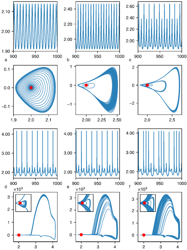
Figure 10: The time series and phase portraits of nonlinear solutions for $q=4$ and various $\theta$: (a) $\theta=0.95$, (b) $\theta=1$, (c) $\theta=1.004$, (d) $\theta=1.055$, (e) $\theta=1.065$, (f) $\theta=1.089$. Plots in the odd rows show time series $D$ versus $t$, while plots in the even rows show corresponding phase portraits $\dot{D}$ versus $D$. Insets in the bottom row have limits $(1.8,2.5)$ on the $x$-axis and $(-1,1)$ on the $y$-axis.

7 Code verification

In this section, we assess the correctness of our linear and nonlinear solvers. It is widely accepted [39, 38] that the most stringent test case is the comparison of the observable order of accuracy with theoretical order of accuracy of the numerical methods used to discretize the governing equations. For all convergence studies below, we compute the observed order of accuracy by the following procedure. Let the convergence study to be performed with $N$ grid resolutions. Then the order of accuracy is

$$r_{i}=\frac{\log\left(E_{i}/E_{i-1}\right)}{\log\left(\Delta x_{i}/\Delta x_{i-1}\right)},\quad i=3,\dots,N,$$ (72)

where $E_{i}$ is an error for the $i$-th resolution and $\Delta x_{i}$ is a spatial step for the $i$-th grid resolution.

7.1 Convergence study

We test the linear solver as follows. Simulations are run for $q=4$ and $\theta=1$ with several grid resolutions, and relative errors are computed as

$$E_{i}=\frac{\|\psi^{\prime}_{i}-\psi^{\prime}_{i-1}\|}{\|\psi^{\prime}_{i}\|},\quad i=2,\dots,N,$$ (73)

where $\psi^{\prime}_{i}$ is the time series of the perturbation of detonation velocity obtained with $i$-th grid resolution, $N$ is the total number of resolutions, and norms are $L_{1}$, $L_{2}$, and $L_{\infty}$. If the observed order of accuracy (72) matches the theoretical fifth order, then one concludes that the implementation of the solver is correct.

Table 3 shows the obtained errors and orders of accuracy for the linear solvers where errors were computed with different norms. It can be seen that the observed order of accuracy is five, hence, the implementation of the linear solver is correct. The sudden drop of the order of accuracy for the resolution $N_{1/2}=1280$ is due to the domination of the rounding errors of the floating-point arithmetic over the truncation errors of the numerical schemes at this resolution.

Table 3: Convergence study for the linear solver for $q=4$, $\theta=1$. $N_{1/2}$ is the resolution per half-reaction zone, $E_{1}$, $E_{2}$, $E_{\infty}$ are relative errors computed by (73) in $L_{1}$, $L_{2}$, and $L_{\infty}$ norms, respectively; $r_{1}$, $r_{2}$, $r_{\infty}$ are corresponding observed orders of accuracy. Negative values for orders of accuracy are due to the domination of the round-off error of floating-point arithmetic over truncation error of numerical methods used.

$N_{1/2}$	$E_{1}$	$r_{1}$	$E_{2}$	$r_{2}$	$E_{\infty}$	$r_{\infty}$
20	N/A	N/A	N/A	N/A	N/A	N/A
40	$9\text{\times}{10}^{-05}$	N/A	$9\text{\times}{10}^{-05}$	N/A	$1\text{\times}{10}^{-04}$	N/A
80	$3\text{\times}{10}^{-06}$	5.20	$3\text{\times}{10}^{-06}$	5.20	$3\text{\times}{10}^{-06}$	5.19
160	$8\text{\times}{10}^{-08}$	5.10	$8\text{\times}{10}^{-08}$	5.10	$8\text{\times}{10}^{-08}$	5.10
320	$2\text{\times}{10}^{-09}$	5.06	$2\text{\times}{10}^{-09}$	5.06	$3\text{\times}{10}^{-09}$	5.06
640	$6\text{\times}{10}^{-11}$	5.42	$7\text{\times}{10}^{-11}$	5.25	$3\text{\times}{10}^{-10}$	3.13
1280	$6\text{\times}{10}^{-11}$	-0.10	$7\text{\times}{10}^{-11}$	-0.05	$4\text{\times}{10}^{-10}$	-0.49

For the nonlinear solver, we compute the solution on several different grids for $q=4$, $\theta=0.92$. For these parameters, the solution is stable, hence, $D\to D_{\text{CJ}}$ at large times. Here we take $T_{\text{final}}=300$. We do not specify any perturbation in this case, so that the perturbation of the initial traveling-wave solution is only due to the truncation error of the scheme. The global error is then defined by

$$E_{i}=\|D_{i}(t)-D_{\text{CJ}}\|_{2}\text{ for }i=1,\dots,N,$$

where $D_{i}(t)$ is the time series of detonation velocity for the $i$-th grid resolution, and the norm is $L_{2}$-norm. Then the observed order of accuracy is computed using (72). Table 4 shows the obtained errors and the orders of accuracy. It can be seen that the order of accuracy matches the theoretical second order which confirms that the nonlinear solver described in Subsection 6.2 is implemented correctly and is second-order accurate at least for the stable flows.

Table 4: Convergence study for the nonlinear solver using parameters $q=4$, $\theta=0.92$, $T_{\text{final}}=300$.

$N_{1/2}$	$E$	$r$
20	$2\text{\times}{10}^{-04}$	N/A
40	$5\text{\times}{10}^{-05}$	2.11
80	$1\text{\times}{10}^{-05}$	2.05
160	$3\text{\times}{10}^{-06}$	2.01
320	$8\text{\times}{10}^{-07}$	1.99

Additionally, we run a convergence study for the nonlinear solver for the case when the solution is a stable limit cycle with small amplitude of oscillations so that the solver uses only second-order approximations. We run simulations for $q=4$ and $\theta=0.95$ with several grid resolutions and extract local minima from the time series of detonation velocity for $t\in[900;1000]$. For each grid resolution, the average of the local minima $D_{\text{avg min},i}$ is computed. Then the errors are computed by comparing the obtained average to the next average:

$$E_{i}=|D_{\text{avg min},i}-D_{\text{avg min},i+1}|,\quad i=1,\dots N-1,$$ (74)

where $N$ is the number of grid resolutions. Then the order of accuracy is computed using (72). Table 5 displays the obtained errors and orders of accuracy. It can be seen that the observed order of accuracy is two as expected, hence the implementation of the nonlinear solver is correct not only for stable solutions, but also for weakly unstable solutions.

Table 5: Convergence study for the nonlinear solver with parameters $q=4$, $\theta=0.95$.

$N_{1/2}$	$E$	$r$
20	N/A	N/A
40	$2\text{\times}{10}^{-03}$	N/A
80	$5\text{\times}{10}^{-04}$	2.13
160	$1\text{\times}{10}^{-04}$	2.07
320	$3\text{\times}{10}^{-05}$	2.04
640	$7\text{\times}{10}^{-06}$	2.03
1280	$2\text{\times}{10}^{-06}$	2.09

7.2 Comparison of linear and nonlinear solutions

In this subsection, we compare the solutions of the linear and nonlinear problems for further verification. If parameters of the problem are such that the ZND solution is unstable and the initial amplitude of the perturbation of the solution is small relative to the ZND solution itself, then for early times both linear and nonlinear solutions should agree with each other.

Figure 11 shows detonation velocity as a function of time obtained both from linear and nonlinear solvers for heat release $q=4$ and activation energy $\theta=0.95$, with resolutions $N_{1/2}=40$ and $N_{1/2}=320$ for linear and nonlinear solvers, respectively, and initial perturbation amplitude $A_{0}=10^{-4}$. This choice of resolutions and initial amplitude is dictated by the difference in the order of accuracy of the solvers (fifth for linear and second for nonlinear). In Figure 11a, the detonation velocity is shown at early times, when the amplitude of the perturbation is small. As we can see, the solutions of the linear and nonlinear problems are indistinguishable from each other: they both exhibit exponential growth with the same frequency of oscillations. In Figure 11b, the detonation velocity is shown at later times when the amplitude of the perturbation becomes comparable with $D_{\text{CJ}}$. It can be seen that the linear solution continues to grow exponentially while the nonlinear solution saturates on a limit cycle. The agreement of the two solutions at early times additionally verifies the correctness of both linear and nonlinear solvers.

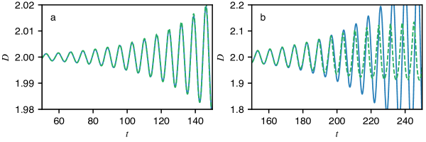
Figure 11: Comparison of solutions of linearized (solid line) and nonlinear (dashed line) problems: a) at early times when the amplitude of perturbation is small comparing to $D_{\mathrm{CJ}}=2$ and two solutions are indistinguishable; b) at later times when the amplitude of perturbation is large and two solutions diverge: linear solution continues to grow exponentially while the nonlinear solution exhibits a limit cycle.

8 Conclusions

In this work, we carried out a comprehensive numerical investigation of the linear and nonlinear dynamics of solutions of a relatively simple $2\times 2$ system of hyperbolic balance laws that possesses nontrivial dynamical properties. It is demonstrated that traveling-wave solutions of the system can become unstable as a system parameter is varied. As a result of the instability, the solutions tend asymptotically in time to a limit cycle attractor of varying complexity. Stable periodic limit cycles as well as what appears to be a chaotic attractor are found in the simulations.

The numerical predictions are verified extensively by convergence studies and comparisons of results obtained by different numerical algorithms. The linear stability of traveling shock-wave solutions is computed by a shock-fitting method which is fifth-order in space and time using the direct method of [24]. These results are compared with those computed by the method of normal modes, and complete agreement is found. The nonlinear simulations are performed using the second-order Godunov method implemented also in a shock-fitting approach. Convergence tests and comparisons with linear predictions when appropriate verify the accuracy of the computed results and confirm the presence of limit cycles, period-doubling bifurcations, and possible chaos in this simple hyperbolic system.

Extensions of the present work that are of theoretical interest include problems involving additional factors, such as diffusive effects, and understanding their role in the nature of the periodic and chaotic solutions of the system.

Supplementary Materials

The datasets and the scripts reproducing the figures and tables in this work are available at https://doi.org/10.5281/zenodo.1297175.

References

- Bdzil and Stewart [2007] Bdzil, J. B., Stewart, D. S., 2007. The dynamics of detonation in explosive systems. Annu. Rev. Fluid Mech. 39, 263–292.
- Bdzil and Stewart [2012] Bdzil, J. B., Stewart, D. S., 2012. Theory of detonation shock dynamics. In: Shock Waves Science and Technology Library, Vol. 6. Springer, pp. 373–453.
- Brown et al. [1989] Brown, P. N., Byrne, G. D., Hindmarsh, A. C., 1989. VODE: A variable-coefficient ODE solver. SIAM journal on scientific and statistical computing 10 (5), 1038–1051.
- Chen and Gurtin [1971] Chen, P., Gurtin, M., 1971. Growth and decay of one-dimensional shock waves in fluids with internal state variables. Physics of Fluids 14 (6), 1091–1094.
-
Clavin [2017]
Clavin, P., 2017. Nonlinear dynamics of shock and detonation waves in gases.
Combustion Science and Technology 189 (5), 747–775.
URL http://dx.doi.org/10.1080/00102202.2016.1260562 - Clavin and Williams [2002] Clavin, P., Williams, F. A., 2002. Dynamics of planar gaseous detonations near Chapman-Jouguet conditions for small heat release. Combustion Theory and Modelling 6 (1), 127–139.
- Clavin and Williams [2012] Clavin, P., Williams, F. A., 2012. Analytical studies of the dynamics of gaseous detonations. Philosophical Transactions of the Royal Society A: Mathematical, Physical and Engineering Sciences 370 (1960), 597–624.
- Döring [1943] Döring, W., 1943. Uber den detonationvorgang in gasen. Annalen der Physik 43(6/7), 421–428.
-
Faria and Kasimov [2015]
Faria, L. M., Kasimov, A. R., 2015. Qualitative modeling of the dynamics of
detonations with losses. Proceedings of the Combustion Institute 35,
2015–2023.
URL http://www.sciencedirect.com/science/article/pii/S1540748914003162 -
Faria et al. [2014]
Faria, L. M., Kasimov, A. R., Rosales, R. R., 2014. Study of a model equation
in detonation theory. SIAM Journal on Applied Mathematics 74 (2), 547–570.
URL http://epubs.siam.org/doi/abs/10.1137/130938232 - Faria et al. [2015] Faria, L. M., Kasimov, A. R., Rosales, R. R., 2015. Theory of weakly nonlinear self-sustained detonations. Journal of Fluid Mechanics 784, 163–198.
- Faria et al. [2016] Faria, L. M., Kasimov, A. R., Rosales, R. R., 2016. Study of a model equation in detonation theory: multidimensional effects. SIAM J. Appl. Maths 76 (3), 887–909.
-
Fickett [1979]
Fickett, W., 1979. Detonation in miniature. American Journal of Physics
47 (12), 1050–1059.
URL http://link.aip.org/link/?AJP/47/1050/1 - Fickett [1984] Fickett, W., 1984. Shock initiation of detonation in a dilute explosive. Physics of Fluids 27, 94.
- Fickett [1985a] Fickett, W., 1985a. Introduction to Detonation Theory. University of California Press, Berkeley, CA.
- Fickett [1985b] Fickett, W., 1985b. Stability of the square-wave detonation in a model system. Physica D: Nonlinear Phenomena 16 (3), 358–370.
- Fickett and Davis [2011] Fickett, W., Davis, W. C., 2011. Detonation: theory and experiment. Dover Publications.
- Gottlieb et al. [2001] Gottlieb, S., Shu, C., Tadmor, E., 2001. Strong stability-preserving high-order time discretization methods. SIAM review, 89–112.
- Hairer et al. [1993] Hairer, E., Nørsett, S. P., Wanner, G., 1993. Solving Ordinary Differential Equations I: Nonstiff problems. Springer.
- Henrick et al. [2006] Henrick, A. K., Aslam, T. D., Powers, J. M., 2006. Simulations of pulsating one-dimensional detonations with true fifth order accuracy. J. Comput. Phys. 213 (1), 311–329.
- Humpherys et al. [2013] Humpherys, J., Lyng, G., Zumbrun, K., 2013. Stability of viscous detonations for Majda’s model. Physica D: Nonlinear Phenomena 259, 63–80.
- Humpherys and Zumbrun [2010] Humpherys, J., Zumbrun, K., 2010. Efficient numerical stability analysis of detonation waves in ZND. arXiv preprint arXiv:1011.0897.
-
Jones et al. [2001–]
Jones, E., Oliphant, T., Peterson, P., et al., 2001–. SciPy: Open source
scientific tools for Python.
URL http://www.scipy.org/ - Kabanov and Kasimov [2018] Kabanov, D. I., Kasimov, A. R., 2018. Linear stability analysis of detonations via numerical computation and dynamic mode decomposition. Physics of Fluids 30 (3), 036103.
- Kasimov et al. [2013] Kasimov, A. R., Faria, L. M., Rosales, R. R., 2013. Model for shock wave chaos. Physical Review Letters 110 (10), 104104.
- Kasimov and Stewart [2004] Kasimov, A. R., Stewart, D. S., 2004. On the dynamics of self-sustained one-dimensional detonations: A numerical study in the shock-attached frame. Physics of Fluids 16, 3566.
- Lee and Stewart [1990] Lee, H. I., Stewart, D. S., 1990. Calculation of linear detonation instability: One-dimensional instability of plane detonation. J. Fluid Mech. 212, 103–132.
- LeVeque [1992] LeVeque, R., 1992. Numerical methods for conservation laws. Birkhäuser.
- LeVeque [2002] LeVeque, R. J., 2002. Finite volume methods for hyperbolic problems. Cambridge University Press.
- Levy [1992] Levy, A., 1992. On Majda’s model for dynamic combustion. Communications in partial differential equations 17 (3-4), 657–698.
- Lyng and Zumbrun [2004] Lyng, G., Zumbrun, K., 2004. A stability index for detonation waves in Majda’s model for reacting flow. Physica D: Nonlinear Phenomena 194 (1), 1–29.
-
Majda [1980]
Majda, A., 1980. A qualitative model for dynamic combustion. SIAM Journal on
Applied Mathematics 41 (1), 70–93.
URL http://link.aip.org/link/?SMM/41/70/1 - Ng et al. [2005] Ng, H., Higgins, A., Kiyanda, C., Radulescu, M., Lee, J., Bates, K., Nikiforakis, N., 2005. Nonlinear dynamics and chaos analysis of one-dimensional pulsating detonations. Combust. Theory Model 9 (1), 159–170.
- Radulescu and Tang [2011] Radulescu, M. I., Tang, J., 2011. Nonlinear dynamics of self-sustained supersonic reaction waves: Fickett’s detonation analogue. Phys. Rev. Lett. 107 (16).
- Romick et al. [2012] Romick, C. M., Aslam, T. D., Powers, J. M., 2012. The effect of diffusion on the dynamics of unsteady detonations. Journal of Fluid Mechanics 699, 453.
- Rosales [1989] Rosales, R. R., 1989. Diffraction effects in weakly nonlinear detonation waves. In: Nonlinear Hyperbolic Problems. Vol. 1402 of Lecture Notes in Mathematics. Springer, pp. 227–239.
- Rosales and Majda [1983] Rosales, R. R., Majda, A. J., 1983. Weakly nonlinear detonation waves. SIAM Journal on Applied Mathematics 43 (5), 1086–1118.
-
Roy [2005]
Roy, C. J., 2005. Review of code and solution verification procedures for
computational simulation. Journal of Computational Physics 205 (1), 131 –
156.
URL http://www.sciencedirect.com/science/article/pii/S0021999104004619 - Salari and Knupp [2000] Salari, K., Knupp, P., 2000. Code verification by the method of manufactured solutions. Tech. rep., Sandia National Labs., Albuquerque, NM (US); Sandia National Labs., Livermore, CA (US).
- Schmid [2010] Schmid, P. J., 2010. Dynamic mode decomposition of numerical and experimental data. Journal of Fluid Mechanics 656, 5–28.
- Stewart and Kasimov [2005] Stewart, D. S., Kasimov, A. R., 2005. Theory of detonation with an embedded sonic locus. SIAM J. Appl. Maths. 66 (2), 384–407.
- Stewart and Kasimov [2006] Stewart, D. S., Kasimov, A. R., 2006. State of detonation stability theory and its application to propulsion. Journal of Propulsion and Power 22 (6), 1230.
- Tang and Radulescu [2012] Tang, J., Radulescu, M., 2012. Dynamics of shock induced ignition in Ficketts model: Influence of . Proceedings of the Combustion Institute.
- Taylor et al. [2009] Taylor, B. D., Kasimov, A. R., Stewart, D. S., 2009. Mode selection in weakly unstable two-dimensional detonations. Combustion Theory and Modelling 13 (6), 973–992.
- Trefethen and Bau III [1997] Trefethen, L. N., Bau III, D., 1997. Numerical linear algebra. Vol. 50. Siam.
- Tu et al. [2014] Tu, J. H., Rowley, C. W., Luchtenburg, D. M., Brunton, S. L., Kutz, J. N., 2014. On dynamic mode decomposition: theory and applications. Journal of Computational Dynamics 1 (2), 391–421.
- von Neumann [1942] von Neumann, J., 1942. Theory of detonation waves. Office of Scientific Research and Development, Report 549. Tech. rep., National Defense Research Committee Div. B.
- Zel’dovich [1940] Zel’dovich, Y. B., 1940. On the theory of propagation of detonation in gaseous systems. J. Exp. Theor. Phys. 10 (5), 542–569.
- Zumbrun [2017] Zumbrun, K., 2017. Recent results on stability of planar detonations. In: Shocks, Singularities and Oscillations in Nonlinear Optics and Fluid Mechanics. Springer, pp. 273–308.