A survey on zeros of random holomorphic sections

Abstract.

We survey results on the distribution of zeros of random polynomials and of random holomorphic sections of line bundles, especially for large classes of probability measures on the spaces of holomorphic sections. We provide furthermore some new examples of measures supported in totally real subsets of the complex probability space.

1. Introduction

The main purpose of this paper is to review some results on the distribution of zeros of random polynomials and more generally of random holomorphic sections of line bundles. A general motivating question is the following. If the coefficients of a polynomial are subject to random error, the zeros of this polynomial will also be subject to random error. It is natural to enquire how the latter errors depend upon the former. One considers therefore polynomials whose coefficients are independent identically distributed random variables and studies the statistical properties of the zeros, such as the number of real zeros and uniformity of the zero distribution. Many classical works are devoted to this circle of ideas: Bloch-Pólya [BP], Littelwood-Offord [LO1, LO2, LO3], Erdős-Turán [ET], Kac [K], Hammersley [H].

The distribution of zeros of polynomials with random coefficients is also relevant for problems which naturally arise in the context of quantum chaotic dynamics or in other domains of physics [BBH, NV]. One can view zeros of polynomials in one complex variable as interacting particles in two dimensions, as, for instance, eigenvalues of random asymmetric matrices can be physically interpreted as a two-dimensional electron gas confined in a disk.

There is an interesting connection between equidistribution of zeros and Quantum Unique Ergodicity related to a conjecture of Rudnik-Sarnak [RS] about the behavior of high energy Laplace eigenfunctions on a Riemannian manifold. By replacing Laplace eigenfunctions with modular forms one is lead to study of the equidistribution of zeros of Hecke modular forms, see Holowinsky-Soundararajan [HS].

The first purpose of this survey is to review some results on asymptotic equilibrium distribution of zeros of polynomials which arose from the work of Bloom [B1, B2] and Bloom-Levenberg [BL]. They pointed out the role of the extremal plurisubharmonic functions in the equidistribution result. Bloom [B1, B2] also introduced the Bernstein-Markov measures as a convenient general framework for defining the Gaussian random sections. A conceptual and very fruitful approach is to introduce an inner product on the space of polynomials which induces the Gaussian probability measure and to consider the asymptotics of the Bergman kernel associated to this inner product [B1, B2, BL, SZ2]. This is generalized in Theorem 2.2 for the weighted global extremal function of a locally regular weighted closed set. We will moreover study the distribution of common zeros of a $k$-tuple of polynomials in Section 2.3 and give a central limit theorem for the linear statistics of the zeros in Section 2.4.

In the second part of the paper we consider random holomorphic sections of line bundles over complex manifolds with respect to weights and measures satisfying some quite weak conditions. Polynomials of degree at most $p$ on $\mathbb{C}$ generalize to the space $H^{0}(X,L^{p})$ of holomorphic sections of the $p$-th power of an ample line bundle $L\to X$ over any complex manifold of dimension $n$. The weight used in the case of polynomials generalizes to a Hermitian metric $h$ on $L$. In the case $h$ is smooth and has positive curvature $\omega=c_{1}(L,h)$, Shiffman-Zelditch [SZ1] showed that the asymptotic equilibrium distribution (see also [NV] for genus one surfaces in dimension one) of zeros of sections in $H^{0}(X,L^{p})$ as $p\to\infty$ is given by the volume form $\omega^{n}/n!$ of the metric. Dinh-Sibony [DS1] introduced another approach, which also gives an estimate of the speed of convergence of zeros to the equilibrium distribution (see also [DMS] for the non-compact setting). This result was generalized for singular metrics whose curvature is a Kähler current in [CM1] and for sequences of line bundles over normal complex spaces in [CMM] (see also [CM2, CM3, DMM]). In Section 3 we review results from [BCM] where we generalize the setting of [CMM] for probability measures satisfying a very general moment condition (see Condition (B) therein), including measures with heavy tail and small ball probability. Important examples are provided by the Guassians and the Fubini-Study volumes.

In Section 4, we provide some new examples of measures that satisfy the moment condition. They have support contained in totally real subsets of the complex probability space.

Finally, in Section 5 we illustrate the equilibrium distribution of zeros by pictures of the zero divisors for the case of polynomials with inner product over the square in the plane and for $SU_{2}$ polynomials.

2. Random Polynomials on $\mathbb{C}^{n}$

In this section we survey some statistical properties of zeros of random polynomials associated with a locally regular set $Y\subset\mathbb{C}^{n}$ and a weight function $\varphi:Y\to\mathbb{R}$. Classical Weyl polynomials arise as a special case. We denote by $\lambda_{2n}$ the Lebesgue measure on $\mathbb{C}^{n}\simeq\mathbb{R}^{2n}$. We also denote by $\mathbb{C}[z]$ the space of polynomials in $n$ complex variables, and we let $\mathbb{C}_{p}[z]=\{f\in\mathbb{C}[z]:\,\deg f\leq p\}$. Recall that $d=\partial+\overline{\partial}$ and $d^{c}:=\frac{i}{2\pi}(\overline{\partial}-\partial)$, so that $dd^{c}=\frac{i}{\pi}\partial\overline{\partial}$.

2.1. Weighted global extremal function

Let $Y\subset\mathbb{C}^{n}$ be a (possibly) unbounded closed set and $\varphi:Y\to\mathbb{R}$ be a continuous function. If $Y$ is unbounded, we assume that there exists $\epsilon>0$ such that

(2.1) $$\varphi(z)\geq(1+\epsilon)\log|z|\ \text{for}\ |z|\gg 1.$$

We note that this framework includes the case when $Y$ is compact and $\varphi:Y\to\mathbb{R}$ is any continuous function. Following [SaT, Appendix B] we introduce the weighted global extremal function,

(2.2) $$V_{Y,\varphi}(z):=\sup\{u(z):u\in\mathcal{L}(\mathbb{C}^{n}),u\leq\varphi\ \text{on}\ Y\}\,,$$

where $\mathcal{L}(\mathbb{C}^{n})$ denotes the Lelong class of plurisubharmonic (psh) functions $u$ that satisfies

$$u(z)-\log^{+}|z|=O(1)$$

where $\log^{+}=\max(\log,0)$. We let

$$\mathcal{L}^{+}(\mathbb{C}^{m}):=\{u\in\mathcal{L}(\mathbb{C}^{m}):u(z)\geq\log^{+}|z|+C_{u}\ \text{for some}\ C_{u}\in\mathbb{R}\}.$$

In what follows, we let

$$g^{*}(z):=\limsup_{w\to z}g(w)$$

denote the upper semi-continuous regularization of $g$. Seminal results of Siciak and Zaharyuta (see [SaT, Appendix B] and references therein) imply that $V^{*}_{Y,\varphi}\in\mathcal{L}^{+}(\mathbb{C}^{m})$ and that $V_{\varphi}$ verifies

(2.3) $$V_{Y,\varphi}(z)=\sup\left\{\frac{1}{\deg f}\,\log|f(z)|:\,f\in\mathbb{C}[z]\,,\;\sup_{z\in Y}|f(z)|e^{-(\deg f)\varphi(z)}\leq 1\right\}.$$

For $r>0$ let us denote

$$Y_{r}:=\{z\in Y:\,|z|\leq r\}\,.$$

Then it follows that $V_{Y,\varphi}=V_{Y_{r},\varphi}$ for sufficiently large $r\gg 1$ ([SaT, Appendix B, Lemma 2.2]).

A closed set $Y\subset\mathbb{C}^{n}$ is said to be locally regular at $w\in Y$ if for every $\rho>0$ the extremal function $V_{Y\cap\overline{B(w,\rho)}}(z)$ is continuous at $w$. The set $Y$ is called locally regular if $Y$ is locally regular at each $w\in Y$. A classical result of Siciak [Si] asserts that of $Y$ is locally regular and $\varphi$ is continuous weight function then the weighted extremal function $V_{Y,\varphi}$ is also continuous and hence $V_{Y,\varphi}=V_{Y,\varphi}^{*}$ on $\mathbb{C}^{n}$. In the rest of this section we assume that $Y$ is a locally regular closed set.

The psh function $V_{Y,\varphi}$ is locally bounded on $\mathbb{C}^{n}$ and hence by the Bedford-Taylor theory [BT1, BT2] the weighted equilibrium measure

$$\mu_{Y,\varphi}:=\frac{1}{n!}(dd^{c}V_{Y,\varphi})^{n}$$

is well-defined and does not put any mass on pluripolar sets. Moreover, if $S_{Y,\varphi}:=\operatorname{supp}\mu_{Y,\varphi}$ then by [SaT, Appendix B] we have $S_{Y,\varphi}\subset\{V_{Y,\varphi}=\varphi\}$. Hence, the support $S_{Y,\varphi}$ is a compact set. An important example is $Y=\mathbb{C}^{n}$ and $\varphi(z)=\frac{\|z\|^{2}}{2}$, which gives $\mu_{Y,\varphi}=\mathbbm{1}_{B}\,d\lambda_{2n}(z)$, where $\mathbbm{1}_{B}$ denotes the characteristic function of the Euclidean unit ball in $\mathbb{C}^{n}$.

A locally finite Borel measure $\nu$ is called a Berstein-Markov (BM) measure for the weighted set $(Y,\varphi)$ if $\nu$ is supported on $Y$,

(2.4) $$\int_{Y\setminus Y_{1}}\frac{1}{|z|^{a}}\,d\nu(z)<\infty\ \text{for some}\ a>0\,,$$

and $(Y_{r},Q,\nu)$ satisfies the following weighted Bernstein-Markov inequality for all $r$ sufficiently large (see [BL, Section 6]): there exist $M_{p}=M_{p}(r)\geq 1$ so that $\limsup_{p\to\infty}M_{p}^{1/p}=1$ and

(2.5) $$\|fe^{-p\varphi}\|_{Y_{r}}:=\max_{z\in Y_{r}}|f(z)|e^{-p\varphi(z)}\leq M_{p}\|fe^{-p\varphi}\|_{L^{2}(Y_{r},\nu)}\,,\,\text{ for all }f\in\mathbb{C}_{p}[z].$$

Conditions (2.1) and (2.4) ensure that the measure $e^{-2n\varphi}d\nu$ has finite moments of order up to $n$, while condition (2.5) implies that asymptotically the $L^{2}(\nu)$ and $\sup$ norms of weighted polynomials are equivalent. We also remark that BM-measures always exist [BLPW].

Let $d_{p}:=\dim\mathbb{C}_{p}[z]$. We define an inner product on the space $\mathbb{C}_{p}[z]$ by

(2.6) $$(f,g)_{p}:=\int_{Y}f(z)\overline{g(z)}e^{-2p\varphi(z)}\,d\nu(z)\,.$$

It gives the norm

(2.7) $$\|f\|_{p}^{2}:=\int_{Y}|f(z)|^{2}e^{-2p\varphi(z)}\,d\nu(z)\,.$$

Let $\{P^{p}_{j}\}_{j=1}^{d_{p}}$ be a fixed orthonormal basis for $\mathbb{C}_{p}[z]$ with respect to the inner product (2.6).

2.2. Asymptotic zero distribution of random polynomials

A random polynomial has the form

(2.8) $$f_{p}(z)=\sum_{j=1}^{d_{p}}a^{p}_{j}P_{j}^{p}(z)\,,$$

where $a^{p}_{j}$ are independent identically distributed (i.i.d) complex valued random variables. In this survey, we assume that distribution law of $a_{j}^{p}$ is of the form ${\bf{P}}:=\phi(z)\,d\lambda_{2n}(z)$ where $\phi:\mathbb{C}\to[0,\infty)$ is a bounded function. Moreover, we assume that P has sufficiently fast tail decay probabilities, that is for sufficiently large $R>0$

(2.9) $${\bf{P}}\{a_{j}^{p}\in\mathbb{C}:|a_{j}^{p}|>e^{R}\}=O(R^{-\rho})\,,$$

for some $\rho>n+1$. Recall that in the case of standard complex Gaussians the tail decay of the above integral is of order $e^{-R^{2}}$. We use the identification $\mathbb{C}_{p}[z]\simeq\mathbb{C}^{d_{p}}$ to endow the vector space $\mathbb{C}_{p}[z]$ with a $d_{p}$-fold product probability measure $\operatorname{Prob}_{p}$. We also consider the product probability space $\prod_{n=1}^{\infty}(\mathbb{C}_{p}[z],\operatorname{Prob}_{p})$ whose elements are sequences of random polynomials. We remark that the probability space $(\mathbb{C}_{p}[z],\operatorname{Prob}_{p})$ depends on the choice of ONB (i. e. the unitary identification $\mathbb{C}_{p}[z]\simeq\mathbb{C}^{d_{p}}$ given by (2.8)) unless $\operatorname{Prob}_{p}$ is invariant under unitary transformations (eg. Gaussian ensemble).

Example 2.1.

For $Y=\mathbb{C},$ the weight $\varphi(z)=|z|^{2}/2$, and $\nu=\lambda_{2n}$, $P^{p}_{j}(z)=\sqrt{\frac{p^{j+1}}{\pi j!}}\,z^{j}$ form an ONB for $\mathbb{C}_{p}[z]$ with respect to the norm $(\ref{n})$. Hence, a random polynomial is of the form

$$f_{p}(z)=\sum_{j=0}^{p}a_{j}^{p}\,\sqrt{\frac{p^{j+1}}{\pi j!}}\,z^{j}.$$

The scaled polynomials

$$W_{p}(z)=\sum_{j=0}^{p}a_{j}^{p}\,\frac{1}{\sqrt{j!}}\,z^{j}$$

are known in the literature as Weyl polynomials. It follows from Theorem 2.2 below that the zeros of $f_{p}$ are equidistributed with respect to the to normalized Lebesgue measure on the unit disk in the plane.

For a random polynomial $f_{p}$ we denote its zero divisor in $\mathbb{C}^{n}$ by $Z_{f_{p}}$ and by $[Z_{f_{p}}]$ the current of integration along the divisor $Z_{f_{p}}$. We also define the expected zero current by

(2.10) $$\langle\mathbb{E}[Z_{f_{p}}],\Phi\rangle:=\int_{\mathbb{C}_{p}[z]}\langle[Z_{f_{p}}],\Phi\rangle\,d\operatorname{Prob}_{p}\,,$$

where $\Phi$ is a bidegree $(n-1,n-1)$ test form. One of the key results in [BL] (see also [Ba1, Ba3]) is the following:

Theorem 2.2.

Let $a_{j}^{p}$ be complex random variables verifying (2.9). Then

(2.11) $$\lim_{p\to\infty}\frac{1}{p}\,\mathbb{E}[Z_{f_{p}}]=dd^{c}V_{Y,\varphi}$$

in the sense of currents. Moreover, almost surely

(2.12) $$\lim_{n\to\infty}\frac{1}{p}\,[Z_{f_{p}}]=dd^{c}V_{Y,\varphi}\,,$$

in the sense of currents.

The key ingredient in the proof is a result about the asymptotic behavior of the Bergman kernel of the space $(\mathbb{C}_{p}[z],(\cdot,\cdot)_{p})$, see [BL, Proposition 3.1 and (6.5)].

Recently, Theorem 2.2 (2.12) has been generalized by the first named author [Ba5] to the setting of discrete random coefficients. More precisely, for a radial $\mathscr{C}^{2}$ weight function $\varphi$, assuming the random coefficients $a_{j}$ are non-degenerate it is proved that the moment condition

(2.13) $$\mathbb{E}[(\log(1+|a_{j}|))^{n}]<\infty$$

is necessary and suficifient for almost sure convergence (2.12) of the zero currents. More recently, in the unweighted setting (i. e. $\varphi\equiv 0$) in $\mathbb{C}^{n}$, Bloom-Dauvergne [BD] obtained another generalization: for a regular compact set $K\subset\mathbb{C}^{n}$, zeros of random polynomials $f_{p}$ with i.i.d. coefficients verifying the tail assumption

(2.14) $${\bf{P}}\{a_{j}\in\mathbb{C}:|a_{j}|>e^{R}\}=o(R^{-n})\,,\quad R\to\infty,$$

satisfy as $p\to\infty$,

$$\frac{1}{p}\,[Z_{f_{p}}]\to dd^{c}V_{K}\ \hbox{in probability}.$$

2.3. Random polynomial mappings

Next, we will give an extension of Theorem 2.2 to the setting of random polynomial mappings. For $1\leq k\leq n$ we consider $k$-tuples $f_{p}:=(f_{p}^{1},\dots,f_{p}^{k})$ of random polynomials $f_{p}^{j}$ which are chosen independently at random from $(\mathbb{C}_{p}[z],\operatorname{Prob}_{p})$. This gives a probability space $\big{(}(\mathbb{C}_{p}[z])^{k},\mathcal{F}_{p}\big{)}$. We also consider the product probability space

$$\mathcal{H}_{k}:=\prod_{p=1}^{\infty}\big{(}\mathbb{C}_{p}[z]^{k},\mathcal{F}_{p}\big{)}.$$

A random polynomial mapping is of the form

$$F_{p}:\mathbb{C}^{n}\to\mathbb{C}^{k}$$

$$F_{p}(z):=\big{(}f_{p}^{1}(z),\dots,f_{p}^{k}(z)\big{)}$$

where $f_{p}^{j}\in(\mathbb{C}_{p}[z],\operatorname{Prob}_{p})$ are independent random polynomials. We also denote by

$$\|F_{p}(z)\|^{2}:=\sum_{j=1}^{k}|f_{p}^{j}(z)|^{2}.$$

Note that since random coefficients $a_{j}^{p}$ have continuous distributions, by Bertini’s Theorem the zero divisors $Z_{f_{p}^{j}}$ are smooth and intersect transversally for almost every system $(f_{p}^{1},\dots,f_{p}^{k})\in\mathbb{C}_{p}[z]^{k}$. Thus, the simultaneous zero locus

$$Z_{f_{p}^{1},\dots,f_{p}^{k}} := \{z\in\mathbb{C}^{n}:\|F_{p}(z)\|=0\}$$

$$= \{z\in\mathbb{C}^{n}:f_{p}^{1}(z)=\dots=f_{p}^{k}(z)=0\}$$

is a complex submanifold of codimension $k$ and obtained as a complete intersection of individual zero loci. This implies that

$$(dd^{c}\log\|F_{p}\|)^{k} = [Z_{f_{p}^{1},\dots,f_{p}^{k}}]$$

$$= dd^{c}\log|f_{p}^{1}|\wedge\dots\wedge dd^{c}\log|f_{p}^{k}|$$

Then using an inductive argument ([Ba1, Corollary 3.3] see also [SZ3, BS]) one can obtain “probabilistic Lelong-Poincaré” formula for the expected zero currents

$$\mathbb{E}[Z_{f_{p}^{1},\dots,f_{p}^{k}}] = \mathbb{E}[dd^{c}\log|f_{p}^{1}|\wedge\dots\wedge dd^{c}\log|f_{p}^{k}|]$$

$$= \mathbb{E}[Z_{f_{p}^{1}}]\wedge\dots\wedge\mathbb{E}[Z_{f_{p}^{k}}].$$

Then the following is an immediate corollary of the uniform convergence of Bergman kernels to the weighted global extremal function [BL, Proposition 3.1 and (6.5)] together with a theorem of Bedford and Taylor [BT2, §7] on the convergence of Monge-Ampère measures:

Corollary 2.3.

Under the hypotheses of Theorem 2.2 and for each $1\leq k\leq n,$ we have as $p\to\infty$,

$$\lim_{p\to\infty}\frac{1}{p^{k}}\,\mathbb{E}[Z_{f_{p}^{1},\dots,f_{p}^{k}}]=(dd^{c}V_{Y,\varphi})^{k}.$$

Finally, we consider the asymptotic zero distribution of random polynomial mappings. The distribution of zeros of random polynomial mappings was studied in [Sh] in the unweighted case for Gaussian ensembles. The key result for the Gaussian ensembles is that the variances of linear statistics of zeros are summable and this gives almost sure convergence of random zero currents. More recently, the first named author [Ba1, Ba3] considered the weighted case and for non-Gaussian random coefficients. In the latter setting, the variances are asymptotic to zero but they are no longer summable (see [Ba1, Lemma 5.2]). A different approach is developed in [Ba1, Ba3] by using super-potentials (see [DS2]) in order to obtain the asymptotic zero distribution of random polynomial mappings. The following result follows from the arguments in [Ba1, Theorem 1.2] (see also [Ba3, Theorem 1.2 ]):

Theorem 2.4 ([Ba1, Ba3]).

Under the hypotheses of Theorem 2.2 and for each $1\leq k\leq n$ we have almost surely in $\mathcal{H}_{k}$ that

$$\lim_{p\to\infty}\left[dd^{c}\left(\frac{1}{p}\log\|F_{p}\|\right)\right]^{k}=(dd^{c}V_{Y,\varphi})^{k}\,,$$

in the sense of currents. In particular, for any bounded domain $U\Subset\mathbb{C}^{n}$ we have almost surely in $\mathcal{H}_{n}$ that

$$p^{-n}\#\{z\in U:f_{p}^{1}(z)=\dots=f_{p}^{n}(z)=0\}\to\mu_{Y,\varphi}(U)\,,\quad p\to\infty.$$

2.4. Central limit theorem for linear statistics

In this subsection, we consider the special case where $Y=\mathbb{C}^{n}$ and $\varphi:\mathbb{C}^{n}\to\mathbb{R}$ is a $\mathscr{C}^{2}$ weight function satisfying the growth condition (2.1). Throughout this part we assume that the random coefficients $a_{j}^{n}$ are independent copies of standard complex normal distribution $N_{\mathbb{C}}(0,1)$. We consider the random variables

$$\mathcal{Z}_{p}^{\Phi}(f_{p}):=\langle[Z_{f_{p}}],\Phi\rangle$$

where $[Z_{f_{p}}]$ denotes the current of integration along the zero divisor of $f_{p}$ and $\Phi$ is a real $(n-1,n-1)$ test form.

The random variables $\mathcal{Z}_{f_{p}}$ are often called linear statistics of zeros. A form of universality for zeros of random polynomials is the central limit theorem (CLT) for linear statistics of zeros, that is

$$\frac{\mathcal{Z}_{p}^{\Phi}-\mathbb{E}\mathcal{Z}_{p}^{\Phi}}{\sqrt{\operatorname{Var}[\mathcal{Z}_{p}^{\Phi}]}}$$

converge in distribution to the (real) Gaussian random variable $\mathcal{N}(0,1)$ as $p\to\infty$. Here, $\mathbb{E}[\mathcal{Z}_{p}^{\Phi}]$ denotes the expected value and $\operatorname{Var}[\mathcal{Z}^{\Phi}_{p}]$ denotes the variance of the random variable $\mathcal{Z}^{\Phi}_{p}$.

In complex dimension one, Sodin and Tsirelson [SoT] proved the asymptotic normality of $Z_{p}^{\psi}$ for Gaussian analytic functions and a $\mathscr{C}^{2}$ function $\psi$ by using the method of moments which is a classical approach in probability theory to prove CLT for Gaussian random processes whose variances are asymptotic to zero. More precisely, they observed that the asymptotic normality of linear statistics reduces to the Bergman kernel asymptotics ([SoT, Theorem 2.2]) (see also [NS] for a generalization of this result to the case where $\psi$ is merely a bounded function by using a different method). On the other hand, Shiffman and Zelditch [SZ4] pursued the idea of Sodin and Tsirelson and generalized their result to the setting of random holomorphic sections for a positive line bundle $L\to X$ defined over a projective manifold. Building upon ideas from [SoT, SZ4] and using the near and off diagonal Bergman kernel asymptotics (see [Ba2, §2]) we proved a CLT for linear statistics:

Theorem 2.5 ([Ba2, Theorem 1.2]).

Let $\varphi:\mathbb{C}^{n}\to\mathbb{R}$ be a $\mathscr{C}^{2}$ weight function satisfying (2.1) and $\Phi$ be a real $(n-1,n-1)$ test form with $\mathscr{C}^{3}$ coefficients such that $\partial\overline{\partial}\Phi\not\equiv 0$ and $\partial\overline{\partial}\Phi$ is supported in the interior of the bulk of $\varphi$ (see [Ba2, (2.3)]). Then the linear statistics

$$\frac{\mathcal{Z}_{p}^{\Phi}-\mathbb{E}\mathcal{Z}_{p}^{\Phi}}{\sqrt{\operatorname{Var}[\mathcal{Z}_{p}^{\Phi}]}}$$

converge in distribution to the (real) Gaussian $\mathcal{N}(0,1)$ as $p\to\infty$.

2.5. Expected number of real zeros

In this part, we consider random univariate polynomials of the form

$$f_{p}(z)=\sum_{j=0}^{p}a^{p}_{j}c^{p}_{j}z^{j}$$

where $c^{p}_{j}$ are deterministic constants and $a^{p}_{j}$ are real i.i.d. random variables of mean zero and variance one. We denote the number of real zeros of $f_{p}$ by $N_{p}.$ Therefore $N_{p}:\mathcal{P}_{p}\to\{0,\dots,p\}$ defines a random variable.

The study of the number of real roots for Kac polynomials (i. e. $c^{p}_{j}=1$ and $a_{j}^{p}$ are i.i.d. real Gaussian) goes back to Bloch and Pólya [BP] where they considered the case when the random variable $a_{j}^{p}$ is the uniform distribution on the set $\{-1,0,1\}$. This problem was also considered by Littlewood and Offord in a series of papers [LO1, LO2, LO3] for real Gaussian, Bernoulli and uniform distributions. In [K] Kac established a remarkable formula for the expected number of real zeros of Gaussian random polynomials

(2.16) $$\mathbb{E}[N_{p}]=\frac{4}{\pi}\int_{0}^{1}\frac{\sqrt{A(x)C(x)-B^{2}(x)}}{A(x)}\,dx\,,$$

where

$$A(x)=\sum_{j=0}^{p}x^{2j},\ B(x)=\sum_{j=1}^{p}jx^{2j-1},\ C(x)=\sum_{j=1}^{p}j^{2}x^{2j-2}\,,$$

and (2.16) in turn implies that

(2.17) $$\mathbb{E}[N_{p}]=\big{(}\frac{2}{\pi}+o(1)\big{)}\log p.$$

Later, Erdős and Turan [ET] obtained more precise estimates. The result stated in (2.17) was also generalized to Bernoulli distributions by Erdős and Offord [EO] as well as to distributions in the domain of attraction of the normal law by Ibragimov and Maslova [IM1, IM2].

On the other hand, for models other than Kac ensembles, the behavior of $N_{p}$ changes considerably. In [EK], Edelman and Kostlan gave a beautiful geometric argument in order to calculate the expected number of real roots of Gaussian random polynomials. The argument in [EK] applies in the quite general setting of random sums of the form

$$f_{p}(z)=\sum_{j=0}^{p}a_{j}P^{p}_{j}(z)\,,$$

where $P^{p}_{j}$ are entire functions that take real values on the real line (see also [V, LPX] and references therein for a recent treatment of this problem). In particular, Edelman and Kostlan [EK, §3] proved that

$$\mathbb{E}[N_{p}]=\begin{cases}\sqrt{p}&\text{for elliptic polynomials, i.e.\ when $c^{p}_{j}=\sqrt{\binom{p}{j}}$}\,,\\[6.0pt] \Big{(}\dfrac{2}{\pi}+o(1)\Big{)}\sqrt{p}&\text{for Weyl polynomials, i.e.\ when $c^{p}_{j}=\sqrt{\frac{1}{j!}}\,\cdot$}\end{cases}$$

More recently, Tao and Vu [TV] established some local universality results concerning the correlation functions of the zeroes of random polynomials of the form (2.8). In particular, the results of [TV] generalized the aforementioned ones for real Gaussians to the setting where $a_{j}^{p}$ is a random variable satisfying the moment condition $\mathbb{E}|\zeta|^{2+\delta}<\infty$ for some $\delta>0.$

We remark that all the three models described above (Kac, elliptic and Weyl polynomials) arise in the context of orthogonal polynomials. In this direction, the expected distribution of real zeros for random linear combination of Legendre polynomials is studied by Das [Da] in which he proved that

$$\mathbb{E}[N_{p}]=\frac{p}{\sqrt{3}}+o(p).$$

In terms of our model described in §2.2 we have the following result on real zeros of random polynomials:

Theorem 2.6 ([Ba4, Theorem 1.1]).

Let $\varphi:\mathbb{C}\to\mathbb{R}$ be a non-negative radially symmetric weight function of class $\mathscr{C}^{2}$ satisfying (2.1) and $a_{j}^{p}$ be i.i.d. non-degenerate real random variables of mean zero and variance one satisfying $\mathbb{E}|a_{j}^{p}|^{2+\delta}<\infty$ for some $\delta>0.$ Then the expected number of real zeros of the random polynomials $f_{p}(z)$ satisfies

(2.18) $$\lim_{n\to\infty}\frac{1}{\sqrt{p}}\,\mathbb{E}[N_{p}^{\zeta}]=\frac{1}{\pi}\int_{S_{\varphi}\cap\mathbb{R}}\sqrt{\frac{1}{2}\Delta\varphi(x)}\,dx\,.$$

3. Equidistribution for zeros of random holomorphic sections

We start by recalling a very general result about the equidistribution of zeros of random holomorphic sections of sequences of line bundles on an analytic space [BCM, Theorem 1.1]. Following [CMM, BCM], we consider the following setting:

(A1) $(X,\omega)$ is a compact (reduced) normal Kähler space of pure dimension $n$, $X_{\rm reg}$ denotes the set of regular points of $X$, and $X_{\rm sing}$ denotes the set of singular points of $X$.

(A2) $(L_{p},h_{p})$, $p\geq 1$, is a sequence of holomorphic line bundles on $X$ with singular Hermitian metrics $h_{p}$ whose curvature currents verify

(3.1) $$c_{1}(L_{p},h_{p})\geq a_{p}\,\omega\,\text{ on $X$, where $a_{p}>0$ and }\lim_{p\to\infty}a_{p}=\infty.$$

Let $A_{p}:=\int_{X}c_{1}(L_{p},h_{p})\wedge\omega^{n-1}$. If $X_{\rm sing}\neq\emptyset$ we also assume that

(3.2) $$\exists\,T_{0}\in\mathscr{T}(X)\text{ such that }c_{1}(L_{p},h_{p})\leq A_{p}T_{0}\,,\;\forall\,p\geq 1\,.$$

Here $\mathscr{T}(X)$ denotes the space of positive closed currents of bidegree $(1,1)$ on $X$ with local plurisubharmonic (psh) potentials. We refer to [CMM, Section 2.1] for the definition and main properties of psh functions and currents on analytic spaces, and to [CMM, Section 2.2] for the notion of singular Hermitian holomorphic line bundles on analytic spaces.

We let $H^{0}_{(2)}(X,L_{p})$ be the Bergman space of $L^{2}$-holomorphic sections of $L_{p}$ relative to the metric $h_{p}$ and the volume form $\omega^{n}/n!$ on $X$,

(3.3) $$H^{0}_{(2)}(X,L_{p})=\left\{S\in H^{0}(X,L_{p}):\,\|S\|_{p}^{2}:=\int_{X_{\rm reg}}|S|^{2}_{h_{p}}\,\frac{\omega^{n}}{n!}<\infty\right\}\,,$$

endowed with the obvious inner product. For $p\geq 1$, let $d_{p}=\dim H^{0}_{(2)}(X,L_{p})$ and let $S_{1}^{p},\dots,S_{d_{p}}^{p}$ be an orthonormal basis of $H^{0}_{(2)}(X,L_{p})$. Note that the space $H^{0}(X,L)$ of holomorphic sections of a holomorphic line bundle $L$ on a compact analytic space $X$ is finite dimensional (see e.g. [A, Théorème 1, p.27]).

By using the above orthonormal bases, we identify the spaces $H^{0}_{(2)}(X,L_{p})\simeq\mathbb{C}^{d_{p}}$ and we endow them with probability measures $\sigma_{p}$ verifying the moment condition:

(B) There exist a constant $\nu\geq 1$ and for every $p\geq 1$ constants $C_{p}>0$ such that

$$\int_{\mathbb{C}^{d_{p}}}\big{|}\log|\langle a,u\rangle|\,\big{|}^{\nu}\,d\sigma_{p}(a)\leq C_{p}\,,\,\text{ $\forall\,u\in\mathbb{C}^{d_{p}}$ with $\|u\|=1$}\,.$$

Given a section $s\in H^{0}_{(2)}(X,L_{p})$ we denote by $[s=0]$ the current of integration over the zero divisor of $s$. We recall the Lelong-Poincaré formula (see e.g. [MM, Theorem 2.3.3])

(3.4) $$[s=0]=c_{1}(L_{p},h_{p})+dd^{c}\log|s|_{h_{p}}\,,$$

where $d=\partial+\overline{\partial}$ and $d^{c}=\frac{1}{2\pi i}(\partial-\overline{\partial})$.

The expectation current $\mathbb{E}[s_{p}=0]$ of the current-valued random variable $H^{0}_{(2)}(X,L_{p})\ni s_{p}\mapsto[s_{p}=0]$ is defined by

$$\big{\langle}\mathbb{E}[s_{p}=0],\Phi\big{\rangle}=\int\limits_{H^{0}_{(2)}(X,L_{p})}\big{\langle}[s_{p}=0],\Phi\big{\rangle}\,d\sigma_{p}(s_{p}),$$

where $\Phi$ is a $(n-1,n-1)$ test form on $X$. We consider the product probability space

$$(\mathcal{H},\sigma)=\left(\prod_{p=1}^{\infty}H^{0}_{(2)}(X,L_{p}),\prod_{p=1}^{\infty}\sigma_{p}\right).$$

The following result gives the distribution of the zeros of random sequences of holomorphic sections of $L_{p}$, as well as the convergence in $L^{1}$ of the logarithms of their pointwise norms. Note that the Lelong-Poincaré formula (3.4) shows that the $L^{1}$ convergence of the logarithms of the pointwise norms of sections implies the weak convergence of their zero-currents.

Theorem 3.1 ([BCM, Theorem 1.1]).

Assume that $(X,\omega)$, $(L_{p},h_{p})$ and $\sigma_{p}$ verify the assumptions (A1), (A2) and (B). Then the following hold:

(i) If $\displaystyle\lim_{p\to\infty}C_{p}A_{p}^{-\nu}=0$ then $\displaystyle\frac{1}{A_{p}}\big{(}\mathbb{E}[s_{p}=0]-c_{1}(L_{p},h_{p})\big{)}\to 0$ , as $p\to\infty$, in the weak sense of currents on $X$.

(ii) If $\displaystyle\liminf_{p\to\infty}C_{p}A_{p}^{-\nu}=0$ then there exists a sequence of natural numbers $p_{j}\nearrow\infty$ such that for $\sigma$-a. e. sequence $\{s_{p}\}\in\mathcal{H}$ we have

(3.5) $$\frac{1}{A_{p_{j}}}\log|s_{p_{j}}|_{h_{p_{j}}}\to 0\,,\,\;\frac{1}{A_{p_{j}}}\big{(}[s_{p_{j}}=0]-c_{1}(L_{p_{j}},h_{p_{j}})\big{)}\to 0\,,\,\text{ as $j\to\infty$,}$$

in $L^{1}(X,\omega^{n})$, respectively in the weak sense of currents on $X$.

(iii) If $\displaystyle\sum_{p=1}^{\infty}C_{p}A_{p}^{-\nu}<\infty$ then for $\sigma$-a. e. sequence $\{s_{p}\}\in\mathcal{H}$ we have

(3.6) $$\frac{1}{A_{p}}\log|s_{p}|_{h_{p}}\to 0\,,\,\;\frac{1}{A_{p}}\big{(}[s_{p}=0]-c_{1}(L_{p},h_{p})\big{)}\to 0\,,\,\text{ as $p\to\infty$,}$$

in $L^{1}(X,\omega^{n})$, respectively in the weak sense of currents on $X$.

The key ingredient in the proof is a result about the asymptotic behavior of the Bergman kernel of the space $H^{0}_{(2)}(X,L_{p})$ defined in (3.3), see [CMM, Theorem 1.1].

Note that by (3.1), $A_{p}\geq a_{p}\int_{X}\omega^{n}$, hence $A_{p}\to\infty$ as $p\to\infty$. So if the measures $\sigma_{p}$ verify (B) with constants $C_{p}=\Gamma_{\nu}$ independent of $p$ then the hypothesis of $(i)$, $\lim_{p\to\infty}\Gamma_{\nu}A_{p}^{-\nu}=0$, is automatically verified. Moreover, the hypothesis of $(iii)$ becomes $\sum_{p=1}^{\infty}A_{p}^{-\nu}<\infty$.

General classes of measures $\sigma_{p}$ that satisfy condition (B) were given in [BCM, Section 4.2]. They include the Gaussians and the Fubini-Study volumes on ${\mathbb{C}}^{d_{p}}$, which verify (B) for every $\nu\geq 1$ with a constant $C_{p}=\Gamma_{\nu}$ independent of $p$. In Section 4, we provide further examples of measures $\sigma_{p}$ that satisfy condition (B) and have support in totally real subsets of ${\mathbb{C}}^{d_{p}}$.

We recall next several important special cases of Theorem 3.1, as given in [BCM]. Let $(L,h)$ be a fixed singular Hermitian holomorphic line bundle on $(X,\omega)$, and let $(L_{p},h_{p})=(L^{p},h^{p})$, where $L^{p}:=L^{\otimes p}$ and $h^{p}:=h^{\otimes p}$ is the singular Hermitian metric induced by $h$. In this case hypothesis (3.2) is automatically verified since $c_{1}(L^{p},h^{p})=p\,c_{1}(L,h)$. We have:

Corollary 3.2 ([BCM, Corollary 1.3]).

Let $(X,\omega)$ be a compact normal Kähler space and $(L,h)$ be a singular Hermitian holomorphic line bundle on $X$ such that $c_{1}(L,h)\geq\varepsilon\omega$ for some $\varepsilon>0$. For $p\geq 1$ let $\sigma_{p}$ be probability measures on $H^{0}_{(2)}(X,L^{p})$ satisfying condition (B). Then the following hold:

(i) If $\displaystyle\lim_{p\to\infty}C_{p}\,p^{-\nu}=0$ then $\displaystyle\frac{1}{p}\,\mathbb{E}[s_{p}=0]\to c_{1}(L,h)$ , as $p\to\infty$, weakly on $X$.

(ii) If $\displaystyle\liminf_{p\to\infty}C_{p}\,p^{-\nu}=0$ then there exists a sequence of natural numbers $p_{j}\nearrow\infty$ such that for $\sigma$-a. e. sequence $\{s_{p}\}\in\mathcal{H}$ we have as $j\to\infty$,

$$\frac{1}{p_{j}}\,\log|s_{p_{j}}|_{h^{p_{j}}}\to 0\,\;\text{in $L^{1}(X,\omega^{n})$}\,,\>\>\frac{1}{p_{j}}\,[s_{p_{j}}=0]\to c_{1}(L,h)\,,\,\text{weakly on $X$}.$$

(iii) If $\displaystyle\sum_{p=1}^{\infty}C_{p}\,p^{-\nu}<\infty$ then for $\sigma$-a. e. sequence $\{s_{p}\}\in\mathcal{H}$ we have as $p\to\infty$,

$$\frac{1}{p}\,\log|s_{p}|_{h^{p}}\to 0\,\;\text{in $L^{1}(X,\omega^{n})$}\,,\>\>\frac{1}{p}\,[s_{p}=0]\to c_{1}(L,h)\,,\,\text{weakly on $X$}.$$

In a series of papers starting with [SZ1], Shiffman and Zelditch consider the case when $(L,h)$ is a positive line bundle on a projective manifold $(X,\omega)$ and $\omega=c_{1}(L,h)$. One says in this case that $(X,\omega)$ is polarized by $(L,h)$ and since the Hermitian metric $h$ is smooth we have that $H^{0}_{(2)}(X,L^{p})=H^{0}(X,L^{p})$ is the space of global holomorphic sections of $L^{p}$. In [SZ1], Shiffman and Zelditch were the first to study the asymptotic distribution of zeros of random sequences of holomorphic sections in this setting, in the case when the probability measure is the Gaussian or the normalized area measure on the unit sphere of $H^{0}(X,L^{p})$. Their results were generalized later in the setting of projective manifolds with big line bundles endowed with singular Hermitian metrics whose curvature is a Kähler current in [CM1, CM2, CM3], and to the setting of line bundles over compact normal Kähler spaces in [CMM] and in Corollary 3.2. Analogous equidistribution results for non-Gaussian ensembles are proved in [DS1, Ba1, Ba3, BL].

Theorem 3.1 allows one to handle the case of singular Hermitian holomorphic line bundles $(L,h)$ with positive curvature current $c_{1}(L,h)\geq 0$ which is not a Kähler current (i.e. (3.1) does not hold). Let $(X,\omega)$ be a Kähler manifold with a positive line bundle $(L,h_{0})$, where $h_{0}$ is a smooth Hermitian metric $h_{0}$ such that $c_{1}(L,h_{0})=\omega$. The set of singular Hermitian metrics $h$ on $L$ with $c_{1}(L,h)\geq 0$ is in one-to-one correspondence to the set $PSH(X,\omega)$ of $\omega$-plurisubharmonic ($\omega$-psh) functions on $X$, by associating to $\psi\in PSH(X,\omega)$ the metric $h_{\psi}=h_{0}e^{-2\psi}$ (see e.g., [De, GZ]). Note that $c_{1}(L,h_{\psi})=\omega+dd^{c}\psi$.

Corollary 3.3 ([BCM, Corollary 4.1]).

Let $(X,\omega)$ be a compact Kähler manifold and $(L,h_{0})$ be a positive line bundle on $X$. Let $h$ be a singular Hermitian metric on $L$ with $c_{1}(L,h)\geq 0$ and let $\psi\in PSH(X,\omega)$ be its global weight associated by $h=h_{0}e^{-2\psi}$. Let $\{n_{p}\}_{p\geq 1}$ be a sequence of natural numbers such that

(3.7) $$n_{p}\to\infty\>\>\text{and $n_{p}/p\to 0$ as $p\to\infty$}.$$

Let $h_{p}$ be the metric on $L^{p}$ given by

(3.8) $$h_{p}=h^{p-n_{p}}\otimes h_{0}^{n_{p}}.$$

For $p\geq 1$ let $\sigma_{p}$ be probability measures on $H^{0}_{(2)}(X,L_{p})=H^{0}_{(2)}(X,L^{p},h_{p})$ satisfying condition (B). Then the following hold:

(i) If $\displaystyle\lim_{p\to\infty}C_{p}\,p^{-\nu}=0$ then $\displaystyle\frac{1}{p}\,\mathbb{E}[s_{p}=0]\to c_{1}(L,h)$ , as $p\to\infty$, weakly on $X$.

(ii) If $\displaystyle\liminf_{p\to\infty}C_{p}\,p^{-\nu}=0$ then there exists a sequence of natural numbers $p_{j}\nearrow\infty$ such that for $\sigma$-a. e. sequence $\{s_{p}\}\in\mathcal{H}$ we have as $j\to\infty$,

$$\frac{1}{p_{j}}\log|s_{p_{j}}|_{h_{p_{j}}}\to\psi\;\;\text{in $L^{1}(X,\omega^{n})$}\,,\quad\frac{1}{p_{j}}[s_{p_{j}}=0]\to c_{1}(L,h)\,,\,\text{weakly on $X$.}$$

(iii) If $\displaystyle\sum_{p=1}^{\infty}C_{p}\,p^{-\nu}<\infty$ then for $\sigma$-a. e. sequence $\{s_{p}\}\in\mathcal{H}$ we have as $p\to\infty$,

$$\frac{1}{p}\log|s_{p}|_{h_{p}}\to\psi\;\;\text{in $L^{1}(X,\omega^{n})$}\,,\quad\frac{1}{p}[s_{p}=0]\to c_{1}(L,h)\,,\,\text{weakly on $X$.}$$

In the case of polynomials in $\mathbb{C}^{n}$ the previous results take the following form (cf. [BCM, Example 4.3]). Consider $X={\mathbb{P}}^{n}$ and $L_{p}=\mathcal{O}(p)$, $p\geq 1$, where $\mathcal{O}(1)\to{\mathbb{P}}^{n}$ is the hyperplane line bundle. Let ${\zeta\in\mathbb{C}}^{n}\mapsto[1:\zeta]\in{\mathbb{P}}^{n}$ be the standard embedding. It is well-known that the global holomorphic sections of $\mathcal{O}(p)$ are given by homogeneous polynomials of degree $p$ in the homogeneous coordinates $z_{0},\ldots,z_{n}$ on $\mathbb{C}^{n+1}$. On the chart $U_{0}=\{[1:\zeta]\in\mathbb{P}^{n}:\zeta\in\mathbb{C}^{n}\}\cong\mathbb{C}^{n}$ they coincide with the space $\mathbb{C}_{p}[\zeta]$ of polynomials of total degree at most $p$. Let $\omega_{{{{}_{\mathrm{FS}}}}}$ denote the Fubini-Study Kähler form on $\mathbb{P}^{n}$ and $h_{{{{}_{\mathrm{FS}}}}}$ be the Fubini-Study metric on $\mathcal{O}(1)$, so $c_{1}(\mathcal{O}(1),h_{{{{}_{\mathrm{FS}}}}})=\omega_{{{{}_{\mathrm{FS}}}}}$ . The set $PSH(\mathbb{P}^{n},p\,\omega_{{{{}_{\mathrm{FS}}}}})$ is in one-to-one correspondence to the set $p\mathcal{L}({\mathbb{C}}^{n})$, where

$$\mathcal{L}({\mathbb{C}}^{n}):=\left\{\varphi\in PSH(\mathbb{C}^{n}):\,\exists\,C_{\varphi}\in\mathbb{R}\text{ such that $\varphi(z)\leq\log^{+}\|z\|+C_{\varphi}$ on $\mathbb{C}^{n}$}\right\}$$

is the Lelong class of entire psh functions with logarithmic growth (cf. [GZ, Section 2]). The $L^{2}$-space

$$H^{0}_{(2)}(\mathbb{P}^{n},\mathcal{O}(p),h_{p})=\left\{s\in H^{0}(\mathbb{P}^{n},\mathcal{O}(p)):\int_{\mathbb{P}^{n}}|s|^{2}_{h_{p}}\frac{\omega^{n}_{{{{}_{\mathrm{FS}}}}}}{n!}<\infty\right\},$$

is isometric to the $L^{2}$-space of polynomials

(3.9) $$\mathbb{C}_{p,(2)}[\zeta]=\left\{f\in\mathbb{C}_{p}[\zeta]:\int_{\mathbb{C}^{n}}|f|^{2}e^{-2\varphi_{p}}\frac{\omega^{n}_{{{{}_{\mathrm{FS}}}}}}{n!}<\infty\right\}.$$

If $\sigma_{p}$ are probability measures on $\mathbb{C}_{p,(2)}[\zeta]$ we denote by $\mathcal{H}$ the corresponding product probability space $(\mathcal{H},\sigma)=\left(\prod_{p=1}^{\infty}\mathbb{C}_{p,(2)}[\zeta],\prod_{p=1}^{\infty}\sigma_{p}\right)$.

Corollary 3.4 ([BCM, Corollary 4.4]).

Consider a sequence of functions $\varphi_{p}\in p\mathcal{L}(\mathbb{C}^{n})$ such that $dd^{c}\varphi_{p}\geq a_{p}\,\omega_{{{{}_{\mathrm{FS}}}}}$ on $\mathbb{C}^{n}$, where $a_{p}>0$ and $a_{p}\to\infty$ as $p\to\infty$. For $p\geq 1$ let $\sigma_{p}$ be probability measures on $\mathbb{C}_{p,(2)}[\zeta]$ satisfying condition (B). Assume that $\sum_{p=1}^{\infty}C_{p}p^{-\nu}<\infty$ . Then for $\sigma$-a. e. sequence $\{f_{p}\}\in\mathcal{H}$ we have as $p\to\infty$,

$$\frac{1}{p}\Big{(}\log|f_{p}|-\varphi_{p}\Big{)}\to 0\>\>\text{in $L^{1}(\mathbb{C}^{n},\omega_{{{{}_{\mathrm{FS}}}}}^{n})\,,\,$ hence in $L^{1}_{loc}(\mathbb{C}^{n})$}\,,$$

$$\frac{1}{p}\Big{(}[f_{p}=0]-dd^{c}\varphi_{p}\Big{)}\to 0\,,\>\>\text{weakly on $\mathbb{C}^{n}$}\,.$$

In particular, one has:

Corollary 3.5 ([BCM, Corollary 4.5]).

Let $\varphi\in\mathcal{L}(\mathbb{C}^{n})$ such that $dd^{c}\varphi\geq\varepsilon\,\omega_{{{{}_{\mathrm{FS}}}}}$ on $\mathbb{C}^{n}$ for some constant $\varepsilon>0$. For $p\geq 1$ construct the spaces $\mathbb{C}_{p,(2)}[\zeta]$ by setting of $\varphi_{p}=p\varphi$ in (3.9) and let $\sigma_{p}$ be probability measures on $\mathbb{C}_{p,(2)}[\zeta]$ satisfying condition (B). If $\sum_{p=1}^{\infty}C_{p}\,p^{-\nu}<\infty$, then for $\sigma$-a. e. sequence $\{f_{p}\}\in\mathcal{H}$ we have as $p\to\infty$,

(3.10) $$\frac{1}{p}\log|f_{p}|\to\varphi\>\>\text{in $L^{1}(\mathbb{C}^{n},\omega_{{{{}_{\mathrm{FS}}}}}^{n})$\,,}\quad\frac{1}{p}[f_{p}=0]\to dd^{c}\varphi\,,\>\>\text{weakly on $\mathbb{C}^{n}$\,.}$$

Corollary 3.3 can also be applied to the setting of polynomials in $\mathbb{C}^{n}$ to obtain a version of Corollary 3.5 for arbitrary $\varphi\in\mathcal{L}(\mathbb{C}^{n})$.

Corollary 3.6 ([BCM, Corollary 4.6]).

Let $\varphi\in\mathcal{L}(\mathbb{C}^{n})$ and let $h$ be the singular Hermitian metric on $\mathcal{O}(1)$ corresponding to $\varphi$. Let $\{n_{p}\}_{p\geq 1}$ be a sequence of natural numbers such that (3.7) is satisfied. Consider the metric $h_{p}$ on $\mathcal{O}(p)$ given by $h_{p}=h^{p-n_{p}}\otimes h_{{{{}_{\mathrm{FS}}}}}^{n_{p}}$ (cf. (3.8)). For $p\geq 1$ let $\sigma_{p}$ be probability measures on $H^{0}_{(2)}(\mathbb{P}^{n},\mathcal{O}(p),h_{p})\cong\mathbb{C}_{p,(2)}[\zeta]$ satisfying condition (B). If $\sum_{p=1}^{\infty}C_{p}\,p^{-\nu}<\infty$, then for $\sigma$-a. e. sequence $\{f_{p}\}\in\mathcal{H}$ we have (3.10) as $p\to\infty$.

4. Measures with totally real support

We give here several important examples of measures supported in ${\mathbb{R}}^{k}\subset{\mathbb{C}}^{k}$, that satisfy condition (B). If $a,v\in{\mathbb{C}}^{k}$ we set $a=(a_{1},\ldots,a_{k})$, $v=(v_{1},\ldots,v_{k})$,

$$\langle a,v\rangle=\sum_{j=1}^{k}a_{j}v_{j}\,,\,\;|v|^{2}=\langle v,\overline{v}\rangle=\sum_{j=1}^{k}|v_{j}|^{2}\,.$$

Moreover, we let $\lambda_{k}$ be the Lebesgue measure on $\mathbb{R}^{k}\subset\mathbb{C}^{k}$.

4.1. Preliminary lemma

Let us start with a technical lemma which will be needed to estimate the moments in (B). Let $\sigma$ be a probability measure supported in ${\mathbb{R}}^{k}\subset{\mathbb{C}}^{k}$. For $\nu\geq 1$ and $v\in{\mathbb{C}}^{k}$ we define

$$\begin{split}I_{k}=I_{k}(\sigma,\nu)&=\int_{{\mathbb{R}}^{k}}\big{|}\log|a_{1}|\big{|}^{\nu}\,d\sigma(a)\,,\\ J_{k}(v)=J_{k}(v;\sigma,\nu)&=\int_{{\mathbb{R}}^{k}}\big{|}\log|\langle a,v\rangle|\big{|}^{\nu}\,d\sigma(a)\,,\\ K_{k}(v)=K_{k}(v;\sigma,\nu)&=\int_{\{a\in{\mathbb{R}}^{k}:\,|a_{1}||v|>1/\sqrt{2}\}}\big{|}\log(|a_{1}||v|)\big{|}^{\nu}\,d\sigma(a)\,.\end{split}$$

Note that if $u\in{\mathbb{C}}^{k}$, $|u|=1$, $J_{k}(u)$ is the logarithmic moment of $\sigma$ considered in (B).

Lemma 4.1.

Let $\sigma$ be a rotation invariant probability measure supported in ${\mathbb{R}}^{k}\subset{\mathbb{C}}^{k}$ and let $\nu\geq 1$. If $u=s+it\in{\mathbb{C}}^{k}$, $s,t\in{\mathbb{R}}^{k}$, $|u|=1$ and $|s|\geq|t|$ then

$$J_{k}(u)\leq 2^{2\nu-1}I_{k}+2^{\nu-1}K_{k}(t)+2^{\nu}\,.$$

Moreover if $\sigma$ is supported in the closed unit ball $B_{k}\subset{\mathbb{R}}^{k}$ then

$$J_{k}(u)\leq 2^{\nu-1}I_{k}+1\,.$$

Proof.

Let

$$\begin{split}&E_{1}=\{a\in{\mathbb{R}}^{k}:\,|\langle a,u\rangle|\leq 1\}\,,\,\;E_{2}=\{a\in{\mathbb{R}}^{k}:\,|\langle a,u\rangle|>1\}\,,\\ &J_{k}(u)=J_{k}^{1}(u)+J_{k}^{2}(u)\,,\,\;J_{k}^{j}(u):=\int_{E_{j}}\big{|}\log|\langle a,u\rangle|\big{|}^{\nu}\,d\sigma(a)\,.\end{split}$$

Note that $|\langle a,u\rangle|^{2}=\langle a,s\rangle^{2}+\langle a,t\rangle^{2}$ and $|s|\geq 1/\sqrt{2}$. On $E_{1}$ we have $|\langle a,s\rangle|\leq|\langle a,u\rangle|\leq 1$, hence

(4.1) $$J_{k}^{1}(u)\leq\int_{E_{1}}\big{|}\log|\langle a,s\rangle|\big{|}^{\nu}\,d\sigma(a)\leq J_{k}(s)\,,$$

where

$$J_{k}(s)=\int_{{\mathbb{R}}^{k}}\big{|}\log|\langle a,s\rangle|\big{|}^{\nu}\,d\sigma(a)=\int_{{\mathbb{R}}^{k}}\big{|}\log(|a_{1}||s|)\big{|}^{\nu}\,d\sigma(a)\,,$$

since $\sigma$ is rotation invariant. Using Jensen’s inequality and $1\geq|s|\geq 1/\sqrt{2}\,$ we get

$$\big{|}\log(|a_{1}||s|)\big{|}^{\nu}\leq\left(\big{|}\log|a_{1}|\big{|}+\log\sqrt{2}\right)^{\nu}\leq 2^{\nu-1}\big{|}\log|a_{1}|\big{|}^{\nu}+\frac{(\log 2)^{\nu}}{2}\,.$$

Therefore

(4.2) $$J_{k}(s)\leq\int_{{\mathbb{R}}^{k}}\left(2^{\nu-1}\big{|}\log|a_{1}|\big{|}^{\nu}+\frac{1}{2}\right)\,d\sigma(a)=2^{\nu-1}I_{k}+\frac{1}{2}\,.$$

If $\operatorname{supp}\sigma\subseteq B_{k}$ then, since $B_{k}\subset E_{1}$, we have

$$J_{k}(u)=\int_{B_{k}}\big{|}\log|\langle a,u\rangle|\big{|}^{\nu}\,d\sigma(a)=J_{k}^{1}(u)\leq J_{k}(s)\,,$$

so the lemma follows from (4.2).

We estimate next $J_{k}^{2}(u)$. To this end we write $E_{2}=E_{2}^{+}\cup E_{2}^{-}$, where

$$E_{2}^{+}:=E_{2}\cap\{a\in{\mathbb{R}}^{k}:\,|\langle a,s\rangle|\geq|\langle a,t\rangle|\}\,,\,\;E_{2}^{-}:=E_{2}\cap\{a\in{\mathbb{R}}^{k}:\,|\langle a,s\rangle|<|\langle a,t\rangle|\}\,.$$

On $E_{2}^{+}$ we have $1<|\langle a,u\rangle|^{2}\leq 2\langle a,s\rangle^{2}$, so $0<\log|\langle a,u\rangle|\leq\big{|}\log|\langle a,s\rangle|\big{|}+\log\sqrt{2}$. Jensen’s inequality yields that

$$\big{|}\log|\langle a,u\rangle|\big{|}^{\nu}\leq 2^{\nu-1}\big{|}\log|\langle a,s\rangle|\big{|}^{\nu}+\frac{(\log 2)^{\nu}}{2}\,.$$

We obtain

$$\int_{E_{2}^{+}}\big{|}\log|\langle a,u\rangle|\big{|}^{\nu}\,d\sigma(a)\leq\int_{E_{2}^{+}}\left(2^{\nu-1}\big{|}\log|\langle a,s\rangle|\big{|}^{\nu}+\frac{1}{2}\right)\,d\sigma(a)\leq 2^{\nu-1}J_{k}(s)+\frac{1}{2}\,,$$

and by (4.2),

(4.3) $$\int_{E_{2}^{+}}\big{|}\log|\langle a,u\rangle|\big{|}^{\nu}\,d\sigma(a)\leq 2^{2(\nu-1)}I_{k}+2^{\nu-2}+\frac{1}{2}\,.$$

Finally, on $E_{2}^{-}$ we have $1<|\langle a,u\rangle|^{2}\leq 2\langle a,t\rangle^{2}$, so $E_{2}^{-}\subseteq\{a\in{\mathbb{R}}^{k}:\,|\langle a,t\rangle|>1/\sqrt{2}\}$. Hence by Jensen’s inequality,

$$\big{|}\log|\langle a,u\rangle|\big{|}^{\nu}\leq 2^{\nu-1}\big{|}\log|\langle a,t\rangle|\big{|}^{\nu}+\frac{(\log 2)^{\nu}}{2}\,.$$

Therefore

$$\int_{E_{2}^{-}}\big{|}\log|\langle a,u\rangle|\big{|}^{\nu}\,d\sigma(a)\leq 2^{\nu-1}\int_{\{a\in{\mathbb{R}}^{k}:\,|\langle a,t\rangle|>1/\sqrt{2}\}}\big{|}\log|\langle a,t\rangle|\big{|}^{\nu}\,d\sigma(a)+\frac{1}{2}\,.$$

Since $\sigma$ is rotation invariant this implies that

(4.4) $$\int_{E_{2}^{-}}\big{|}\log|\langle a,u\rangle|\big{|}^{\nu}\,d\sigma(a)\leq 2^{\nu-1}K_{k}(t)+\frac{1}{2}\,.$$

By (4.3) and (4.4) we get

(4.5) $$J_{k}^{2}(u)\leq 2^{2(\nu-1)}I_{k}+2^{\nu-1}K_{k}(t)+2^{\nu-2}+1\,.$$

Hence by (4.1), (4.2) and (4.5),

$$J_{k}(u)\leq\left(2^{\nu-1}+2^{2(\nu-1)}\right)I_{k}+2^{\nu-1}K_{k}(t)+2^{\nu-2}+\frac{3}{2}\leq 2^{2\nu-1}I_{k}+2^{\nu-1}K_{k}(t)+2^{\nu}\,.$$

∎

4.2. Real Gaussians

Let $\sigma_{k}$ be the measure on $\mathbb{R}^{k}\subset\mathbb{C}^{k}$ with density

(4.6) $$d\sigma_{k}(a)=\pi^{-k/2}\,e^{-|a|^{2}}\,d\lambda_{k}(a)\,,$$

where $a=(a_{1},\ldots,a_{k})\in\mathbb{R}^{k}$.

Proposition 4.2.

For every integer $k\geq 1$, every $\nu\geq 1$, and every $u\in\mathbb{C}^{k}$ with $|u|=1$, we have

$$J_{k}(u;\sigma_{k},\nu)=\int_{\mathbb{R}^{k}}\big{|}\log|\langle a,u\rangle|\big{|}^{\nu}\,d\sigma_{k}(a)\leq\Gamma_{\nu}:=2^{2\nu}\int_{0}^{+\infty}\big{|}\log x\big{|}^{\nu}e^{-x^{2}}\,dx+2^{\nu}\,.$$

Proof.

We write $u=s+it$, $s,t\in\mathbb{R}^{k}$, and assume without loss of generality that $|s|\geq|t|$. Fubini’s theorem implies that

$$\begin{split}I_{k}&=\int_{{\mathbb{R}}^{k}}\big{|}\log|a_{1}|\big{|}^{\nu}\,d\sigma_{k}(a)=2\pi^{-1/2}\int_{0}^{+\infty}\big{|}\log x\big{|}^{\nu}e^{-x^{2}}\,dx\,,\\ K_{k}(t)&=2\pi^{-1/2}\int_{\{x|t|>1/\sqrt{2}\}}\big{|}\log(x|t|)\big{|}^{\nu}e^{-x^{2}}\,dx=\frac{2}{|t|\sqrt{\pi}}\int_{1/\sqrt{2}}^{+\infty}\big{|}\log x\big{|}^{\nu}e^{-x^{2}/|t|^{2}}\,dx\,.\end{split}$$

Note that $1=|u|^{2}\geq 2|t|^{2}$. For $x\geq 1/\sqrt{2}\,$ we have

$$e^{-x^{2}/|t|^{2}}=e^{-x^{2}/(2|t|^{2})}e^{-x^{2}/(2|t|^{2})}\leq e^{-x^{2}}e^{-1/(4|t|^{2})}\,,$$

so

$$K_{k}(t)\leq\frac{2}{\sqrt{\pi}}\;|t|^{-1}e^{-1/(4|t|^{2})}\int_{0}^{+\infty}\big{|}\log x\big{|}^{\nu}e^{-x^{2}}\,dx\,.$$

Note that $f(y):=ye^{-y^{2}/4}\leq f(\sqrt{2})=\sqrt{2/e}<1$ for $y\geq 0$. Thus

$$K_{k}(t)<2\pi^{-1/2}\int_{0}^{+\infty}\big{|}\log x\big{|}^{\nu}e^{-x^{2}}\,dx\,.$$

Lemma 4.1 together with the above estimates on $I_{k}$ and $K_{k}(t)$ implies that

$$J_{k}(u)\leq 2\pi^{-1/2}\big{(}2^{2\nu-1}+2^{\nu-1}\big{)}\int_{0}^{+\infty}\big{|}\log x\big{|}^{\nu}e^{-x^{2}}\,dx+2^{\nu}\leq 2^{2\nu}\int_{0}^{+\infty}\big{|}\log x\big{|}^{\nu}e^{-x^{2}}\,dx+2^{\nu}\,.$$

∎

4.3. Radial densities

Let $\sigma_{k}$ be the measure on $\mathbb{R}^{k}\subset\mathbb{C}^{k}$ with density

(4.7) $$d\sigma_{k}(a)=\frac{\Gamma(\frac{k}{2}+\alpha)}{\Gamma(\alpha)\pi^{\frac{k}{2}}}\,(1+|a|^{2})^{-\frac{k}{2}-\alpha}\,d\lambda_{k}(a)\,,$$

where $\alpha>0$ is fixed, $a=(a_{1},\ldots,a_{k})\in\mathbb{R}^{k}$, and $\Gamma$ is the Euler Gamma function.

Proposition 4.3.

The measure $\sigma_{k}$ is a probability measure. For every integer $k\geq 1$, every $\nu\geq 1$, and every $u\in\mathbb{C}^{k}$ with $|u|=1$, we have

$$J_{k}(u;\sigma_{k},\nu)=\int_{\mathbb{R}^{k}}\big{|}\log|\langle a,u\rangle|\big{|}^{\nu}\,d\sigma_{k}(a)\leq\Gamma_{\alpha,\nu}\,,$$

where $\Gamma_{\alpha,\nu}>0$ is a constant depending only on $\alpha$ and $\nu$.

Proof.

Recall that the area of the unit sphere ${\mathbf{S}}^{k-1}\subset\mathbb{R}^{k}$ is

(4.8) $$s_{k}=\frac{2\pi^{\frac{k}{2}}}{\Gamma(\frac{k}{2})}\,.$$

Using spherical coordinates on $\mathbb{R}^{k}$ and changing variables $r^{2}=x/(1-x)$, we obtain

$$\begin{split}\int_{\mathbb{R}^{k}}\frac{d\lambda_{k}(a)}{(1+|a|^{2})^{\frac{k}{2}+\alpha}}&=s_{k}\int_{0}^{+\infty}\frac{r^{k-1}\,dr}{(1+r^{2})^{\frac{k}{2}+\alpha}}=\frac{s_{k}}{2}\int_{0}^{1}x^{\frac{k}{2}-1}(1-x)^{\alpha-1}\,dx\\ &=\frac{\pi^{\frac{k}{2}}}{\Gamma(\frac{k}{2})}\,B(k/2,\alpha)=\frac{\pi^{k/2}\Gamma(\alpha)}{\Gamma(\frac{k}{2}+\alpha)}\,.\end{split}$$

Hence $\int_{\mathbb{R}^{k}}d\sigma_{k}(a)=1$.

Let us consider the following function which will be useful in estimating the integrals $I_{k}$ and $K_{k}$:

$$F_{k,\alpha}(y):=s_{k-1}\int_{0}^{+\infty}\frac{r^{k-2}\,dr}{(1+y^{2}+r^{2})^{\frac{k}{2}+\alpha}}\,,\,\;y\in\mathbb{R}\,.$$

Changing variables $r^{2}=(1+y^{2})\frac{x}{1-x}$ we get

$$F_{k,\alpha}(y)=\frac{s_{k-1}}{2}\,B\left(\frac{k-1}{2},\alpha+\frac{1}{2}\right)(1+y^{2})^{-\alpha-\frac{1}{2}}=\frac{\pi^{\frac{k-1}{2}}\Gamma(\alpha+\frac{1}{2})}{\Gamma(\frac{k}{2}+\alpha)(1+y^{2})^{\alpha+\frac{1}{2}}}\,.$$

We next evaluate $I_{k}$ by using spherical coordinates for $(a_{2},\ldots,a_{k})\in\mathbb{R}^{k-1}$. We have

$$\begin{split}I_{k}&=\int_{\mathbb{R}^{k}}\big{|}\log|a_{1}|\big{|}^{\nu}\,d\sigma_{k}(a)=\frac{\Gamma(\frac{k}{2}+\alpha)}{\Gamma(\alpha)\pi^{\frac{k}{2}}}\,\int_{-\infty}^{+\infty}\int_{0}^{+\infty}\frac{s_{k-1}r^{k-2}\,\big{|}\log|y|\big{|}^{\nu}}{(1+y^{2}+r^{2})^{\frac{k}{2}+\alpha}}\,\;dr\,dy\\ &=2\,\frac{\Gamma(\frac{k}{2}+\alpha)}{\Gamma(\alpha)\pi^{\frac{k}{2}}}\,\int_{0}^{+\infty}\big{|}\log|y|\big{|}^{\nu}F_{k,\alpha}(y)\,dy=\frac{2\Gamma(\alpha+\frac{1}{2})}{\sqrt{\pi}\,\Gamma(\alpha)}\,\int_{0}^{+\infty}\frac{\big{|}\log|y|\big{|}^{\nu}}{(1+y^{2})^{\alpha+\frac{1}{2}}}\,dy=:C_{\alpha,\nu}\,.\end{split}$$

We now write $u=s+it$, $s,t\in\mathbb{R}^{k}$, and assume without loss of generality that $|s|\geq|t|$. We estimate $K_{k}$ by the same method used for $I_{k}$:

$$\begin{split}K_{k}(t)&=\int_{\{a\in{\mathbb{R}}^{k}:\,|a_{1}||t|>1/\sqrt{2}\}}\big{|}\log(|a_{1}||t|)\big{|}^{\nu}\,d\sigma_{k}(a)\\ &=\frac{\Gamma(\frac{k}{2}+\alpha)}{\Gamma(\alpha)\pi^{\frac{k}{2}}}\,\int_{\{y\in\mathbb{R}:\,|y||t|>1/\sqrt{2}\}}\int_{0}^{+\infty}\frac{s_{k-1}r^{k-2}\,\big{|}\log(|y||t|)\big{|}^{\nu}}{(1+y^{2}+r^{2})^{\frac{k}{2}+\alpha}}\,\;dr\,dy\\ &=2\,\frac{\Gamma(\frac{k}{2}+\alpha)}{\Gamma(\alpha)\pi^{\frac{k}{2}}}\,\int_{\frac{1}{|t|\sqrt{2}}}^{+\infty}\big{|}\log(y|t|)\big{|}^{\nu}F_{k,\alpha}(y)\,dy=\frac{2\Gamma(\alpha+\frac{1}{2})}{\sqrt{\pi}\,\Gamma(\alpha)}\,\int_{\frac{1}{|t|\sqrt{2}}}^{+\infty}\frac{\big{|}\log(y|t|)\big{|}^{\nu}}{(1+y^{2})^{\alpha+\frac{1}{2}}}\,dy\,.\end{split}$$

Since $|t|\leq 1$, making the substitution $x=y|t|$ yields

$$K_{k}(t)=\frac{2\Gamma(\alpha+\frac{1}{2})}{\sqrt{\pi}\,\Gamma(\alpha)}\,|t|^{2\alpha}\int_{\frac{1}{\sqrt{2}}}^{+\infty}\frac{\big{|}\log x\big{|}^{\nu}}{(|t|^{2}+x^{2})^{\alpha+\frac{1}{2}}}\,dx\leq\frac{2\Gamma(\alpha+\frac{1}{2})}{\sqrt{\pi}\,\Gamma(\alpha)}\,\int_{\frac{1}{\sqrt{2}}}^{+\infty}\frac{\big{|}\log x\big{|}^{\nu}}{x^{2\alpha+1}}\,dx=:C^{\prime}_{\alpha,\nu}\,.$$

Lemma 4.1 together with the above estimates on $I_{k}$ and $K_{k}(t)$ implies that

$$J_{k}(u)\leq 2^{2\nu-1}C_{\alpha,\nu}+2^{\nu-1}C^{\prime}_{\alpha,\nu}+2^{\nu}=:\Gamma_{\alpha,\nu}\,,$$

which concludes the proof. ∎

4.4. Area measure of real spheres

Let ${\mathcal{A}}_{k}$ be the surface measure on the unit sphere ${\mathbf{S}}^{k-1}\subset\mathbb{R}^{k}\subset{\mathbb{C}}^{k}$, so ${\mathcal{A}}_{k}\big{(}{\mathbf{S}}^{k-1}\big{)}=s_{k}$, where $s_{k}$ is given in (4.8), and let

(4.9) $$\sigma_{k}=\frac{1}{s_{k}}\,{\mathcal{A}}_{k}\,.$$

Proposition 4.4.

For every integer $k\geq 2$, every $\nu\geq 1$, and every $u\in\mathbb{C}^{k}$ with $|u|=1$, we have

$$J_{k}(u;\sigma_{k},\nu)=\int_{{\mathbf{S}}^{k-1}}\big{|}\log|\langle a,u\rangle|\big{|}^{\nu}\,d\sigma_{k}(a)\leq M_{\nu}\,(\log k)^{\nu}\,,$$

where $M_{\nu}>0$ is a constant depending only on $\nu$.

Proof.

We let $k\geq 3$ and consider spherical coordinates on ${\mathbf{S}}^{k-1}$ such that

$$(\theta_{1},\ldots,\theta_{k-2},\varphi)\in\left[-\frac{\pi}{2}\,,\frac{\pi}{2}\right]^{k-2}\times[0,2\pi]\,,$$

$$a_{1}=\cos\varphi\,\cos\theta_{1}\,\ldots\,\cos\theta_{k-2}\,,$$

$$a_{2}=\sin\varphi\,\cos\theta_{1}\,\ldots\,\cos\theta_{k-2}\,,$$

$$a_{3}=\sin\theta_{1}\,\cos\theta_{2}\,\ldots\,\cos\theta_{k-2}\,,$$

$$\hskip 48.36967pt\ldots$$

$$a_{k}=\sin\theta_{k-2}\,,$$

$$d{\mathcal{A}}_{k}=\cos\theta_{1}\,\cos^{2}\theta_{2}\,\ldots\,\cos^{k-2}\theta_{k-2}\;d\theta_{1}\ldots d\theta_{k-2}d\varphi\,.$$

Lemma 4.1 implies that

$$J_{k}(u)\leq 2^{\nu-1}\int_{{\mathbf{S}}^{k-1}}\big{|}\log|a_{k}|\big{|}^{\nu}\,d\sigma_{k}(a)+1\,.$$

Using spherical coordinates we obtain

$$I_{k}:=\int_{{\mathbf{S}}^{k-1}}\big{|}\log|a_{k}|\big{|}^{\nu}\,d\sigma_{k}(a)=\frac{\int_{{\mathbf{S}}^{k-1}}\big{|}\log|a_{k}|\big{|}^{\nu}\,d{\mathcal{A}}_{k}(a)}{\int_{{\mathbf{S}}^{k-1}}\,d{\mathcal{A}}_{k}(a)}=\frac{I^{\prime}_{k}}{C_{k-2}}\,,$$

where

$$I^{\prime}_{k}:=\int_{0}^{\pi/2}\big{|}\log\sin t\big{|}^{\nu}\cos^{k-2}t\,dt=\int_{0}^{1}\big{(}-\log x\big{)}^{\nu}(1-x^{2})^{\frac{k-3}{2}}\,dx\,,\,\;C_{k}:=\int_{0}^{\pi/2}\cos^{k}t\,dt\,.$$

One has that there exist constants $A,B>0$ such that $A\leq C_{k}\sqrt{k}\leq B$ for all $k\geq 1$ (see e.g. the proof of [CMM, Lemma 4.3]). Lemma 4.5 applied with $\tau=1/k$ and $b=\frac{k-3}{2}$ yields that

$$I^{\prime}_{k}\leq\frac{3(\log k)^{\nu}+2^{\nu+1}\nu^{\nu}e^{-\nu}}{\sqrt{k}}\,.$$

Hence $I_{k}\leq A^{-1}\left(3(\log k)^{\nu}+2^{\nu+1}\nu^{\nu}e^{-\nu}\right)$, and the proof is complete. ∎

Lemma 4.5.

If $\nu\geq 1$, $b\geq 0$, and $0<\tau<1$, then

$$\int_{0}^{1}\big{(}-\log x\big{)}^{\nu}(1-x^{2})^{b}\,dx\leq 2^{\nu+1}\left(\frac{\nu}{e}\right)^{\nu}\sqrt{\tau}\,+2\big{(}-\log\tau\big{)}^{\nu}\left(b+\frac{3}{2}\right)^{-\frac{1}{2}}\,.$$

Proof.

We have

$$\int_{0}^{1}\big{(}-\log x\big{)}^{\nu}(1-x^{2})^{b}\,dx\leq\int_{0}^{\tau}\big{(}-\log x\big{)}^{\nu}\,dx+\big{(}-\log\tau\big{)}^{\nu}\int_{\tau}^{1}(1-x^{2})^{b}\,dx\,.$$

Since $f(x):=\big{(}-\log x\big{)}^{\nu}\sqrt{x}\leq f(e^{-2\nu})=(2\nu/e)^{\nu}$ for $0<x\leq 1$, we obtain

$$\int_{0}^{\tau}\big{(}-\log x\big{)}^{\nu}\,dx\leq\left(\frac{2\nu}{e}\right)^{\nu}\int_{0}^{\tau}x^{-\frac{1}{2}}\,dx=2^{\nu+1}\left(\frac{\nu}{e}\right)^{\nu}\sqrt{\tau}\,.$$

Moreover

$$\int_{\tau}^{1}(1-x^{2})^{b}\,dx\leq\int_{0}^{1}(1-x^{2})^{b}\,dx=\frac{1}{2}\,\int_{0}^{1}\frac{(1-y)^{b}}{\sqrt{y}}\,dy=\frac{1}{2}\,B\left(\frac{1}{2}\,,b+1\right)=\frac{\sqrt{\pi}\,\Gamma(b+1)}{2\Gamma\left(b+\frac{3}{2}\right)}\,.$$

Stirling’s formula

$$\Gamma(x)=\sqrt{\frac{2\pi}{x}}\,\left(\frac{x}{e}\right)^{x}e^{\mu(x)}\,,\,\;0<\mu(x)<\frac{1}{12x}\,,$$

where $x>0$, yields that

$$\frac{\sqrt{\pi}\,\Gamma(b+1)}{2\Gamma\left(b+\frac{3}{2}\right)}\leq\frac{\sqrt{\pi e}}{2}\,\left(\frac{b+\frac{3}{2}}{b+1}\right)^{\frac{1}{2}}\left(\frac{b+1}{b+\frac{3}{2}}\right)^{b+1}\,\left(b+\frac{3}{2}\right)^{-\frac{1}{2}}\,e^{\frac{1}{12(b+1)}}\,.$$

Since the function $y\mapsto\big{(}y(y+\frac{1}{2})^{-1}\big{)}^{y}$ is decreasing for $y>0$, it follows that

$$\int_{\tau}^{1}(1-x^{2})^{b}\,dx\leq\sqrt{\frac{\pi e}{6}}\;e^{\frac{1}{12}}\left(b+\frac{3}{2}\right)^{-\frac{1}{2}}<2\left(b+\frac{3}{2}\right)^{-\frac{1}{2}}\,.$$

The lemma now follows. ∎

Note that, by Proposition 4.4, the hypotheses of Theorem 3.1 for the measures $\sigma_{d_{p}}$ in (4.9) involve the quantity $\displaystyle\frac{\log d_{p}}{A_{p}}$. General examples of sequences of line bundles $L_{p}$ for which $\displaystyle\lim_{p\to\infty}\frac{\log d_{p}}{A_{p}}=0$ are given in [CMM, Proposition 4.4] and [CMM, Proposition 4.5] (see also [BCM, Section 4.2.3]).

4.5. Random holomorphic sections with i.i.d. real coefficients

Let $\sigma_{k}$ be the measure on $\mathbb{R}^{k}\subset\mathbb{C}^{k}$ with density

(4.10) $$d\sigma_{k}(a)=\phi(a_{1})\ldots\phi(a_{k})\,d\lambda_{k}(a)\,,$$

where $a=(a_{1},\ldots,a_{k})\in\mathbb{R}^{k}$ and $\phi:\mathbb{R}\to[0,M]$ is a function such that $\displaystyle\int_{-\infty}^{+\infty}\phi(x)\,dx=1$. Note that this measure is in general not rotation invariant.

Endowing the Bergman space $H^{0}_{(2)}(X,L_{p})$ of holomorphic sections with the measures $\sigma_{d_{p}}$ from (4.10) means the following: if $(S_{j}^{p})_{j=1}^{d_{p}}$ is a fixed orthonormal basis of $H^{0}_{(2)}(X,L_{p})$, then random holomorphic sections are of the form

$$s_{p}=\sum_{j=1}^{d_{p}}a_{j}^{p}S_{j}^{p}\,,$$

where the coefficients $\{a_{j}^{p}\}_{j=1}^{d_{p}}$ are i.i.d. real random variables with density function $\phi$.

Proposition 4.6.

Let $\sigma_{k}$ be the measure on $\mathbb{R}^{k}\subset\mathbb{C}^{k}$ defined in (4.10) and assume that there exist $c>0$, $\rho>1$, such that

(4.11) $$\int_{\big{\{}x\in\mathbb{R}:\,|x|>e^{R}\big{\}}}\phi(x)\,dx\leq cR^{-\rho}\,,\,\;\forall\,R>0.$$

For every integer $k\geq 1$, every $1\leq\nu<\rho$, and every $u\in\mathbb{C}^{k}$ with $|u|=1$, we have

$$J_{k}(u;\sigma_{k},\nu)=\int_{\mathbb{R}^{k}}\big{|}\log|\langle a,u\rangle|\big{|}^{\nu}\,d\sigma_{k}(a)\leq\Gamma k^{\nu/\rho}\,,$$

where $\Gamma=\Gamma(M,c,\rho,\nu)>0$.

Proof.

We follow the proof of [BCM, Lemma 4.13], making the necessary modifications since $\sigma_{k}$ is supported on $\mathbb{R}^{k}$ and $u\in\mathbb{C}^{k}$. Since

$$\left\{a\in\mathbb{R}^{k}:\,|\langle a,u\rangle|>e^{R}\right\}\subset\bigcup_{j=1}^{k}\big{\{}a_{j}\in\mathbb{R}:\,|a_{j}|>e^{R-\frac{1}{2}\log k}\big{\}},$$

for $R\geq\log k$ we have by (4.11),

(4.12) $$\sigma_{k}\big{(}\{a\in\mathbb{R}^{k}:\,\log|\langle a,u\rangle|>R\}\big{)}\leq k\,\int_{\big{\{}a_{j}\in\mathbb{R}:\,|a_{j}|>e^{R-\frac{1}{2}\log k}\big{\}}}\phi(x)\,dx\leq\frac{2^{\rho}ck}{R^{\rho}}\,\cdot$$

We write $u=s+it$, where $s,t\in\mathbb{R}^{k}$. Since $1=|u|^{2}=|s|^{2}+|t|^{2}$ we may assume that $|s_{1}|\geq(2k)^{-1/2}$, where $s=(s_{1},\ldots,s_{k})$. As $|\langle a,s\rangle|\leq|\langle a,u\rangle|$ and $\phi\leq M$, we have

(4.13) $$\begin{split}\sigma_{k}\big{(}\{a\in&\mathbb{R}^{k}:\,\log|\langle a,u\rangle|<-R\}\big{)}\leq\sigma_{k}\big{(}\{a\in\mathbb{R}^{k}:\,\log|\langle a,s\rangle|<-R\}\big{)}\\ &=\frac{1}{|s_{1}|}\int_{\mathbb{R}^{k-1}}\int_{\{|x_{1}|<e^{-R}\}}\phi\left(\frac{x_{1}-\sum_{j=2}^{k}s_{j}x_{j}}{s_{1}}\right)\phi(x_{2})\ldots\phi(x_{k})\,dx_{1}\ldots dx_{k}\\ &\leq 2\sqrt{2k}\,Me^{-R}\,.\end{split}$$

If $R_{0}\geq\log k$, using (4.12) and (4.13), we obtain

$$\int_{\mathbb{R}^{k}}\big{|}\log|\langle a,u\rangle|\big{|}^{\nu} \,d\sigma_{k}(a)=\nu\int_{0}^{+\infty}R^{\nu-1}\sigma_{k}\big{(}\{a\in\mathbb{R}^{k}:\,\big{|}\log|\langle a,u\rangle|\big{|}>R\}\big{)}\,dR$$

$$\leq\nu\int_{0}^{R_{0}}R^{\nu-1}\,dR+\nu\int_{R_{0}}^{+\infty}R^{\nu-1}\sigma_{k}\big{(}\{a\in\mathbb{R}^{k}:\,\big{|}\log|\langle a,u\rangle|\big{|}>R\}\big{)}\,dR$$

$$\leq R_{0}^{\nu}+\nu\int_{R_{0}}^{+\infty}R^{\nu-1}\left(\frac{2^{\rho}ck}{R^{\rho}}+2\sqrt{2k}\,Me^{-R}\right)dR\,.$$

Since $R^{\nu-1}e^{-R/2}\leq(2(\nu-1)/e)^{\nu-1}\leq\nu^{\nu-1}$ for $R\geq 0$, and since $R_{0}\geq\log k$, we get

$$J_{k}(u;\sigma_{k},\nu) \leq R_{0}^{\nu}+\frac{2^{\rho}\nu ckR_{0}^{\nu-\rho}}{\rho-\nu}+2\sqrt{2k}\,M\nu^{\nu}\int_{R_{0}}^{\infty}e^{-R/2}\,dR$$

$$\leq R_{0}^{\nu}\left(1+\frac{2^{\rho}\nu ck}{(\rho-\nu)R_{0}^{\rho}}\right)+4\sqrt{2}\,M\nu^{\nu}.$$

The proposition follows by taking $R_{0}^{\rho}=k$. ∎

We remark that hypothesis (4.11) holds for every $\rho>1$ in the case when the function $\phi$ has compact support. Particularly interesting is the case of the uniform distribution on the interval $[0,1]$, i.e. when $\phi=\chi_{[0,1]}$ is the characteristic function of $[0,1]$. In this case we obtain a much better bound for the moments $J_{k}(u;\sigma_{k},\nu)$:

Proposition 4.7.

Let $\sigma_{k}$ be the measure on $\mathbb{R}^{k}\subset\mathbb{C}^{k}$ defined in (4.10) with $\phi=\chi_{[0,1]}$, so $d\sigma_{k}=\chi_{[0,1]^{k}}\,d\lambda_{k}$. For every integer $k\geq 1$, every $\nu\geq 1$, and every $u\in\mathbb{C}^{k}$ with $|u|=1$, we have

$$J_{k}(u;\sigma_{k},\nu)=\int_{[0,1]^{k}}\big{|}\log|\langle a,u\rangle|\big{|}^{\nu}\,d\lambda_{k}(a)\leq(\log k)^{\nu}+6\nu^{\nu}\,.$$

Proof.

We proceed as in the proof of Proposition 4.6. Since

$$\left\{a\in\mathbb{R}^{k}:\,|\langle a,u\rangle|>e^{R}\right\}\subset\bigcup_{j=1}^{k}\big{\{}a_{j}\in\mathbb{R}:\,|a_{j}|>e^{R-\frac{1}{2}\log k}\big{\}},$$

we have that $\sigma_{k}\big{(}\{a\in\mathbb{R}^{k}:\,\log|\langle a,u\rangle|>R\}\big{)}=0$ for $R\geq\frac{1}{2}\,\log k$. Moreover, by (4.13),

$$\sigma_{k}\big{(}\{a\in\mathbb{R}^{k}:\,\log|\langle a,u\rangle|<-R\}\big{)}\leq 2\sqrt{2k}\,e^{-R}\,.$$

It follows that

$$J_{k}(u;\sigma_{k},\nu) =\nu\int_{0}^{+\infty}R^{\nu-1}\sigma_{k}\big{(}\{a\in\mathbb{R}^{k}:\,\big{|}\log|\langle a,u\rangle|\big{|}>R\}\big{)}\,dR$$

$$\leq\nu\int_{0}^{\log k}R^{\nu-1}\,dR+\nu\int_{\log k}^{+\infty}R^{\nu-1}\sigma_{k}\big{(}\{a\in\mathbb{R}^{k}:\,\log|\langle a,u\rangle|<-R\}\big{)}\,dR$$

$$\leq(\log k)^{\nu}+2\sqrt{2k}\,\nu\int_{\log k}^{+\infty}R^{\nu-1}e^{-R}\,dR$$

$$\leq(\log k)^{\nu}+2\sqrt{2k}\,\nu^{\nu}\int_{\log k}^{\infty}e^{-R/2}\,dR=(\log k)^{\nu}+4\sqrt{2}\,\nu^{\nu}\,.$$

∎

5. Visualization of expected distributions

In this section we illustrate some equidistribution results by visualizing the convergence of the expected measures $p^{-1}\mathbb{E}[Z_{f_{p}}]$ for $p\to\infty$ in two explicit examples.

5.1. Random polynomials with Gaussian coefficients

We consider here the space $(\mathbb{C}_{p}[z],(\cdot,\cdot))$ which consists of polynomials in one complex variable of degree at most $p$. The inner product $(\cdot,\cdot)$ is given by the integration over the square $Q=[-\frac{1}{2},\frac{1}{2}]\times[-\frac{1}{2},\frac{1}{2}]\subset\mathbb{C}$, that is

$$(f,g)=\int_{Q}f(z)\overline{g(z)}\,d\lambda_{2}(z),\,\,\,f,g\in\mathbb{C}_{p}[z]\,.$$

Given an orthonormal basis $s_{0},\ldots,s_{p}$ for this space, our purpose is to understand the expected distribution of zeros for random polynomials $f_{p}$ of the form

$$f_{p}(z)=a_{0}s_{0}(z)+\ldots+a_{p}s_{p}(z)\,,$$

where $a_{0},\ldots,a_{p}$ are i.i.d. complex Gaussian random variables with mean zero and variance one. Theorem 2.2 applies in this setting with $Y=Q$ and $\varphi=0$. Since the equilibrium measure $dd^{c}V_{Q,0}$ is supported on the boundary of the square $\partial Q$, Theorem 2.2 implies that the zeros of $f_{p}$ are expected to distribute towards $\partial Q$ when $p$ becomes large. Drawing the expected distribution for various degrees $p$ leads to the pictures in Figure 1.

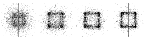
(Made with Scilab, www.scilab.org) Expected distributions for zeros of random polynomials $f_{p}$ of degree $p$ visualized using the law of large numbers. From the left to the right depicted are the zeros contained in $[-2,2]\times[-2,2]\subset\mathbb{C}$ of $5000$ random polynomials of degree 4, 1667 of degree $12$, 833 of degree 24, and 500 of degree 40. The polynomials $f_{p}$ are randomly chosen with respect to the Gaussian distribution on $(\mathbb{C}_{p}[z],(\cdot,\cdot))$. The pictures were developed during a joint project with Gerrit Herrmann (Regensburg).

Figure 1. Zero distributions for the square

To obtain the pictures we use the following strategy. Using the law of large numbers we can approximate the expected distribution by choosing a sequence of random polynomials of fixed degree $p$, that is

$$\frac{1}{2\pi Np}\,\Delta\sum_{m=1}^{N}\log|f^{(m)}_{p}|\to p^{-1}\mathbb{E}(Z_{f_{p}}),\,\,\,N\to\infty.$$

By drawing the zeros of each of these polynomials as points in the plane we just illustrate the support of the measure $\Delta\sum_{m=1}^{N}\log|f^{(m)}_{p}|$. Therefore we choose $N$ depending on $p$ such that $Np$ is constant. Moreover, the fact that we can take $N$ small (and even $N=1$) for $p$ large is consistent with the second assertion of Theorem 2.2 (see (2.12)).

Let us explain now how to construct the random polynomials $f_{p}$. For $p$ fixed we compute a positive definite hermitian $(p+1)\times(p+1)$ matrix $S=(s_{lj})_{0\leq l,j\leq p}$ with entries $s_{lj}=(z^{l},z^{j})$. Applying the Cholesky decomposition to $S$ we find (after inversion) a matrix $R=(r_{lj})_{0\leq l,j\leq p}$ with $\operatorname{Id}=R^{*}SR$. Hence, we have that $s_{0},\ldots,s_{p}$ is an orthonormal Basis where $s_{j}$ is given by

$$s_{j}(z)=\sum_{l=0}^{p}r_{lj}z^{l},\,\,0\leq j\leq p.$$

Choosing Gaussian distributed (pseudo) random numbers $a_{0},a_{1},\ldots,a_{p}$ leads to the desired random polynomial $f_{p}$.

5.2. Random $SU_{2}$-polynomials with uniformly distributed coefficients

We consider random $SU_{2}$-polynomials $f_{p}$ of degree $p$, that is

$$f_{p}(z)=\sum_{j=0}^{p}a_{j}\sqrt{(p+1)\binom{p}{j}}\,z^{j}$$

where $a_{0},\ldots,a_{p}$ are i.i.d. real random numbers uniformly distributed on the interval $[0,1]$. Setting $s_{j}(z)=\sqrt{(p+1)\binom{p}{j}}z^{j}$, $0\leq j\leq p$ we have that $s_{0},\ldots,s_{p}$ is an orthonormal basis for the space $(\mathbb{C}_{p}[z],(\cdot,\cdot)_{p})$ consisting of polynomials in one complex variable of degree at most $p$ with inner product $(\cdot,\cdot)_{p}$ given by

$$(f,g)_{p}=\int_{\mathbb{C}}\frac{f(z)\overline{g(z)}}{\pi(1+|z|^{2})^{p+2}}\,d\lambda_{2}(z),\,\,\,f,g\in\mathbb{C}_{p}[z].$$

Theorem 3.1 applies in this case with the measures $\sigma_{p+1}$ from Proposition 4.7. It implies that for $p\to\infty$ the zeros of $f_{p}$ distribute to the measure

$$d\mu(z)=\frac{1}{\pi(1+|z|^{2})^{2}}\,d\lambda_{2}(z).$$

The measure $d\mu$ is visualized in Figure 2. Proceeding as in Example I we obtain pictures for the expected distributions of zeros $p^{-1}\mathbb{E}(Z_{f_{p}})$ for various $p$ (see Figure 3). The computations in this example are easier since an orthonormal basis for $(\mathbb{C}_{p}[z],(\cdot,\cdot)_{p})$ is already given.

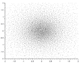
(Made with Scilab, www.scilab.org) All points, which lie in the domain $[-2,2]\times[-2,2]\subset\mathbb{C}$, out of 10240 randomly chosen points in $\mathbb{C}$ with respect to the distribution $d\mu$.

Figure 2. Visualization of $d\mu$

In Figure 3, starting with random polynomials of degree $p=1$, we see that all the zeros lie on the negative real axis. That is clear since polynomials of the form $z\mapsto a_{0}+a_{1}z$ with $a_{0},a_{1}\in\mathbb{R}_{+}$ have one zero given by $z=-\frac{a_{0}}{a_{1}}\in\mathbb{R}_{-}$. For degree $p=2$ we see that all the zeros have negative real part which immediately follows from solving the equation $a_{0}+a_{1}z+a_{2}z^{2}=0$ with $a_{0},a_{1},a_{2}>0$. We see that the zeros of $f_{p}$ avoid a region around the positive real axis which shrinks as $p$ becomes larger. Comparing Figure 3 to Figure 2 we see that the zeros of $f_{p}$ distribute to the measure $\nu$ as $p$ increases.

The pictures and all computations were made using Scilab (www.scilab.org). It is important to mention that all the numerical computations and approximations generate some errors which we do not specify here. Hence, we do not claim the visualization of the true expected distributions.

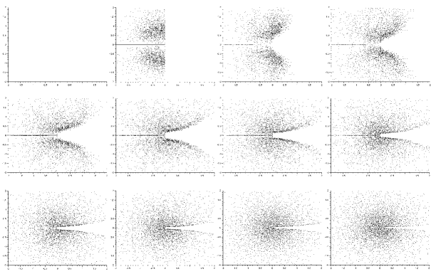
(Made with Scilab, www.scilab.org) Expected distributions for zeros of random polynomials $f_{p}$ of degree $p$ visualized using the law of large numbers. Depicted are the zeros in the domain $[-2,2]\times[-2,2]$ of $5\cdot 2^{13-j}$ random polynomials of degree $p=2^{j-1}$ with $j=1,2,\ldots,12$, starting from the upper left down to the bottom right corner. The polynomials $f_{p}$ are random $SU_{2}$-polynomials with real coefficients uniformly distributed in the interval $[0,1]$.

Figure 3. Zero distribution for $SU_{2}$-polynomials

References

- [A] A. Andreotti, Théorèmes de dépendance algébrique sur les espaces complexes pseudo-concaves, Bull. Soc. Math. France 91 (1963), 1–38.
- [Ba1] T. Bayraktar, Equidistribution of zeros of random holomorphic sections, Indiana Univ. Math. J. 65 (2016), 1759–1793.
- [Ba2] T. Bayraktar, Asymptotic normality of linear statistics of zeros of random polynomials, Proc. Amer. Math. Soc. 145 (2017), 2917–2929.
- [Ba3] T. Bayraktar, Zero distribution of random sparse polynomials, Michigan Math. J. 66 (2017), 389–419.
- [Ba4] T. Bayraktar, Expected number of real roots for random linear combinations of orthogonal polynomials associated with radial weights, Potential Anal. 48 (2018), no. 4, 59–471.
- [Ba5] T. Bayraktar, On global universality for zeros of random polynomials, Hacet. J. Math. Stat. 48 (2019), no. 2, 384–398.
- [BCM] T. Bayraktar, D. Coman and G. Marinescu, Universality results for zeros of random holomorphic sections, Trans. Amer. Math. Soc. 373 (2020), no. 6, 3765–3791.
- [B1] T. Bloom, Random polynomials and Green functions, Int. Math. Res. Not. 2005, no. 28, 1689–1708.
- [B2] T. Bloom, Weighted polynomials and weighted pluripotential theory, Trans. Amer. Math. Soc. 361 (2009), no. 4, 2163–2179.
- [BD] T. Bloom and D. Dauvergne, Universality for zeros of random polynomials, arXiv:1801.10125, 2018.
- [BL] T. Bloom and N. Levenberg, Random polynomials and pluripotential-theoretic extremal functions, Potential Anal. 42 (2015), 311–334.
- [BLPW] T. Bloom, N. Levenberg, F. Piazzon, and F. Wielonsky, Bernstein-Markov: a survey, Dolomites Research Notes on Approximation 8 (2015), 75–91.
- [BP] A. Bloch and G. Pólya, On the roots of certain algebraic equations, Proc. London Math. Soc.v 33 (1931), 102–114.
- [BS] T. Bloom and B. Shiffman, Zeros of random polynomials on , Math. Res. Lett.v 14 (2007), 469–479.
- [BT1] E. Bedford and B. A. Taylor, The Dirichlet problem for a complex Monge-Ampère equation, Invent. Math. 37 (1976), 1–44.
- [BT2] E. Bedford and B. A. Taylor, A new capacity for plurisubharmonic functions, Acta Math. 149 (1982), 1–40.
- [BBH] E. Bogomolny, O. Bohigas and P. Leboeuf, Quantum chaotic dynamics and random polynomials, J. Stat. Phys. 85 (1996), 639–679.
- [CM1] D. Coman and G. Marinescu, Equidistribution results for singular metrics on line bundles, Ann. Sci. Éc. Norm. Supér. (4) 48 (2015), 497–536.
- [CM2] D. Coman and G. Marinescu, Convergence of Fubini-Study currents for orbifold line bundles, Internat. J. Math. 24 (2013), 1350051, 27 pp.
- [CM3] D. Coman and G. Marinescu, On the approximation of positive closed currents on compact Kähler manifolds, Math. Rep. (Bucur.) 15(65) (2013), no. 4, 373–386.
- [CMM] D. Coman, X. Ma, and G. Marinescu, Equidistribution for sequences of line bundles on normal Kähler spaces, Geom. Topol. 21 (2017), no. 2, 923–962.
- [Da] M. Das, Real zeros of a random sum of orthogonal polynomials, Proc. Amer. Math. Soc. 27 (1971), 147–153.
- [De] J.-P. Demailly, Singular Hermitian metrics on positive line bundles, in Complex algebraic varieties (Bayreuth, 1990), Lecture Notes in Math. 1507, Springer, Berlin, 1992, 87–104.
- [DMM] T.-C. Dinh, X. Ma and G. Marinescu, Equidistribution and convergence speed for zeros of holomorphic sections of singular Hermitian line bundles, J. Funct. Anal. 271 (2016), no. 11, 3082–3110.
- [DMS] T.-C. Dinh and G. Marinescu and V. Schmidt, Asymptotic distribution of zeros of holomorphic sections in the non-compact setting, J. Stat. Phys. 148 (2012), no. 1, 113–136.
- [DS1] T.-C. Dinh and N. Sibony, Distribution des valeurs de transformations méromorphes et applications, Comment. Math. Helv. 81 (2006), 221–258.
- [DS2] T.-C. Dinh and N. Sibony, Super-potentials of positive closed currents, intersection theory and dynamics, Acta Math. 203 (2009), 1–82.
- [EK] A. Edelman and E. Kostlan, How many zeros of a random polynomial are real?, Bull. Amer. Math. Soc. (N.S.) 32 (1995), 1–37.
- [EO] P. Erdős and A. C. Offord, On the number of real roots of a random algebraic equation, Proc. London Math. Soc. (3) 6 (1956), 139–160.
- [ET] P. Erdős and P. Turán, On the distribution of roots of polynomials, Ann. of Math. (2) 51 (1950), 105–119.
- [GZ] V. Guedj and A. Zeriahi, Intrinsic capacities on compact Kähler manifolds, J. Geom. Anal. 15 (2005), 607–639.
- [H] J. M. Hammersley, The zeros of a random polynomial, Proceedings of the Third Berkeley Symposium on Mathematical Statistics and Probability, 1954-1955, vol. II, pp. 89–111. University of California Press, Berkeley and Los Angeles, 1956.
- [HS] R. Holowinsky, K. Soundararajan, Mass equidistribution for Hecke eigenforms, Ann. Math. (2) 172 (2010), 1517–1528.
- [IM1] I. A. Ibragimov and N. B. Maslova, The mean number of real zeros of random polynomials. I. Coefficients with zero mean, Teor. Verojatnost. i Primenen. 16 (1971), 229–248.
- [IM2] I. A. Ibragimov and N. B. Maslova, The mean number of real zeros of random polynomials. II. Coefficients with a nonzero mean, Teor. Verojatnost. i Primenen. 16 (1971), 495–503.
- [K] M. Kac, On the average number of real roots of a random algebraic equation, Bull. Amer. Math. Soc. 49 (1943), 314–320.
- [LO1] J. E. Littlewood and A. C. Offord, On the number of real roots of a random algebraic equation. III, Rec. Math. [Mat. Sbornik] N.S. 12(54) (1943), 277–286.
- [LO2] J. E. Littlewood and A. C. Offord, On the distribution of the zeros and -values of a random integral function. I, J. London Math. Soc. 20 (1945), 130–136.
- [LO3] J. E. Littlewood and A. C. Offord, On the distribution of zeros and -values of a random integral function. II, Ann. of Math. (2) 49 (1948), 885–952; erratum 50 (1949), 990–991.
- [LPX] D.S. Lubinsky, I.E. Pritsker, and X. Xie, Expected number of real zeros for random linear combinations of orthogonal polynomials, Proc. Amer. Math. Soc. 144 (2016), 1631–1642.
- [MM] X. Ma and G. Marinescu, Holomorphic Morse Inequalities and Bergman Kernels, Progress in Math., vol. 254, Birkhäuser, Basel, 2007, xiii, 422 pp.
- [NS] F. Nazarov and M. Sodin, Correlation functions for random complex zeroes: strong clustering and local universality, Comm. Math. Phys. 310 (2012), 75–98.
- [NV] S. Nonnenmacher and A. Voros, Chaotic eigenfunctions in phase space, J. Stat. Phys. 92 (1998), no. 3-4, 451–518.
- [RS] Z. Rudnick and P. Sarnak, The behavior of eigenstates of arithmetic hyperbolic manifolds, Comm. Math. Phys. 161 (1994), 195–213.
- [SaT] E. B. Saff and V. Totik, Logarithmic Potentials with External Fields, Grundlehren der Mathematischen Wissenschaften [Fundamental Principles of Mathematical Sciences] 316, Springer-Verlag, Berlin, 1997. Appendix B by Thomas Bloom.
- [Sh] B. Shiffman, Convergence of random zeros on complex manifolds, Sci. China Ser. A 51 (2008), 707–720.
- [SZ1] B. Shiffman and S. Zelditch, Distribution of zeros of random and quantum chaotic sections of positive line bundles, Comm. Math. Phys. 200 (1999), 661–683.
- [SZ2] B. Shiffman and S. Zelditch, Equilibrium distribution of zeros of random polynomials, Int. Math. Res. Not. 2003, no. 1, 25–49.
- [SZ3] B. Shiffman and S. Zelditch, Number variance of random zeros on complex manifolds, Geom. Funct. Anal. 18 (2008), 1422–1475.
- [SZ4] B. Shiffman and S. Zelditch, Number variance of random zeros on complex manifolds, II: smooth statistics, Pure Appl. Math. Q. 6 (2010), 1145–1167.
- [Si] J. Siciak, Extremal plurisubharmonic functions in , Ann. Polon. Math 39 (1981), 175–211.
- [SoT] M. Sodin and B. Tsirelson, Random complex zeroes. I. Asymptotic normality, Israel J. Math. 144 (2004), 125–149.
- [TV] T. Tao and V. Vu, Local universality of zeroes of random polynomials, Int. Math. Res. Not. 2015, no. 13, 5053–5139.
- [V] R. J. Vanderbei, The complex roots of random sums, arXiv:1508.05162, 2015.