A density result on Orlicz-Sobolev spaces in the plane

Abstract.

We show the density of smooth Sobolev functions $W^{k,\infty}(\Omega)\cap C^{\infty}(\Omega)$ in the Orlicz-Sobolev spaces $L^{k,\Psi}(\Omega)$ for bounded simply connected planar domains $\Omega$ and doubling Young functions $\Psi$.

1. Introduction

Orlicz-Sobolev spaces appear naturally in analysis as generalizations of the usual Sobolev spaces, for instance when one studies sharp assumptions for mappings of finite distortion [16, 18]. Orlicz-Sobolev spaces appear also in many other contexts and have been studied by their own right, see for instance [1, 2, 5, 6, 7, 9, 8, 12, 11, 14, 13, 15, 24, 30, 33] for a sample of the literature.

An important basic question in the theory of function spaces is the relation between different spaces. Answers to this question can be given for instance in terms of embeddings and density results. In this paper, we show that in Orlicz-Sobolev spaces on bounded simply connected planar domains we can approximate functions with bounded derivatives if we consider only the highest order derivatives in the norm.

Theorem 1.1.

Let $k\in\mathbb{N}$, $\Psi$ be a doubling Young function, and $\Omega\subset\mathbb{R}^{2}$ be a bounded simply connected domain. Then the subspace $W^{k,\infty}(\Omega)\cap C^{\infty}(\Omega)$ is dense in the space $L^{k,\Psi}(\Omega).$

Recall that for a domain $\Omega\subset\mathbb{R}^{2}$ and a Young function $\Psi$, the version of the Orlicz-Sobolev space $L^{k,\Psi}(\Omega)$ used in Theorem 1.1 is defined as

$$L^{k,\Psi}(\Omega)=\left\{f\in L^{\Psi}(\Omega):\nabla^{\alpha}f\in L^{\Psi}(\Omega)\;\text{ if }|\alpha|=k\right\}.$$

The space $L^{k,\Psi}(\Omega)$ is equipped with the semi-norm $\sum_{|\alpha|=k}\left\|\nabla^{\alpha}f\right\|_{L^{\Psi}(\Omega)}$, where
$\|\cdot\|_{L^{\Psi}(\Omega)}$ is the Luxemburg norm. See Section 2 for more basic information on Orlicz and Orlicz-Sobolev spaces.

We will use a Whitney decomposition of the domain $\Omega\subset\mathbb{R}^{2}$ and make a polynomial approximation near the boundary $\partial\Omega$. The validity of the approximation is proven using a $\Psi-\Psi$ Poincaré inequality. The form of the polynomial approximation we use here was introduced in [28], where a density result was shown for homogeneous Sobolev spaces on simply connected planar domains. This was then extended to Gromov hyperbolic domains in higher dimensions in [27]. In turn, both of these results were generalizations of density results for first order Sobolev spaces [23, 22] which were partly motivated by the recent progress on planar Sobolev extension domains [21, 31].

Although for every domain smooth functions are dense in $W^{k,p}(\Omega)$ [26] and, more generally, in $W^{k,\Psi}(\Omega)$ for doubling $\Psi$ [10], the derivatives of the approximating smooth functions might blow up near the boundary. Therefore, the density of other function spaces, such as $W^{k,q}(\Omega)$ in $W^{k,p}(\Omega)$ might be false, see [20, 22] for this, and for instance [3, 19, 29] for earlier counter examples on other function spaces. The density of global smooth functions in $W^{1,p}(\Omega)$ is known for instance for Jordan domains [25, 23], but the case for higher order Sobolev spaces is still open. Similarly, in the case $k\geq 2$, the density result presented in Theorem 1.1 remains still open for the full Orlicz-Sobolev space $W^{k,\Psi}(\Omega)$ as well as for the usual Sobolev space $W^{k,p}(\Omega)$.

In the same way as for the first order Sobolev spaces [23], for $W^{1,\Psi}(\Omega)$ we get a better density result as a corollary of Theorem 1.1. This is simply because we may first cut a function in $W^{1,\Psi}(\Omega)$ from above and below introducing a small error in the norm, so that the function becomes an $L^{\infty}(\Omega)$ function. The remaining approximations do not change the fact that the function is in $L^{\infty}(\Omega)$.

Corollary 1.2.

Let $\Psi$ be a doubling Young function and $\Omega\subset\mathbb{R}^{2}$ be a bounded simply connected domain. Then the subspace $W^{1,\infty}(\Omega)\cap C^{\infty}(\Omega)$ is dense in the space $W^{1,\Psi}(\Omega).$

The paper is organized as follows. In Section 2 we recall the Whitney decomposition and list the required prerequisites from the Orlicz theory. In Section 3 we give a partition of unity for the domain using a Whitney type decomposition. Finally, in Section 4 we show the proof of Theorem 1.1.

2. Preliminaries

In this paper, we will usually denote constants by $C$. The value of the constant might change between appearances, even in a chain of inequalities, but the dependence of the constant on a set of fixed parameters is always stated. Sometimes, to clarify the dependence, the parameters are written inside parentheses $C(\cdot)$.

2.1. Whitney decomposition

In this section we recall the Whitney decomposition of a domain in $\mathbb{R}^{d}$. Such decomposition is standard in analysis, see for instance Whitney [34] or the book of Stein [32, Chapter VI]. We will use a version of the decomposition that was used in [28].

We denote the sidelength of a square $Q$ by $\ell(Q)$. For notational convenience we start the Whitney decomposition below from squares with sidelength $2^{-1}$. Formally, since we are working with doubling Young functions, by rescaling, we may consider all bounded domains $\Omega\subset\mathbb{R}^{2}$ to have $\mathrm{diam}(\Omega)\leq 1$ in which case no Whitney decomposition would have squares larger than the ones used below regardless of the starting scale. A Whitney decomposition in the plane consists of dyadic squares. Let us first recall those.

Definition 2.1 (Dyadic squares).

A dyadic interval in $\mathbb{R}$ is an interval of the form
$[m2^{-k},(m+1)2^{-k}]$ where $m,k\in\mathbb{Z}.$ A dyadic square in $\mathbb{R}^{2}$ is a product of dyadic intervals of the same length. That is, a dyadic square is a set of the form

$$[m_{1}2^{-k},(m_{1}+1)2^{-k}]\times[m_{2}2^{-k},(m_{2}+1)2^{-k}]$$

for some integers $m_{1}$ and $,m_{2}$.

Let us now define a Whitney decomposition following Lemma 2.3 in [28].

Definition 2.2 (Whitney decomposition).

Let $\Omega$ be a bounded open subset of $\mathbb{R}^{2}$. A Whitney decomposition is a collection $\tilde{\mathcal{F}}$ of dyadic squares inside $\Omega$ satisfying the following properties.

1. $\Omega=\bigcup_{Q\in\tilde{\mathcal{F}}}Q$

2. $\ell(Q)<\mathrm{dist}(Q,\Omega^{c})\leq 3\sqrt{2}\ell(Q)=3\mathrm{diam}(Q)$ for all $Q\in\tilde{\mathcal{F}}$

3. $\mathrm{int\,}Q_{1}\cap\mathrm{int\,}Q_{2}=\emptyset$ for all $Q_{1},Q_{2}\in\tilde{\mathcal{F}},Q_{1}\neq Q_{2}$

4. If $Q_{1},Q_{2}\in\tilde{\mathcal{F}}$ and $Q_{1}\cap Q_{2}\neq\emptyset$, then $\frac{\ell(Q_{1})}{\ell(Q_{2})}\leq 2$.

Suppose $Q_{1},\dots,Q_{m}$ are Whitney squares such that $Q_{j}$ and $Q_{j+1}$ touch and $\frac{1}{4}\leq\frac{\ell(Q_{j})}{\ell(Q_{j+1})}\leq 4$ for all $j,1\leq j\leq m-1.$ We say then $\{Q_{1},\dots,Q_{m}\}$ is a chain connecting $Q_{1}$ to $Q_{m}$ and define the length of that chain to be the integer $m$.

2.2. Orlicz Spaces

Definition 2.3.

A function $\Psi\colon[0,\infty)\rightarrow[0,\infty]$ is a Young function if

$$\Psi(s)=\displaystyle\int_{0}^{s}\psi(t)\,{\mathrm{d}}t,$$ (2.1)

where $\psi:[0,\infty]\rightarrow[0,\infty]$ is an increasing, left continuous function which is neither identically zero nor identically infinite on $(0,\infty)$ and which satisfies $\psi(0)=0.$

A Young function $\Psi$ is convex, increasing, left continuous, $\Psi(0)=0$ and $\Psi(t)\rightarrow\infty$ as $t\rightarrow\infty.$ A continuous Young function with the properties $\Psi(t)=0,$ only if $t=0,$ $\Psi(t)/t\rightarrow\infty$ as $t\rightarrow\infty$ and $\Psi(t)/t\rightarrow 0$ as $t\rightarrow 0$ is called an $N$-function.

It follows easily from the convexity and $\Psi(0)=0$, that the function $t\rightarrow\Psi(t)/t$ is increasing. This implies that if $\Psi$ is strictly increasing, then the function $\Psi^{-1}(t)/t$ is decreasing. A Young function $\Psi$ is doubling if there is a constant $C>0$ such that

$$\Psi(2t)\leq C\Psi(t)$$ (2.2)

for each $t\geq 0$. The smallest constant $C$ satisfying (2.2) is called the doubling constant of $\Psi$.

Definition 2.4.

Given a doubling Young function $\Psi$ and an open set $\Omega\subset\mathbb{R}^{2}$, we denote by $L^{\Psi}(\Omega)$, the Orlicz space associated to $\Psi$, defined by

$$L^{\Psi}(\Omega)=\left\{u\colon\Omega\rightarrow\mathbb{R}:\displaystyle\int_{\Omega}\Psi(|u(x)|)\,{\mathrm{d}}x<\infty\right\}.$$

$L^{\Psi}(\Omega)$ is a Banach space, when equipped with the Luxemburg norm

$$\|u\|_{L^{\Psi}(\Omega)}=\inf\left\{k>0\,:\,\displaystyle\int_{\Omega}\Psi(k^{-1}|u(x)|)\,{\mathrm{d}}x\leq 1\right\}.$$

We will not use the Luxemburg norm in this paper, but work with the integrals. This is justified by the following fact.

Lemma 2.5.

Let $\Psi$ be a doubling Young function. Then

$$\|u_{i}-u\|_{L^{\Psi}(\Omega)}\to 0\qquad\text{as }i\to\infty$$

if and only if

$$\int_{\Omega}\Psi(|u_{i}(x)-u(x)|)\,{\mathrm{d}}x\to 0\qquad\text{as }i\to\infty.$$

A direct consequence of Jensen’s inequality is the following.

Lemma 2.6.

Let $\Psi$ be a Young function, $u\in L_{\text{loc}}^{1}(\mathbb{R}^{2})$ and $A\subset\mathbb{R}^{2}$ of positive and finite measure, then

$$\Psi\left(\fint_{A}|u(x)|\,{\mathrm{d}}x\right)\leq\fint_{A}\Psi(|u(x)|)\,{\mathrm{d}}x,$$

where $u_{A}=\fint_{A}|u(x)|\,{\mathrm{d}}x$ is the average integral.

2.3. Poincaré inequalities and polynomial approximation

From now on, $\Psi$ always refers to a doubling Young function. We will construct an approximation by replacing the original function by approximating polynomials near the boundary of the domain. For this purpose, we will need a few lemmas regarding the polynomials. Here and later on by $|E|$ we denote the Lebesgue measure of a set $E\subset\mathbb{R}^{2}$.

Lemma 2.7.

Let $Q$ be any square in $\mathbb{R}^{2}$ and $P$ be a polynomial of degree $k$ defined in $\mathbb{R}^{2}$. Let $E,F\subset Q$ be such that $|E|,|F|>\eta|Q|$ where $\eta>0$. Then

$$\int_{E}\Psi(|P(x)|)\,{\mathrm{d}}x\leq C\int_{F}\Psi(|P(x)|)\,{\mathrm{d}}x,$$

where the constant $C$ depends only on $\eta$, $k$ and the doubling constant of $\Psi$.

Proof.

Since any two norms on a finite dimensional vector space are comparable, there exists a constant $\delta>0$ depending only on $k$ and $\eta$ so that the set

$$\tilde{F}:=\left\{x\in F:|P(x)|\geq\delta\max_{y\in Q}|P(y)|\right\}$$

satisfies $|\tilde{F}|\geq\frac{1}{2}|F|$.

Therefore, by applying monotonicity and doubling properties on $\Psi$ we obtain

$$\displaystyle\int_{F}\Psi(|P(x)|)\,{\mathrm{d}}x \geq\displaystyle\int_{\tilde{F}}\Psi(|P(x)|)\,{\mathrm{d}}x\geq\displaystyle\int_{\tilde{F}}\Psi(\delta\max_{y\in Q}|P(y)|)\,{\mathrm{d}}x$$

$$\geq C\displaystyle\int_{\tilde{F}}\Psi(\max_{y\in Q}|P(y)|)\,{\mathrm{d}}x=C|\tilde{F}|\Psi(\max_{y\in Q}|P(y)|)$$

$$\geq\frac{C|\tilde{F}|}{|Q|}\displaystyle\int_{Q}\Psi(|P(x)|)\,{\mathrm{d}}x\geq C\displaystyle\int_{Q}\Psi(|P(x)|)\,{\mathrm{d}}x$$

$$\geq C\displaystyle\int_{E}\Psi(P(x))\,{\mathrm{d}}x,$$

which gives the claim. ∎

Given a function $u\in C^{\infty}(\Omega)$, degree $k\in\mathbb{N}$, and a bounded set $E\subset\Omega$ with $|E|>0$, we define (see [17]) the polynomial approximation of $u$ in $E$, $P_{k}(u,E)$ to be the polynomial of order $k-1$ which satisfies

$$\int_{E}\nabla^{\alpha}(u-P_{k}(u,E))=0$$

for each $\alpha=(\alpha_{1},\alpha_{2})$ such that $|\alpha|=\alpha_{1}+\alpha_{2}\leq k-1$. Once $k$ is fixed, we denote the polynomial approximation of $u$ in a dyadic square $Q$ as $P_{Q}$.

Proposition 2.8 ($\Psi-\Psi$ Poincaré inequality).

Let $k,m\in\mathbb{N}$. There exists a constant $C$ depending only on $k$, $m$ and the doubling constant of $\Psi$ such that for any domain $\Omega\subset\mathbb{R}^{2}$, a chain $\{Q_{i}\}_{i=1}^{m}$ of dyadic squares in $\Omega$, and a function $u\in L^{k,\Psi}(\Omega)$ we have

$$\fint_{E}\Psi\left(\frac{|u(x)-P_{E}(x)|}{\ell(Q_{1})^{k}}\right)\,{\mathrm{d}}x\leq C\fint_{E}\Psi(|\nabla^{k}u(x)|)\,{\mathrm{d}}x,$$

where we have abbreviated $E=\bigcup_{i=1}^{m}Q_{i}$.

Proof.

By [4, Lemma 1] the claim is true for $k=1$ in the case where $E$ is convex. By a change of variables, the claim extends to the case $k=1$ and $E=\bigcup_{i=1}^{m}Q_{i}$, for the chain $\{Q_{i}\}_{i=1}^{m}$. What remains to show is the case $k>1$.

We do this by induction. Suppose the claim is true for the order $k-1$. Then, using the Poincaré inequality first for the $k-1$ orders and the for the first order, we obtain

$$\fint_{E}\Psi\left(\frac{|u(x)-P_{E}(x)|}{\ell(Q_{1})^{k}}\right)\,{\mathrm{d}}x \leq C\fint_{E}\Psi\left(\frac{|\nabla^{k-1}(u(x)-P_{E}(x))|}{\ell(Q_{1})}\right)\,{\mathrm{d}}x$$

$$\leq C\fint_{E}\Psi\left(|\nabla^{k}(u(x)-P_{E}(x))|\right)\,{\mathrm{d}}x$$

$$=C\fint_{E}\Psi\left(|\nabla^{k}u(x)|\right)\,{\mathrm{d}}x.\qed$$

Lemma 2.9.

Let $\Omega\subset\mathbb{R}^{2}$ be a bounded simply connected domain and $\tilde{\mathcal{F}}$ a Whitney decomposition of $\Omega.$ Let $\{Q_{i}\}_{i=1}^{m}$ be a chain of dyadic squares in $\tilde{\mathcal{F}}$. Then there exists a constant $C$ depending only on $k$, $m$ and the doubling constant of $\Psi$ such that if $|\alpha|\leq k,$ we have

$$\int_{Q_{1}}\Psi\left(\frac{\nabla^{\alpha}P_{Q_{1}}-\nabla^{\alpha}P_{Q_{m}}}{\ell(Q_{1})^{k-|\alpha|}}\right)\leq C\int_{\bigcup_{i=1}^{m}Q_{i}}\Psi(|\nabla^{k}u|).$$

Proof.

Let us abbreviate $E=\bigcup_{i=1}^{m}Q_{i}$. Now, using the triangle inequality, Lemma 2.7, the doubling property of $\Psi$, then triangle inequality again and Lemma 2.8 we obtain

$$\begin{split}\displaystyle\int_{Q_{1}}\Psi&\left(\displaystyle\dfrac{|\nabla^{\alpha}P_{Q_{1}}-\nabla^{\alpha}P_{Q_{m}}|}{\ell(Q_{1})^{k-|\alpha|}}\right)\\ &\leq\displaystyle\int_{Q_{1}}\Psi\left(\displaystyle\dfrac{|\nabla^{\alpha}P_{Q_{1}}-\nabla^{\alpha}P_{Q_{m}}+\nabla^{\alpha}P_{E}-\nabla^{\alpha}P_{E}|}{\ell(Q_{1})^{k-|\alpha|}}\right)\\ &\leq C\displaystyle\int_{Q_{1}}\Psi\left(\displaystyle\dfrac{|\nabla^{\alpha}P_{Q_{1}}-\nabla^{\alpha}P_{E}|}{\ell(Q_{1})^{k-|\alpha|}}\right)+C\displaystyle\int_{Q_{m}}\Psi\left(\displaystyle\dfrac{\nabla^{\alpha}P_{Q_{m}}-\nabla^{\alpha}P_{E}|}{\ell(Q_{m})^{k-|\alpha|}}\right)\\ &\leq C\displaystyle\int_{Q_{1}}\Psi\left(\frac{|\nabla^{\alpha}(u-P_{Q_{1}})|}{\ell(Q_{1})^{k-|\alpha|}}\right)+C\displaystyle\int_{Q_{m}}\Psi\left(\frac{|\nabla^{\alpha}(u-P_{Q_{m}})|}{\ell(Q_{m})^{k-|\alpha|}}\right)\\ &\quad+C\displaystyle\int_{E}\Psi\left(\frac{|\nabla^{\alpha}(u-P_{E})|}{\ell(Q_{1})^{k-|\alpha|}}\right)\\ &\leq C\displaystyle\int_{\bigcup_{i=1}^{m}Q_{i}}\Psi(|\nabla^{k}u|).\qed\end{split}$$

3. Decomposition and partition of unity

In this section we recall the decomposition of the domain $\Omega$ and the associated partition of unity that was obtained in [28]. In order to make the comparison between this paper and [28] easy, we use here the notation from [28].

3.1. Decomposition of the domain

We fix a square $Q_{0}$, which is one of the largest Whitney squares in $\Omega$. For each $n\in\mathbb{N}$, the domain $\Omega$ is then divided into a core part $D_{n}$, and a boundary layer, which is the union of sets $\tilde{H}_{i}$, see Figure 1.

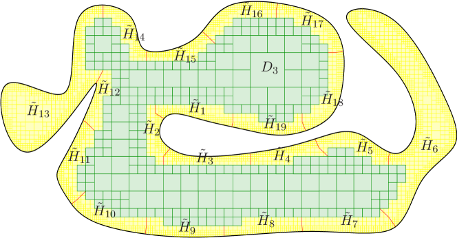
Figure 1. The domain $\Omega$ is decomposed into a core part $D_{3}$ (obtained as a connected component of a union of Whitney squares) and boundary parts $\tilde{H}_{i}$. A partition of unity is made using this decomposition.

The core part $D_{n}$ is the connected component containing $Q_{0}$ of the interior of the union of Whitney squares of side-length at least $2^{-n}$. The construction of the boundary parts $\{\tilde{H}_{i}\}_{i=1}^{l}$ is more involved. The sets $\tilde{H}_{i}$ are labeled so that $\tilde{H}_{i}\cap\tilde{H}_{j}\neq\emptyset$ if and only if $|i-j|\leq 1$ in a cyclical manner.

The sets $\tilde{H}_{i}$ are expanded by taking a connected component $H_{i}$ of a $2^{-n-3}$ neighbourhood of $\tilde{H}_{i}$. The main property of the decomposition is that these expanded sets still satisfy $H_{i}\cap H_{j}\neq\emptyset$ if and only if $|i-j|\leq 1$ in a cyclical manner (Lemma 3.4 in [28]). Moreover, since the neighbourhoods are taken in the Euclidean distance, we may use an Euclidean partition of unity.

For each $i$ we associate a Whitney square $Q_{i}\subset D_{n}$ of side length $2^{-n}$ so that $H_{i}\cap Q_{i}\neq\emptyset$ and, more importantly, if $|i-j|\leq 1$, there is a chain of Whitney squares $\mathcal{Q}_{i,j}$ with length bounded by a universal constant connecting $Q_{i}$ and $Q_{j}$.

3.2. Partition of unity

Using the decomposition of the domain $\Omega$ introduced above, we make a partition of unity for the domain. The partition of unity consists of functions $\psi_{i}$, $i\in\{0,\dots,l\}$ with the following properties:

1. The function $\psi_{0}$ is supported in $B(D_{n},\frac{2^{-n}}{10})$.

2. For $i\geq 1$ the function $\psi_{i}$ is supported in $H_{i}$.

3. For all $i$, $0\leq\psi_{i}\leq 1$.

4. $\sum\psi_{i}\equiv 1$ on $\Omega$.

5. For all $i$, $|\nabla^{\alpha}\psi_{i}|\leq C({\alpha})2^{-n|\alpha|}$ for all multi-indeces $\alpha$.

4. Proof of Theorem 1.1

In this section we prove Theorem 1.1, using the results of Section 2 and the partition of union from [28] that was recalled in Section 3. The polynomial approximation is exactly the same as in [28]. What is different is the way the estimates are carried out using Poincaré inequalities. Since the usual Poincaré inequality is replaced by a $\Psi-\Psi$ Poincaré inequality (Proposition 2.8), we need to be more careful with the chains of inequalities.

Given a function $u\in L^{k,\Psi}(\Omega)$ and $\varepsilon>0$, our aim is to find a function $u_{\varepsilon}\in W^{k,\infty}(\Omega)\cap C^{\infty}(\Omega)$ satisfying $\left\|\nabla^{k}u_{\varepsilon}-\nabla^{k}u\right\|_{L^{\Psi}(\Omega)}\lesssim\varepsilon.$ We start by noting that we may assume $u\in L^{k,\Psi}(\Omega)\cap C^{\infty}(\Omega)$, since smooth functions are dense in $L^{k,\Psi}(\Omega)$, see [10].

For $n\in\mathbb{N}$ fixed, we let $D_{n}$ and $\{H_{i}\}_{i=1}^{l}$ be as in Section 3. With these we define a function $u_{n}\in W^{k,\infty}(\Omega)\cap C^{\infty}(\Omega)$ by setting for all $x\in\Omega$

$$u_{n}(x)=\varphi_{0}(x)u(x)+\sum_{i=1}^{l}\varphi_{i}(x)P_{i}(x),$$

where we have abbreviated $P_{i}:=P_{Q_{i}}$ with the choice of squares $Q_{i}$ done in Section 3.2. Clearly, $u_{n}\in W^{k,\infty}(\Omega)\cap C^{\infty}(\Omega)$. Therefore, what remains to show is that

$$\left\|\nabla^{k}u_{n}-\nabla^{k}u\right\|_{L^{\Psi}(\Omega)}\to 0,\qquad\text{as }n\to\infty.$$ (4.1)

First of all, by the definition of $u_{n}$, we have

$$u_{n}(x)=u(x)\qquad\text{ for all }x\in\{z\in\Omega\,:\,\varphi_{0}(z)=1\}\subset D_{n-1}.$$

Also, for all $i\in\{1\dots,l\}$, since $P_{i}$ is a degree $n-1$ polynomial, we have

$$\nabla^{k}u_{n}(x)=0\qquad\text{ for all }x\in\{z\in\Omega\,:\,\varphi_{i}(z)=1\}.$$

Therefore,

$$\left\|\nabla^{k}u_{n}-\nabla^{k}u\right\|_{L^{\Psi}(\Omega)} =\left\|\nabla^{k}u_{n}-\nabla^{k}u\right\|_{L^{\Psi}(\{\varphi_{0}\neq 1\})}$$

$$\leq\left\|\nabla^{k}u\right\|_{L^{\Psi}(\Omega\setminus D_{n-1})}+\left\|\nabla^{k}u_{n}\right\|_{L^{\Psi}(\bigcup_{i=1}^{l}A_{i})},$$

where we have written $A_{i}:=\{x\in\Omega\,:\,0<\varphi_{i}(x)<1\}$ for $i\in\{1,\dots,l\}$. Since the sets $D_{n}$ increasingly exhaust the domain $\Omega$, we have

$$\left\|\nabla^{k}u\right\|_{L^{\Psi}(\Omega\setminus D_{n-1})}\to 0\qquad\text{as }n\to\infty.$$

Thus, it remains to show that

$$\left\|\nabla^{k}u_{n}\right\|_{L^{\Psi}(\bigcup_{i=1}^{l}A_{i})}\to 0\qquad\text{as }n\to\infty,$$ (4.2)

or equivalently, via Lemma 2.5, that for each multi-index $\alpha$ with $|\alpha|=k$ we have

$$\int_{\bigcup_{i=1}^{l}A_{i}}\Psi(|\nabla^{\alpha}u_{n}(x)|)\to 0\qquad\text{as }n\to\infty.$$ (4.3)

In order to show (4.3), we estimate for each $i\in\{1,\dots,l\}$ and multi-index $\alpha$ with $|\alpha|=k$, by using the triangle inequality and Jensen’s inequality

$$\displaystyle\int_{A_{i}}\Psi(|\nabla^{\alpha}u_{n}(x)|)\,{\mathrm{d}}x =\displaystyle\int_{A_{i}}\Psi\left(\left|\nabla^{\alpha}\left(\varphi_{0}(x)u(x)+\sum_{j=1}^{l}\varphi_{j}(x)P_{j}(x)\right)\right|\right)\,{\mathrm{d}}x$$

$$\leq\sum_{\beta\leq\alpha}\displaystyle\int_{A_{i}}\Psi(|\nabla^{\beta}u(x)-\nabla^{\beta}P_{i}(x)||\nabla^{\alpha-\beta}\varphi_{0}(x)|)\,{\mathrm{d}}x$$

$$\quad+\sum_{\beta\leq\alpha}\displaystyle\int_{A_{i}}\sum_{j=1}^{l}\Psi(|\nabla^{\beta}P_{j}(x)-\nabla^{\beta}P_{i}(x)||\nabla^{\alpha-\beta}\varphi_{j}(x)|)\,{\mathrm{d}}x.$$

We estimate the above two terms separately.

Let us take $\beta\leq\alpha$ and write

$$\displaystyle\int_{A_{i}} \Psi(|\nabla^{\beta}u(x)-\nabla^{\beta}P_{i}(x)||\nabla^{\alpha-\beta}\varphi_{0}(x)|)\,{\mathrm{d}}x$$

$$=\sum_{Q}\displaystyle\int_{Q}\Psi(|\nabla^{\beta}u(x)-\nabla^{\beta}P_{i}(x)|C2^{n(|\alpha|-|\beta|)})\,{\mathrm{d}}x,$$

where the integral is first split into squares $Q$ for which $Q\cap A_{i}\cap A_{0}\neq\emptyset$. There are only a uniformly bounded amount of such squares $Q$, and for each such $Q$ we have

$$\displaystyle\int_{Q} \Psi(|\nabla^{\beta}u(x)-\nabla^{\beta}P_{i}(x)|C2^{n(|\alpha|-|\beta|)})\,{\mathrm{d}}x$$

$$\leq C\displaystyle\int_{Q}\Psi\left(\frac{|\nabla^{\beta}u(x)-\nabla^{\beta}P_{Q}(x)|}{2^{-n(|\alpha|-|\beta|)}}\right)\,{\mathrm{d}}x+C\displaystyle\int_{Q}\Psi\left(\frac{|\nabla^{\beta}P_{Q}(x)-\nabla^{\beta}P_{i}(x)|}{2^{-n(|\alpha|-|\beta|)}}\right)\,{\mathrm{d}}x$$

$$\leq C\displaystyle\int_{Q}\Psi(|\nabla^{k}u(x)|)\,{\mathrm{d}}x+C\displaystyle\int_{A_{i}}\Psi(|\nabla^{k}u(x)|)\,{\mathrm{d}}x,$$

using the doubling property of $\Psi$, triangle inequality, Proposition 2.8 and Lemma 2.9.

Next we estimate for $\beta\leq\alpha$,

$$\displaystyle\int_{A_{i}}\sum_{j=1}^{l} \Psi(|\nabla^{\beta}P_{j}(x)-\nabla^{\beta}P_{i}(x)||\nabla^{\alpha-\beta}\varphi_{j}(x)|)\,{\mathrm{d}}x$$

$$=\sum_{j=i-1}^{i+1}\displaystyle\int_{A_{i}}\Psi(|\nabla^{\beta}P_{j}(x)-\nabla^{\beta}P_{i}(x)|C2^{n(|\alpha|-|\beta|)})\,{\mathrm{d}}x$$

$$\leq C\sum_{j=i-1}^{i+1}\displaystyle\int_{Q_{i}}\Psi\left(\frac{|\nabla^{\beta}P_{j}(x)-\nabla^{\beta}P_{i}(x)|}{2^{-n(|\alpha|-|\beta|)}}\right)\,{\mathrm{d}}x$$

$$\leq C\sum_{j=i-1}^{i+1}\displaystyle\int_{A_{i}\cup A_{j}}\Psi(|\nabla^{k}u(x)|)\,{\mathrm{d}}x$$

using the fact that $H_{i}\cap H_{j}\neq\emptyset$ if and only if $|i-j|\leq 1$, Lemma 2.7 and Lemma 2.9.

Combining the above estimates and using the fact that there is only a uniform number of overlaps for the estimates we have

$$\int_{\bigcup_{i=1}^{l}A_{i}}\Psi(|\nabla^{\alpha}u_{n}(x)|)\leq C\displaystyle\int_{\bigcup_{i=1}^{l}A_{i}}\Psi(|\nabla^{\alpha}u(x)|),$$

giving (4.3). This proves the theorem.

References

- [1] David R. Adams and Ritva Hurri-Syrjänen, Vanishing exponential integrability for functions whose gradients belong to , J. Funct. Anal. 197 (2003), no. 1, 162–178. MR 1957679
- [2] Robert A. Adams, Sobolev spaces, Academic Press [A subsidiary of Harcourt Brace Jovanovich, Publishers], New York-London, 1975, Pure and Applied Mathematics, Vol. 65. MR 0450957
- [3] Charles J. Amick, Approximation by smooth functions in Sobolev spaces, Bull. London Math. Soc. 11 (1979), no. 1, 37–40. MR 535794
- [4] Tilak Bhattacharya and Francesco Leonetti, A new Poincaré inequality and its application to the regularity of minimizers of integral functionals with nonstandard growth, Nonlinear Anal. 17 (1991), no. 9, 833–839. MR 1131493
- [5] Jana Björn, Orlicz-Poincaré inequalities, maximal functions and -conditions, Proc. Roy. Soc. Edinburgh Sect. A 140 (2010), no. 1, 31–48. MR 2592711
- [6] Andrea Cianchi, Continuity properties of functions from Orlicz-Sobolev spaces and embedding theorems, Ann. Scuola Norm. Sup. Pisa Cl. Sci. (4) 23 (1996), no. 3, 575–608. MR 1440034
- [7] by same author, A sharp embedding theorem for Orlicz-Sobolev spaces, Indiana Univ. Math. J. 45 (1996), no. 1, 39–65. MR 1406683
- [8] Almir Joaquim de Souza, An extension operator for Orlicz-Sobolev spaces, An. Acad. Brasil. Ciênc. 53 (1981), no. 1, 9–12. MR 623636
- [9] Noel R. DeJarnette, Self improving Orlicz-Poincare inequalities, ProQuest LLC, Ann Arbor, MI, 2013, Thesis (Ph.D.)–University of Illinois at Urbana-Champaign. MR 3251391
- [10] Thomas K. Donaldson and Neil S. Trudinger, Orlicz-Sobolev spaces and imbedding theorems, J. Functional Analysis 8 (1971), 52–75. MR 0301500
- [11] David E. Edmunds, Petr Gurka, and Bohumí r Opic, Double exponential integrability of convolution operators in generalized Lorentz-Zygmund spaces, Indiana Univ. Math. J. 44 (1995), no. 1, 19–43. MR 1336431
- [12] Nicola Fusco, Pierre-Louis Lions, and Carlo Sbordone, Sobolev imbedding theorems in borderline cases, Proc. Amer. Math. Soc. 124 (1996), no. 2, 561–565. MR 1301025
- [13] Toni Heikkinen, Sharp self-improving properties of generalized Orlicz-Poincaré inequalities in connected metric measure spaces, Indiana Univ. Math. J. 59 (2010), no. 3, 957–986. MR 2779068
- [14] by same author, Characterizations of Orlicz-Sobolev spaces by means of generalized Orlicz-Poincaré inequalities, J. Funct. Spaces Appl. (2012), Art. ID 426067, 15. MR 2881765
- [15] Toni Heikkinen and Heli Tuominen, Orlicz-Sobolev extensions and measure density condition, J. Math. Anal. Appl. 368 (2010), no. 2, 508–524. MR 2643819
- [16] Tadeusz Iwaniec, Pekka Koskela, and Jani Onninen, Mappings of finite distortion: monotonicity and continuity, Invent. Math. 144 (2001), no. 3, 507–531. MR 1833892
- [17] Peter W. Jones, Quasiconformal mappings and extendability of functions in Sobolev spaces, Acta Math. 147 (1981), no. 1-2, 71–88. MR 631089
- [18] Janne Kauhanen, Pekka Koskela, Jan Malý, Jani Onninen, and Xiao Zhong, Mappings of finite distortion: sharp Orlicz-conditions, Rev. Mat. Iberoamericana 19 (2003), no. 3, 857–872. MR 2053566
- [19] Torbjörn Kolsrud, Approximation by smooth functions in Sobolev spaces, a counterexample, Bull. London Math. Soc. 13 (1981), no. 2, 167–169. MR 608104
- [20] Pekka Koskela, Removable sets for Sobolev spaces, Ark. Mat. 37 (1999), no. 2, 291–304. MR 1714767
- [21] Pekka Koskela, Tapio Rajala, and Yi Ru-Ya Zhang, A geometric characterization of planar Sobolev extension domains, Preprint.
- [22] by same author, A density problem for Sobolev spaces on Gromov hyperbolic domains, Nonlinear Anal. 154 (2017), 189–209. MR 3614650
- [23] Pekka Koskela and Yi Ru-Ya Zhang, A density problem for Sobolev spaces on planar domains, Arch. Ration. Mech. Anal. 222 (2016), no. 1, 1–14. MR 3519964
- [24] Alois Kufner, Oldˇrich John, and Svatopluk Fuˇcík, Function spaces, Noordhoff International Publishing, Leyden; Academia, Prague, 1977, Monographs and Textbooks on Mechanics of Solids and Fluids; Mechanics: Analysis. MR 0482102
- [25] John L. Lewis, Approximation of Sobolev functions in Jordan domains, Ark. Mat. 25 (1987), no. 2, 255–264. MR 923410
- [26] Norman G. Meyers and James Serrin, , Proc. Nat. Acad. Sci. U.S.A. 51 (1964), 1055–1056. MR 0164252
- [27] Debanjan Nandi, A density result for homogeneous sobolev spaces, preprint (2018).
- [28] Debanjan Nandi, Tapio Rajala, and Timo Schultz, A density result for homogeneous Sobolev spaces on planar domains, Potential Anal. (to appear).
- [29] Anthony G. O’Farrell, An example on Sobolev space approximation, Bull. London Math. Soc. 29 (1997), no. 4, 470–474. MR 1446566
- [30] M. M. Rao and Z. D. Ren, Theory of Orlicz spaces, Monographs and Textbooks in Pure and Applied Mathematics, vol. 146, Marcel Dekker, Inc., New York, 1991. MR 1113700
- [31] Pavel Shvartsman, On Sobolev extension domains in , J. Funct. Anal. 258 (2010), no. 7, 2205–2245. MR 2584745
- [32] Elias M. Stein, Singular integrals and differentiability properties of functions, Princeton Mathematical Series, No. 30, Princeton University Press, Princeton, N.J., 1970. MR 0290095
- [33] Heli Tuominen, Characterization of Orlicz-Sobolev space, Ark. Mat. 45 (2007), no. 1, 123–139. MR 2312957
- [34] Hassler Whitney, Analytic extensions of differentiable functions defined in closed sets, Trans. Amer. Math. Soc. 36 (1934), no. 1, 63–89. MR 1501735