Smart Grid Monitoring Using Power Line Modems: Anomaly Detection and Localization

Abstract

The main subject of this paper is the sensing of network anomalies that span from harmless impedance changes at some network termination to more or less pronounced electrical faults, considering also cable degradation over time. In this paper, we present how to harvest information about such anomalies in distribution grids using high frequency signals spanning from few kHz to several MHz. Given the wide bandwidth considered, we rely on power line modems as network sensors. We firstly discuss the front-end architectures needed to perform the measurement and then introduce two algorithms to detect, classify and locate the different kinds of network anomalies listed above. Simulation results are finally presented. They validate the concept of sensing in smart grids using power line modems and show the efficiency of the proposed algorithms.

I Introduction

In recent years, relevant research has been carried out to analyze what information can be harvested about a power line network (PLN) from the analysis of power line communication (PLC) signals, using both the Narrowband (3-500 kHz) and Broadband (2-30 MHz) frequency ranges. The aim is to use power line modems (PLMs) not only as mere communication devices, but also as active sensors that can continuously monitor the status of the grid. This role is classically absolved by phasor measurement units (PMUs) and different kind of specific sensors displaced around the network, which work at frequencies up to few kHz and need separate communication devices to share information [1]. Sensing with PLM includes sensing and communication in a single device and enables the exploitation of frequencies up to few tenths of MHz, which is beneficial in small size networks as medium voltage or low voltage distribution networks.

PLC sensing can be performed in two ways: using end-to-end communication between two modems or reflectometry from a single modem. The classical two-way-handshake used to establish a connection between two power line modems (PLMs) has been exploited to gain information about the topological structure of the grid [2, 3]. The authors of these works propose to measure the time-of-flight of the handshake between all the modems present in the network to estimate the length of the connecting wiring, and use different algorithms to infer the network topology. The frequency response of a point-to-point communication link can be used either to detect the presence of a fault [4] or to monitor the aging of the cable infrastructure [5, 6]. The former work relies on a direct comparison of the channel transfer function (CTF) before and after the fault occurrence, while the second monitors the CTF using a machine learning algorithm and assumes an off-line training performed before. The same problems have been tackled using a reflectometry approach, always by analyzing the CTF of the echo coming back to the transmitting modem. The authors of [7] and [8] proposed different ways to infer the network topology, while fault detection and location has been addressed in [9, 10, 11]. While the aforementioned works on topology identification are rather developed and close to a possible implementation, those about anomaly detection and location are limited either to the treatment of limited parts of the problem or to the application to small examples. We refer here and in the following to an anomaly as a modification of the expected behavior of the system, i.e. the power line medium.

The main aim of this paper is to propose a framework that enables the autonomous detection and location of network anomalies in distribution grids thanks to the PLC technology. Nevertheless, the focus of this paper is not on the communication technology itself, but rather on the anomaly detection and localization algorithms that can be implemented in a PLM. The contribution starts from the results obtained in [12]. Therein, a thorough analysis has been carried out to model the effect of electrical anomalies on the signal propagation and to show which physical quantities can be measured for the purpose of grid monitoring. The framework proposed in this paper can be applied in medium or low voltage distribution networks where at least one In-Band Full Duplex (IBFD) PLM [13] is deployed, possibly at the central office, in order to perform reflectometry. Other PLMs can be deployed at the termination nodes of the PLN to perform end-to-end sensing. The first contribution of this paper consists of establishing what the required modem architectures and measurement techniques that are needed to perform either reflectometric or end-to-end sensing are. We propose to measure the input network impedance and the CTF respectively, using standard PLC to generate test signals and PLM as sensing devices. The second contribution consists of establishing different measurement recurrences, based on the kind of anomaly that is sought. For example, tracking cable aging requires less frequent sensing events than detecting a brief fault. In this regard, we present different sensing techniques that take into account the frequency of the sensing events. Finally, we propose different algorithms to detect and localize anomalies. A first algorithm is used to detect and distinguish between different kind of anomalies, and to track their evolution over time, taking into account the time variance that characterizes power line channels [14]. A second algorithm, which relies on the knowledge of the network topology, is proposed to automatically localize the detected anomaly by analyzing the sensed trace in time domain. Different simulation results are presented that elucidate the differences between reflectometric and end-to-end measurements, ant that show the efficiency of the proposed algorithms.

The rest of the paper is structured as follows. Section II is dedicated to the description of the required modem architectures and to the introduction of the proposed sensing technique. Detail considerations about the frequency of the sensing events and the appropriate sensing algorithms to use are given in Section II-D. Section III presents the proposed anomaly detection and location algorithms. Extensive simulation results are presented in Section IV and conclusions follow in Section V.

II Monitoring with PLMs

In this section we summarize relevant background information and present different measurement architectures to perform network sensing with PLMs.

II-A Background

Both reflectometric and end-to-end sensing can be used to monitor a generic PLN. In particular, with the reflectometric approach both the input reflection coefficient $\bm{\rho}_{\mathbf{in}}$ and the input admittance $\mathbf{Y_{in}}$ can be measured, while end-to-end monitoring is based on the measurement of the CTF $\mathbf{H}$. Monitoring is performed by comparison of the present measurement with a previous one that refers to an unperturbed state of the network. Based on the model used to describe the effect of the anomaly, the comparison is different: it consists of a division, if the so called chain model is used, or a subtraction, if the superposition model is used. The resulting trace presents peculiar characteristics that allow us to identify the presence and the type of the anomaly. When the trace is analyzed in time domain, it also provides information about the location of the anomaly. As for the quantity to be measured, $\bm{\rho}_{\mathbf{in}}$ does not provide information when used in combination with the chain model, while it is as informative as $\mathbf{Y_{in}}$ when used in combination with the superposition model. Confronting finally the reflectometric and end-to-end approaches, with the first approach it is easier to localize an anomaly, while the second approach can better detect anomalies that are far away from the receiver PLM. More details on these outcomes and their derivation using multiconductor transmission line theory can be found in [12].

II-B Reflectometric sensing

Full duplex PLMs are needed to sense $\mathbf{Y_{in}}$ or $\bm{\rho}_{\mathbf{in}}$, since both the transmitted and the received signal have to be monitored at the same time. The PLM transceiver can be designed to this purpose using different architectures, based on the environment where the modem will be deployed. Such architectures include classical schemes like circulators, balanced bridges and current-voltage sensors. A recent article showed that, among the mentioned architectures, the one that yields the best quantity-to-noise ratio (QNR) is the circulator [15]. In this context, the QNR refers to the ratio between the expected value of $\mathbf{Y_{in}}$ or $\bm{\rho}_{\mathbf{in}}$ and the noise related to it, similarly to the more commonly used SNR.

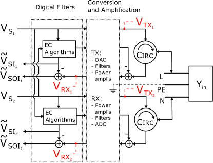
Figure 1: Proposed architecture of the full duplex PLM.

The circulator has also been proposed as hybrid coupler for IBFD PLC [16, 13]. Therefore, the same modem architecture can be used both for communication and sensing purposes.

The IBFD PLM architecture needed for the proposed system is depicted in Fig. 1. The system consists of a MIMO PLM with two transmitting and two receiving channels; the transmitting and receiving ports of each channel are connected to a circulator, which is also connected to the power line. The digital source signal $\mathbf{V_{S}}=\left[V_{S_{1}},V_{S_{2}}\right]^{T}$, where the superscript $T$ denotes the transpose operation, is converted to analog domain, thus becoming the transmitted signal $\mathbf{V_{TX}}=\mathbf{V_{S}}+\mathbf{N_{TX}}$, where $\mathbf{N_{TX}}$ is the noise introduced by the transmission chain. The circulators forward the signal to the PLN and the resulting echo is forwarded to the receiver, such that the received signal $\mathbf{V_{RX}}$ is

$$\mathbf{V_{RX}}=\mathbf{V_{SI}}+\mathbf{V_{SOI}}+\mathbf{N_{RX}}+\mathbf{N_{PL}}=\mathbf{V_{SI}}+\mathbf{V_{N}},$$ (1)

where $\mathbf{V_{SI}}$ is the echo signal, also called self interference,

$$\mathbf{V_{SI}}=-\mathbf{Y_{0}}^{-1}\bm{\rho}_{\mathbf{in}}\mathbf{Y_{0}}\mathbf{V_{TX}}\\ =-\mathbf{Y_{0}}^{-1}\bm{\rho}_{\mathbf{in}}\mathbf{Y_{0}}\mathbf{V_{S}}-\mathbf{Y_{0}}^{-1}\bm{\rho}_{\mathbf{in}}\mathbf{Y_{0}}\mathbf{N_{TX}}.$$ (2)

$\mathbf{Y_{0}}$ is the input impedance at the channel port of the circulator and $\bm{\rho}_{\mathbf{in}}$ is defined in [12, Eq. 3]. $\mathbf{V_{SOI}}$ is the PLC signal coming from a far-end ($\cdot_{FE}$), also called signal-of-interest,

$$\mathbf{V_{SOI}}=\mathbf{H}\mathbf{V_{S_{FE}}}+\mathbf{N_{TX_{FE}}}.$$ (3)

$\mathbf{N_{RX}}$ is the noise introduced by the receiver stage and $\mathbf{N_{PL}}$ is the network noise. Since $\bm{\rho}_{\mathbf{in}}$ is of interest for reflectometric sensing, it has to be estimated based on the measurement of $\mathbf{V_{RX}}$. We remark that $\mathbf{Y_{in}}$ is directly derived from $\bm{\rho}_{\mathbf{in}}$ as

$$\mathbf{Y_{in}}=\left(\mathbf{I}+\bm{\rho}_{\mathbf{in}}\right)\left(\mathbf{I}-\bm{\rho}_{\mathbf{in}}\right)^{-1}\mathbf{Y_{0}}\\ =\mathbf{Y_{0}}\left(\mathbf{V_{TX}}-\mathbf{V_{SI}}\right)\left(\mathbf{V_{TX}}+\mathbf{V_{SI}}\right)^{-1},$$ (4)

where $\mathbf{I}$ is the identity matrix.

A series of so called Echo Cancellation (EC) techniques can be used either in the analog [16] or in the digital stage [13] of the receiver to estimate $\bm{\rho}_{\mathbf{in}}$, with different accuracy based on the combination and type of algorithms used. We point out that these techniques are already used in full-duplex PLMs in the PLC context. In fact, in communications the receiver is only interested in the signal $\mathbf{V_{SOI}}$, while the echo $\mathbf{V_{SI}}$ generates a self-interference that hinders the reception of the far-end signal. Therefore, an estimate $\mathbf{\tilde{V}_{SI}}$ of $\mathbf{V_{SI}}$ is first obtained using the EC algorithms and then it is subtracted from $\mathbf{V_{RX}}$, so that the processing stage receives only $\mathbf{V_{SOI}}$ plus the network and hardware noises, as in classical half-duplex communications. In the context of network sensing, the same structure is applied, with a slight difference: $\mathbf{\tilde{V}_{SI}}$ is not only subtracted from $\mathbf{V_{RX}}$ for the communication purpose, but can also be further processed to detect and localize anomalies, as discussed in Section III.

Since the PLC channel is intrinsically linear periodic time variant (LPTV), with periodicity equal to half the mains cycle, classical EC algorithms such as the Least-Mean-Squares (LMS) would yield poor results on average. An algorithm as already been proposed that tracks channel variations in the first mains half cycle and saves the respective state (see [13, Algorithm 1]). From the second half cycle onward, a separate LMS algorithm is run for each one of the channel states. The algorithm is also able to track load impedance variations, which are identified by strong mean square error (MSE) registered both at saved or non-saved symbol indexes. In Section III, we present a novel algorithm that enables also the sensing of faults and cable degradations.

II-C End-to-end sensing

In order to sense $\mathbf{H}$, half-duplex PLMs can be used to acquire $\mathbf{V_{RX}}$ and classical estimation techniques can be used. When the transmitted signal is known, an LMS algorithm can be used to estimate $\mathbf{H}$ the same way as presented in the previous section for $\mathbf{V_{SI}}$ and $\bm{\rho}_{\mathbf{in}}$. However, transmitting known signals results in no communication between the two ends. If we want to maintain a communication link between the two modems, pilot-based or even blind CTF estimators [17] have to be used to estimate $\mathbf{H}$. The type of the transmitted signals has therefore to be chosen in order to keep a balance between high-rate communications and CTF estimation accuracy. PLC standards [18, 19] already include a number of pilot carriers in the OFDM symbols that are used to perform channel estimation. Pilots can be arranged in different ways: full pilot carriers at regular intervals (block-type), constant carrier indexes over time (comb-type) or index swapping in consecutive symbols. Block type systems have better convergence than the others in linear time invariant systems (LTI), while in the case of LPTV systems like PLC channels, comb-type or index swapping systems have been shown to yield better performance (see [20, 21] and references therein).

We finally remark that an algorithm similar to [13, Algorithm 1] can be applied to the estimation of $\mathbf{H}$ and it can be used to track periodic variations of the channel.

II-D Considerations on monitoring methods

TABLE I: Technical solutions, advantages and limitations of sensing with PLMs.

	End-to-end	Reflectometry
Solutions	Pilot-based estimation techniques	Adaptive filters based on completely known $\mathbf{V_{S}}$
Advantages	Use of common half-duplex modems	Sensing at symbol level preserving full data rate
Limitations	Sensing to the detriment of data rate	Use of more complex full-duplex modems
	Not continuous monitoring with block-type pilots	Presence of $\mathbf{V_{SOI}}$ might hinder estimation accuracy
	Not completely known $\mathbf{V_{S_{FE}}}$ with comb-type pilots	Statistics of $\mathbf{V_{S}}$ influences the estimation error

When monitoring a network, particular attention has to be payed both to the sensing signals used and the periodicity of the sensing events. Regarding the sensing signals, they influence the accuracy of the estimation of $\mathbf{H}$, $\mathbf{Y_{in}}$ or $\bm{\rho}_{\mathbf{in}}$ in different ways. In the reflectometric case the sensing signal is known, but its statistics influences the quality of the estimation [22]. In the case of end-to-end sensing, the sensing signals are represented by the pilot symbols used in communication protocols. The use of pilots intrinsically yields lower performance than knowing the sensing signal at each subcarrier, as in the reflectometric case. Hence, a lower performance in the estimation of $\mathbf{H}$ w.r.t. $\mathbf{Y_{in}}$ and $\bm{\rho}_{\mathbf{in}}$ is in general expected. Technical solutions and limitations for the reflectometric and end-to-end sensing approaches are summarized in Table I.

Regarding the periodicity of the sensing events, it depends on the convergence time of the estimation methods used and is in general a multiple of the symbol rate. The duration of an OFDM symbol in PLC is in the order of hundreds of microseconds, while the effect of the shortest anomalous events, like arching faults, lasts for some tenths of milliseconds. This means that a convergence time of tenths to hundreds of symbols is enough to capture the shortest anomalies. The status of the PLN at high frequency actually varies as often as a couple of OFDM symbols (~1 ms) due to the LPTV behavior of the channel. All these variations are tracked as explained in Section II-B and are not considered as anomalies, since they belong to the normal operation of the network.

Although using every OFDM symbol for sensing enables high resolution, it is actually needed only to sense anomalies that have no permanent effect on the system but can still be a threat, like lightning strikes, arching faults, animal or tree temporary contact with the line and others. On the other end, the anomalies that cause permanent or lasting damage to the network do not require to be sensed with such rate. In this case, $\mathbf{H}$, $\mathbf{Y_{in}}$ or $\bm{\rho}_{\mathbf{in}}$ can be estimated at time intervals that are considerably greater than the length of a communication symbol. In particular, since typical PLC systems are aware of the mains cycle period [23], we propose the following:

• sensing at symbol level is performed using the techniques presented above in order to identify temporary anomalies. We call this symbol level sensing (SLS).

• at intervals $T$ that are multiples of half the mains period, the channel is sensed using known values of both $\mathbf{V_{S}}$ and $\mathbf{V_{S_{FE}}}$ . We call this mains level sensing (MLS).

We remark that the estimation techniques used for the SLS are anyhow used anytime a PLM wants to communicate with other modems, so the overload generated by sensing is just due to the anomaly detection and location algorithm presented in Section III. Since both the end-to-end and the reflectometric SLS can track the periodic channel variations, the unperturbed situation is also periodic time-varying. Hence, the anomaly detection algorithm is run on every new sensing instance with respect to the unperturbed measurement relative to the specific sensing instant.

As for the second sensing approach, it has two main advantages: first, by sensing every $T$ mains cycles, we elude the time variations of the channel and the resulting system can be considered LTI. Second, using known signals allows us to reduce the estimation techniques to simple averaging, which would yield over a significant amount of samples toward null estimation error [24]. In fact, all the noise sources, including $\mathbf{N_{RX}}$, $\mathbf{N_{TX}}$, $\mathbf{V_{SOI}}$ and $\mathbf{N_{PL}}$, can be considered with good approximation to have mean zero.

III Anomaly detection and location

In this Section, we present an algorithm that can be used to both detect and locate anomalies, as well as distinguish between localized faults, load impedance changes and distributed faults.

III-A Anomaly detection and classification

The unperturbed situation is considered to be when, after the startup, the estimation algorithms presented in the previous section converge to a minimum estimation error. It has been shown in [15], that the noise related to the estimation of $\bm{\rho}_{\mathbf{in}}$ and $\mathbf{Y_{in}}$is zero mean if $\mathbf{V_{N}}<\mathbf{V_{S}}/10$, which is normally the case in PLN. When using adaptive algorithms, subspace or interpolation techniques with finite impulse response filters in presence of noise, the MSE is always lower bounded and positive. On the other side, the MSE tends to zero when averaging over a large sample set.

In the following, we consider the case of SLS algorithms with fixed and finite parameters, such that the MSE converges to a minimum MSE_∞. For every new estimation step $m$, we compute the quantity

$$\Delta_{sup}\left(m,n\right)=\mathbf{\tilde{A}}\left(m,n\right)-\mathbf{\tilde{A}}_{ref}\left(m,n\right)$$ (5)

or

$$\Delta_{ch}\left(m,n\right)=\mathbf{\tilde{A}}\left(m,n\right)\mathbf{\tilde{A}}_{ref}\left(m,n\right)^{-1}$$ (6)

depending on weather the chain or the superposition model for the anomaly has been chosen [12], where $\mathbf{\tilde{A}}$ stands for $\mathbf{Y_{in}}$, $\bm{\rho}_{\mathbf{in}}$ or $\mathbf{H}$, and $\mathbf{\tilde{A}}_{ref}\left(m,n\right)$ is a reference value for the unperturbed situation, chosen as a mean of the previous estimated values. If at least for one of the $n$ indexes the value of $\left|\Delta_{sup}\right|,$$\left|\Delta_{ch}\right|$ is greater than a fixed threshold (we use three times the standard deviation of $\mathbf{\tilde{A}}_{ref}\left(m,n\right)$), then the index $n_{max}$ of the maximum of (5), (6) is saved. This is because the value thus found might be caused by impulsive noise, which is common in PLNs. However, if this value is caused by an anomaly, in the following iterations a similar value will appear at $n_{max}$. In order to reduce false positives, few successive realizations of the increment against the same reference will be tested. If the value of (5), (6) at $n_{max}$ is always greater than the threshold, then an anomaly is detected. Otherwise, $\mathbf{\tilde{A}}\left(m,n\right)$ is used to update $\mathbf{\tilde{A}}_{ref}\left(m,n\right)$.

When an anomaly is detected, $\partial_{sup}(m,t)$ or $\partial_{ch}(m,t)$ are computed as the inverse Fourier transforms of (5) and (6) respectively. Their peaks are detected, either by classical peak-detection or super-resolution techniques as presented in Section III-D. The first peak of $\partial_{sup}^{Y}(m,t)$ tells already the distance of the anomaly from the receiving modem, while an ambiguity remains in the case of $\partial_{sup}^{H}(m,t)$. Regarding the type of the fault, a first distinction between localized and distributed anomalies is made. As shown in [12, Fig. 5,6], a distributed anomaly, conversely from localized anomalies, causes a shift in the peaks in frequency domain. Therefore, it is sufficient to test weather the peaks of $\mathbf{Y_{in}}$ or $\mathbf{H_{tot}}$ are also present in $\mathbf{Y_{in_{a}}}$ or $\mathbf{H_{tot_{a}}}$ respectively to understand if the anomaly is localized or distributed. In the first case, the peak would be identified in both traces, while in the second case the response will be negative. When the anomaly is identified as localized, the time domain trace is analyzed. If the position of the first peak of $\partial_{sup}(m,t)$ or $\partial_{ch}(m,t)$ coincides with the position of a peak of $\mathbf{\tilde{y}_{in}}$ or $\mathbf{\tilde{h}_{tot}}$ respectively, then the anomaly can be a load variation. To confirm this hypotesis, we look for the presence of the same peaks after the anomaly in $\mathbf{\tilde{y}_{in}}$ or $\mathbf{\tilde{h}_{tot}}$and $\mathbf{\tilde{y}_{in_{a}}}$ or $\mathbf{\tilde{h}_{tot_{a}}}$. In fact, if the anomaly is a load variation, no new peaks are created in the time domain response. If this is the case, the anomaly is identified as an impedance variation, otherwise it is a fault. The detection and classification technique is summarized in Algorithm 1.

Algorithm 1 Anomaly detection and classification algorithm

1:$\mathbf{\tilde{Y}_{in_{a}}}$, $\mathbf{\tilde{Y}_{in}}$

2:Presence of an anomaly, Type of the anomaly

3:while $\max_{n}\Delta_{sup}^{Y}<\text{thr1}$ do

4:     update $\mathbf{\tilde{A}}_{ref}$

5:     transmit a new OFDM symbol

6:     compute $\max_{n}\Delta_{sup}^{Y}$

7:end while

8:an anomaly has been detected

9:compute $\partial_{sup}^{Y}$, $\mathbf{\tilde{y}_{in_{a}}}$ and $\mathbf{\tilde{y}_{in}}$

10:compute peaks[$\partial_{sup}^{Y}$], peaks[$\mathbf{\tilde{y}_{in_{a}}}$] and peaks[$\mathbf{\tilde{y}_{in}}$]

11:compute peaks[$\mathbf{\tilde{Y}_{in_{a}}}$] and peaks[$\mathbf{\tilde{Y}_{in}}$]

12:if max{peaks[$\mathbf{\tilde{Y}_{in}}$]- peaks[$\mathbf{\tilde{Y}_{in_{a}}}$]} > thr2 then

13:     the anomaly is a distributed fault

14:else if min{peaks[$\partial_{sup}^{Y}$](1) - peaks[$\mathbf{\tilde{y}_{in}}$]} < thr3 then

15:     if max{peaks[$\mathbf{\tilde{y}_{in}}$] - peaks[$\mathbf{\tilde{y}_{in_{a}}}$]} < thr4 then

16:         the anomaly is an impedance variation

17:     else if the anomaly is a localized fault then

18:     end if

19:else

20:     the anomaly is a localized fault

21:end if

III-B Anomaly localization: one sensor

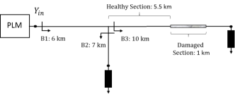
(a)

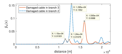
(b)

Figure 2: Example of a simple network with a damaged section: a) sketch and b) estimated admittance variation when the damaged section is on branch 2 or 3.

When just one sensor or one sensor pair (in the case of end-to-end sensing) is available, the distance of an anomaly from the measurement point can be retrieved from the position of the first peak of $\mathbf{\tilde{y}_{a}}$ or $\mathbf{\tilde{h}_{a}}$. When the topology of the network is known, the relative position of the peaks of $\mathbf{\tilde{y}_{a}}$ and $\mathbf{\tilde{h}_{a}}$ univocally relates every anomaly to a precise point in the network, enabling the localization of the anomaly. Consider the example of Fig. 2, where a network with a damaged cable section 11.5 km away from the sensing point is considered. The damaged section could be either on branch B2 or B3, but we depicted only the B3 case for simplicity. Fig. 2b shows that, if the damaged section is in branch B3, then a peak appears at 12.4 km, corresponding to the end of the damaged section and another peak appears at 15.95 km, corresponding to the position of the load at the end of the branch. On the other side, if the damaged section is in branch B2, we see a prominent peak at 12.95 km corresponding to the position of the load at the end of branch B2. This peak is actually so high that it hides the peak at 12.4 km generated by the end of the damaged section. Besides, we notice that the peaks corresponding to the network loads are located nearer to the sensing point as expected in an unperturbed situation. As explained in Section III, this is a clear sign that the detected anomaly is a distributed fault. This example shows that, in the reflectometric case, it is sufficient to analyze few peaks after the first to understand in which branch an anomaly is located. The end-to-end sensing case is more complex, as explained in [12]. In fact, the first peak of $\mathbf{\tilde{h}_{a}}$ cannot tell weather the corresponding distance is from the transmitter or the receiver; the first peak caused by a branch ending might refer to the ending towards the receiver or the transmitter, while in the reflectometric case it always refers to the farther branch ending. All of this would add significant complexity to an anomaly localization algorithm. For these reason, the anomaly localization is not treated in this work for the case of end-to-end monitoring.

The following algorithm (see Algorithm 2) can be derived to automatically locate an anomaly after it has been detected. When analyzing $\mathbf{\tilde{y}_{a}}$, its first peak provides an estimate $\hat{d}_{a}$ of the distance of the anomaly from the sensing point. If the anomaly is identified as a load impedance change, then the branch is directly identified in the hypothesis that the network is asymmetric and there are no nodes equally distant from the sensing point, which is common in PLN. If the anomaly is identified as a lumped fault or a distributed anomaly, then in a first step all the $M$ possible branches where the anomaly can be located are identified. The distance $\mathbf{d}$ between all the nodes and the receiver is also computed. Subsequently, for each of the $M$ possible branches, the difference $b$ between $\hat{d}_{a}$ and the nodes $N_{1}^{m}$ and $N_{2}^{m}$ at the extremities of the $m$th branch is computed. This step allows to identify the distance of the first few peaks after $\hat{d}_{a}$ is the fault is in branch $m$. The result is subtracted from $\mathbf{\tilde{y}_{a}}$, to check weather the guessed peaks correspond to the measurement. Finally, the branch with the lowest result is selected as the estimated anomaly branch.

Algorithm 2 Anomaly localization algorithm

1:peaks[$\partial_{sup}^{Y}$], type, topology

2:Position of the anomaly

3:$d_{an}$ = peaks[$\partial_{sup}^{Y}$](1)

4:Compute $\mathbf{d}$

5:if type == impedance variation then

6:     $a$ = find{$\mathbf{d}$ - $d_{an}$ < thr}

7:     the impedance variation is on node $a$

8:else

9:     find the M branches where the anomaly might be

10:     for i = 1 to M do

11:         compute $b$ = $\lvert\hat{d}_{a}-[N_{1}^{m},N_{2}^{m}]\rvert$

12:         compute $c$ = min{peaks[$\partial_{sup}^{Y}$]-$\left(b+\hat{d}_{a}\right)$}

13:     end for

14:     the anomaly is located on the branch with lowest $c$

15:end if

III-C Anomaly localization: multiple sensors

In the case of multiple sensors, different techniques can be applied. The simplest one is based on geometric considerations: the information about the position of the first peak of $\mathbf{\tilde{Y}_{a}}$ or $\mathbf{\tilde{H}_{a}}$ coming from multiple sensors is fused to select the point that has the expected distance from each sensor. If the network is not symmetric, two sensing points are, in the case of reflectometry, enough to univocally determine the branch where the anomaly has occurred. In the case of end-to-end sensing, the presence of multiple modems also removes the intrinsic ambiguity of the estimated distance from the receiver. We point out that two-way end-to-end sensing (i.e. a signal is transmitted from one modem to the other and a response is immediately sent back to the first one) is not sufficient to solve the position ambiguity; at least a third modem is needed.

Geometric considerations are reliable in the case of MLS, but when it comes to SLS, the anomaly needs to be localized in a short time frame, therefore all the sensors might need to perform the measurement at the same time. In this case, there is a problem of interference between the sensors, which can be alleviated by using sensing signals that are orthogonal to each other [25].

Other approaches implementable with PLMs are based on the decomposition of the time reversal operator (DORT) [26]. These approaches are specifically designed to detect and localize very weak faults along the network, but they need a simulator with a complete topological and electrical model of the network in order to work. The scattering matrix of the network is measured before and after the fault. The DORT is afterwards applied to find an optimum set of signals, whose transmission is then simulated on the test network. The energy of this optimum signals will focus on the position of the anomaly.

III-D Spectral analysis

As we explained in the previous section, locating an anomaly basically turns into finding a series of peaks in the time domain response. Due to band limitations in communication systems, especially in PLC, the resolution might not be sufficient to separate close peaks or might provide a too loose estimation of a peak position. However, when the transfer function of a system can be represented as a sum of weighted exponentials, subspace methods can be applied. This is the case of $\mathbf{H}$, $\mathbf{Y_{in}}$ or $\bm{\rho}_{\mathbf{in}}$, as explained in [12, Eq. 17, 18, 27]. Such methods are used to better detect and locate the presence of peaks, since they can achieve super-resolution [27]. In this research work, we applied different subspace algorithms [27, 28] to the anomaly localization problem. Among all, the root-Music method [28] provided the best performance. However, when many peaks have to be detected, their amplitude varies greatly, and the signal bandwidth is sufficiently wide, we found that peak-location algorithms can identify more peaks than subspace methods, even though the resolution is lower.

In the anomaly detection and localization problem it is more important to identify a peak than to precisely localize it. Therefore, peak-location algorithms are preferred in this paper over subspace algorithms.

IV Results

In this Section, we present some results obtained by simulation that show the performance in detecting and locating anomalies of the discussed algorithms.

TABLE II: Parameters used for the simulation

Parameter	Value
Frequency	4.3 kHz - 500 kHz span, 4.3 kHz sampling [18]
Network noise	According to [18, Annex D.3]
Transmitter noise	-50 dBc (10 bit DAC, OFDM [29])
Receiver noise	-60 dBc (12 bit ADC, OFDM [29])
Transmitted power	According to [18, Ch. 7]
Number of nodes	20
Average branch length	900 m [30]
Load value	According to [18, Annex D]

IV-A Simulation Setup

We developed an MTL PLN simulator using the equations presented in [12, Sec. 1]. Such simulator randomly displaces a given number of nodes on a given surface and connects them taking into account a maximum node degree (i.e. the number of branches connected to a node). If not otherwise specified, we tune the simulator to displace the nodes with average distance of 900 m, which mimics the average displacement in a low voltage distribution network, or a medium voltage underground distribution network.

An anomaly in the form of a lumped impedance or a cable branch with modified parameters can be inserted in any point of the network. The simulator computes $\mathbf{Y_{in}}$, $\mathbf{Y_{in_{a}}}$,$\bm{\rho}_{\mathbf{in}}$, $\bm{\rho}_{\mathbf{in_{a}}}$ at every node and $\mathbf{H_{tot}}$, $\mathbf{H_{tot_{a}}}$ between every node pair. As for the PLM impedance, we consider the optimum conditions for reflectometry and end-to-end transmission. In the first case, $\mathbf{Y_{0}}$ is equal to $\mathbf{Y_{C}}$ of the cable to which the PLM is branched. In the second case, the output impedance of the transmitter is fixed to 1$\Omega$ and the input impedance of the receiver is fixed to 100 k$\Omega$ as typical in half-duplex PLMs.

As for the noise and signal powers, we use standard levels for PLC as specified in [15] if not otherwise stated. We finally assume the noise introduced by the PLM coupler (hybrid and transformer) to be negligible with respect to the other noise sources.

Finally, in the following we do not make use of a specific EC algorithm in the reflectometric case or a specific interpolation filter in the end-to-end case, but we rather model the effect of the overall error when estimating $\bm{\rho}_{\mathbf{in}}$ or $\mathbf{H_{tot}}$ on the performance of the anomaly detection and location algorithms.

IV-B Comparison of models and measurement types

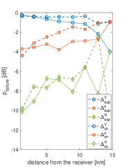
(a)

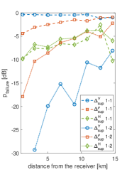
(b)

Figure 3: $p_{failure}$ when measuring $\mathbf{Y}_{\mathbf{in}}$, $\bm{\rho}_{\mathbf{in}}$ and $\mathbf{H}_{\mathbf{tot}}$. a) Comparison of the superposition and chain models, b) comparison of SISO and MIMO sensing.

As explained in Section III, there are different ways to detect the presence of an anomaly with PLMs. It is possible to estimate $\mathbf{\tilde{Y}_{in}}$, $\tilde{\bm{\rho}}_{\mathbf{in}}$ or $\mathbf{\tilde{H}_{tot}}$, using either the superposition or the chain models, which lead to the computation of $\left|\Delta_{sup}\right|$ or $\left|\Delta_{ch}\right|$ respectively. We simulated the presence of a fault in 2000 random networks and computed in each case the noise distributions of $\left|\Delta_{sup}\right|$and $\left|\Delta_{ch}\right|$ for the three considered physical quantities, both in the presence and absence of the anomaly. By integrating over the overlapping areas of the distributions, we computed the probability $p_{failure}$ of not detecting the anomaly and, vice-versa, of detecting a normal measurement as anomalous. We remark that the values of $p_{failure}$ are not important per-se, since they depend on multiple factors. Herein, we focus on the relation of the values of $p_{failure}$ obtained with different methods.

The results of Fig. 3 show $p_{failure}$ as function of $\hat{d}_{a}$ in all the aforementioned cases. Fig. 3a shows that the lowest values of $p_{failure}$ are reached when estimating $\mathbf{\tilde{H}_{tot}}$, followed by $\tilde{\bm{\rho}}_{\mathbf{in}}$ and then $\mathbf{\tilde{Y}_{in}}$, independently of the model used. This is related to the fact that the presence of anomalies yields a greater variation in $\mathbf{\tilde{H}_{tot}}$ than in $\mathbf{\tilde{Y}_{in}}$, while $\tilde{\bm{\rho}}_{\mathbf{in}}$is statistically more scattered (cfr. [12, Fig. 7]). Regarding the reliability of the models, Fig. 3a shows that the difference in $p_{failure}$ when using $\left|\Delta_{sup}\right|$ or $\left|\Delta_{ch}\right|$is not very pronounced. However, the chain model constantly yields slightly better results than the superposition model.

Fig. 3b shows the performance increment obtained when using MIMO instead of SISO measurements. We consider a fault placed between a couple of conductors in a three-wire network. The $1-1$ symbol stands for a signal that has been sent on two non-faulted conductors and received on the same pair. The $1-2$ symbol stands for a signal that has been injected on the pair of conductors interested by the fault and received on the other. The figure shows that, if the anomaly is detected using a SISO modem placed between the non-faulted conductors, $p_{failure}$ is greater than analyzing the cross-coupling transfer function with a MIMO modem. This is particularly true when considering admittance measurements, while almost no performance increment is obtained when estimating $\mathbf{\tilde{H}_{tot}}$. This result highlights the importance of using MIMO PLC modems when sensing power line networks.

IV-C Performance of the proposed algorithms

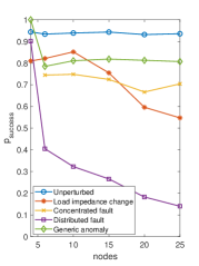
(a) Noise fixed (see Table II)

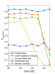
(b) 10 nodes

Figure 4: Probability of correctly detecting and identifying an anomaly.

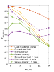
(a) Noise fixed (see Table II)

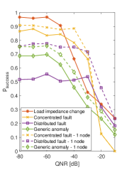
(b) 10 nodes

Figure 5: Probability of correctly locating a detected anomaly.

In this section, we evaluate the performance of Algorithm 1 and 2, focusing on the estimation of $\mathbf{\tilde{Y}_{in}}$. To this purpose, we simulate the presence of different kind of anomalies in networks of different sizes and compute the probability $p_{success}$ of correctly detecting, classifying or locating an anomaly. Moreover, in order to simulate the effect of a generic estimation algorithm, we also run a simulation where the noise parameters of Table II are no longer used. Instead, we directly set the estimation error by modifying the QNR, defined as [15]

$$QNR=\frac{\left|X_{0}\right|^{2}}{E\left[\left|X_{N}\right|^{2}\right]},$$ (7)

where $E\left[\cdotp\right]$ is the expectation operator, $X=X_{0}+X_{N}$ can be either $Y_{in}$, $\rho_{in}$, or $H_{tot}$, and the subscripts ₀ and _N stand for the mean value and the noisy component of the estimated quantity.

Fig. 4 shows the performance of Algorithm 1 for varying network size and QNR, respectively. We considered the probability of correctly detecting and classifying the unperturbed situation and the three considered anomalies. We also considered the probability of detecting a generic anomaly without classifying it. The results show that the proposed algorithm yields high values of $p_{success}$ for every kind of anomaly when the network is very small. With increasing size of the network, the performance of the concentrated fault case does not significantly change while it decreases considerably in the case of distributed faults. Fig. 4b shows that the algorithm is rather resilient to noise up to values of QNR of -30 dB, with the exception of the concentrated fault case. Low values of QNR tend not to increase the performance of the algorithm either. This suggests two observations: on one side, it is not needed to implement estimation algorithms that yield very low values of QNR; on the other side, most of the error is due to the topological structure of the network and how the detection algorithm copes with it. Therefore, better results can be achieved by improving the detection and classification algorithm.

Coming to the performance of Algorithm 2 regarding the location of anomalies, Fig. 5 shows the probability of correctly identifying the branch where an anomaly has occurred, when it has been correctly identified. In this case, both the size of the network and the QNR have a significant impact on the results. In fact, $p_{success}$ almost linearly decreases with the number of nodes and is resilient to noise only up to a QNR of around -50 dBm. The distributed fault case is more flat than the others, but this is due to the fact that the detection probability already decreases significantly with the size of the network. In Fig. 5 we also plotted the probability of identifying the first node of the branch where the anomaly has occurred (there might be more ramifications). The results are in this case significantly better, especially for the distributed fault case. This means that, even though the exact branch might not be identified, the set of possible faulted branches is significantly reduced.

Finally, we remark that the results presented in this paper refer to Algorithms 1 and 2 applied to networks with random topologies. If the algorithms had to be applied to specific topologies or topological classes, then they could be better tailored to the specific situation an yield better results.

V Conclusions

In this paper, we presented a framework to deploy power line communication modems as power grid sensors, exploiting their ability to transmit sensing signals and to acquire them. We described the modem architectures needed for sensing and evaluated different options to estimate $\mathbf{H}$, $\mathbf{Y_{in}}$ and $\bm{\rho}_{\mathbf{in}}$. We proposed two monitoring techniques, namely the symbol level sensing and mains level sensing, that allow to monitor different types of anomalies. In this regard, we proposed two algorithms that start from the estimated channel response at different time instants and are able to detect, classify and locate an anomaly. The results show that correctly identifying and locating an anomaly does not depend much on the size of the network or on the noise, but rather on the topology of the network and how it is taken into account by the detection and localization algorithms. The performance of the proposed algorithms encourages further endeavors in the area of grid monitoring with power line communications.

References

- [1] A. von Meier, E. Stewart, A. McEachern, M. Andersen, and L. Mehrmanesh, “Precision micro-synchrophasors for distribution systems: A summary of applications,” IEEE Transactions on Smart Grid, vol. 8, no. 6, pp. 2926–2936, Nov 2017.
- [2] T. Erseghe, S. Tomasin, and A. Vigato, “Topology estimation for smart micro grids via powerline communications,” Signal Processing, IEEE Transactions on, vol. 61, no. 13, pp. 3368–3377, July 2013.
- [3] M. O. Ahmed and L. Lampe, “Power line communications for low-voltage power grid tomography,” IEEE Transactions on Communications, vol. 61, no. 12, pp. 5163–5175, Dec. 2013.
- [4] A. M. Lehmann, K. Raab, F. Gruber, E. Fischer, R. Müller, and J. B. Huber, “A diagnostic method for power line networks by channel estimation of plc devices,” in 2016 IEEE International Conference on Smart Grid Communications (SmartGridComm), Nov 2016, pp. 320–325.
- [5] L. Förstel and L. Lampe, “Grid diagnostics: Monitoring cable aging using power line transmission,” in 2017 IEEE International Symposium on Power Line Communications and its Applications (ISPLC), April 2017.
- [6] F. Yang, W. Ding, and J. Song, “Non-intrusive power line quality monitoring based on power line communications,” in 2013 IEEE 17th International Symposium on Power Line Communications and Its Applications, March 2013, pp. 191–196.
- [7] M. Ahmed and L. Lampe, “Power line network topology inference using frequency domain reflectometry,” in Communications (ICC), 2012 IEEE International Conference on, June 2012, pp. 3419–3423.
- [8] F. Passerini and A. M. Tonello, “On the exploitation of admittance measurements for wired network topology derivation,” IEEE Transactions on Instrumentation and Measurement, vol. 66, no. 3, pp. 374–382, March 2017.
- [9] ——, “Power line fault detection and localization using high frequency impedance measurement,” in 2017 International Symposium on Power Line Communications and its Applications (ISPLC), April 2017.
- [10] A. Milioudis, G. Andreou, and D. Labridis, “Detection and location of high impedance faults in multiconductor overhead distribution lines using power line communication devices,” IEEE Transactions on Smart Grid, vol. 6, no. 2, pp. 894–902, March 2015.
- [11] A. M. Pasdar, Y. Sozer, and I. Husain, “Detecting and locating faulty nodes in smart grids based on high frequency signal injection,” IEEE Transactions on Smart Grid, vol. 4, no. 2, pp. 1067–1075, June 2013.
- [12] F. Passerini and A. M. Tonello, “Smart grid network sensing using power line modems: Effect of anomalies on signal propagation,” Submitted to IEEE Transactions on Smat Grids, 2018, available on arXiv.
- [13] G. Prasad, L. Lampe, and S. Shekhar, “In-band full duplex broadband power line communications,” IEEE Transactions on Communications, vol. 64, no. 9, pp. 3915–3931, Sept 2016.
- [14] L. Lampe, A. M. Tonello, and T. G. Swart, Eds., Power Line Communications: Principles, Standards and Applications from Multimedia to Smart Grid. Wiley, 2016.
- [15] F. Passerini and A. M. Tonello, “Analysis of high-frequency impedance measurement techniques for power line network sensing,” IEEE Sensors Journal, vol. 17, no. 23, pp. 7630–7640, Dec 2017.
- [16] ——, “Adaptive hybrid circuit for enhanced echo cancellation in full duplex PLC,” in 2018 IEEE International Symposium on Power Line Communications and its Applications (ISPLC), April 2018.
- [17] A. Musolino, M. Raugi, and M. Tucci, “Cyclic short-time varying channel estimation in OFDM power-line communication,” IEEE Transactions on Power Delivery, vol. 23, no. 1, pp. 157–163, Jan 2008.
- [18] IEEE Standard for Low-Frequency (less than 500 kHz) Narrowband Power Line Communications for Smart Grid Applications. IEEE 1901.2-2013, 2013.
- [19] IEEE Standard for Broadband over Power Line Networks: Medium Access Control and Physical Layer Specifications. IEEE 1901-2010, 2010.
- [20] A. A. M. Picorone, T. R. Oliveira, and M. V. Ribeiro, “PLC channel estimation based on pilots signal for ofdm modulation: A review,” IEEE Latin America Transactions, vol. 12, no. 4, pp. 580–589, June 2014.
- [21] S. Coleri, M. Ergen, A. Puri, and A. Bahai, “Channel estimation techniques based on pilot arrangement in ofdm systems,” IEEE Transactions on Broadcasting, vol. 48, no. 3, pp. 223–229, Sep 2002.
- [22] S. Haykin, Adaptive Filter Theory (3rd Ed.). Upper Saddle River, NJ, USA: Prentice-Hall, Inc., 1996.
- [23] H. A. Latchman, S. Katar, L. W. Yonge, and S. Gavette, Homeplug AV and IEEE 1901: A Handbook for PLC Designers and Users. John Wiley & Sons, Inc., 2013. [Online]. Available: http://dx.doi.org/10.1002/9781118527535
- [24] S. Kay, Fundamentals of Statistical Signal Processing - Estimation Theory. Prentice-Hall, 1993.
- [25] A. Lelong, L. Sommervogel, N. Ravot, and M. O. Carrion, “Distributed reflectometry method for wire fault location using selective average,” IEEE Sensors Journal, vol. 10, no. 2, pp. 300–310, Feb 2010.
- [26] M. Kafal, A. Cozza, and L. Pichon, “Locating multiple soft faults in wire networks using an alternative dort implementation,” IEEE Transactions on Instrumentation and Measurement, vol. 65, no. 2, pp. 399–406, Feb 2016.
- [27] P. Stoica and R. Moses, Spectral Analysis of Signals. Pearson Prentice Hall, 2005. [Online]. Available: https://books.google.at/books?id=h78ZAQAAIAAJ
- [28] A. Barabell, “Improving the resolution performance of eigenstructure-based direction-finding algorithms,” in ICASSP ’83. IEEE International Conference on Acoustics, Speech, and Signal Processing, vol. 8, Apr 1983, pp. 336–339.
- [29] C. R. Berger, Y. Benlachtar, R. I. Killey, and P. A. Milder, “Theoretical and experimental evaluation of clipping and quantization noise for optical ofdm,” Opt. Express, vol. 19, no. 18, pp. 17 713–17 728, Aug 2011. [Online]. Available: http://www.opticsexpress.org/abstract.cfm?URI=oe-19-18-17713
- [30] G. A. Pagani and M. Aiello, “Power grid network evolutions for local energy trading,” 2012. [Online]. Available: https://arxiv.org/abs/1201.0962