Robust parameter determination in epidemic models with analytical descriptions of uncertainties

Abstract

Compartmental equations are primary tools in disease spreading studies. Their predictions are accurate for large populations but disagree with empirical and simulated data for finite populations, where uncertainties become a relevant factor. Starting from the agent-based approach, we investigate the role of uncertainties and autocorrelation functions in SIS epidemic model, including their relationship with epidemiological variables. We find new differential equations that take uncertainties into account. The findings provide improved predictions to the SIS model and it can offer new insights for emerging diseases.

Communicable diseases are health disorders caused by pathogens transmitted from infected individuals to susceptible ones Bonita et al. (2006). In general, the transmission process occurs with variable success rate, subjected to stochastic uncertainties during the infectious period of the host. These uncertainties comprehend aspects related to transmission mechanisms and availability of adequate contact between hosts and susceptible individuals. The latter aspect has been further improved via network theory, accounting for more realistic social interactions and highlighting the role of central hubs in general disease spreading dynamics Albert and Barabási (2002); Pastor-Satorras et al. (2015); Eames and Keeling (2002); Keeling and Eames (2005); Bansal et al. (2007). For large and well-connected populations, stochastic factors are discarded in favor of differential equations, also known as compartmental equations Kermack and McKendrick (1927). Generalizations for compartmental equations have been able to reproduce pandemics and extract relevant characteristics, taking into account more complex network topologies Pastor-Satorras et al. (2015); Pastor-Satorras and Vespignani (2001a, b); Chen et al. (2017).

In contrast, the stochastic nature of disease transmission cannot be omitted for a number of scenarios. It becomes more pronounced for small populations. In this case, the individual characteristics of each agent forming the population are relevant variables to the spreading process. Incidentally, this is often the case of emerging diseases Heesterbeek et al. (2015). Because the population cannot be treated as homogeneous, average values for the population are no longer adequate and the accuracy of compartmental equations decreases for increasing uncertainties. Stochastic models deal with this issue by proposing simpler rules to express the disease transmission, taking the relevant stochastic factors into account. Besides average values, stochastic models possess additional tools to provide further insights, including autocorrelation functions. For instance, in the standard Brownian motion, the delta-like behavior observed for the white-noise autocorrelation function dictates the linear dependence between spatial variance and time. In disease spreading processes, however, autocorrelation functions have been largely neglected.

Here, we study the role of uncertainties and the normalized autocorrelation function, $D_{\rho\rho}(t)$, in the SIS epidemic model for a population with $N$ agents. From $D_{\rho\rho}(t)$, we derive the differential equation that governs the dynamics of the variance $\sigma^{2}(t)$ associated with the average density of infected agents $\langle\rho(t)\rangle$ in the population. We build a system of differential equations to describe the SIS model and validate them with numerical simulations. In addition, we briefly discuss the manner in which the Fano factor affects the extraction of epidemiological parameters.

Compartmental models. Let $\rho(t)$ be the density of infected agents in a population of size $N$ in the SIS model. In the compartmental approach, the population is assumed to be large, homogeneous and highly interconnected. As a result, agents can be regarded as statistically equivalent. This implicit assumption is equivalent to complete the permutation symmetry, which is also found in the complete graph Albert and Barabási (2002). Thus, $\rho(t)$ becomes the key variable in the compartmental approach.

The other relevant assumption concerns the transmission mechanism. Because the population is taken as homogeneous, the adequate interaction between infected and susceptible agents occurs with probability proportional to $(1-\rho)\rho$. This assumption constitutes the basis for the random mixing hypothesis Keeling and Eames (2005). At the same time, recovery events are proportional to the infected density $\rho$. Adding both contributions, the SIS compartmental equation for infected density is written as

$$\frac{d\rho}{dt}=\alpha\left(1-\rho\right)\rho-\gamma\rho,$$ (1)

where $\alpha$ and $\gamma$ are the transmission and recovery rate, respectively. A well-accepted generalization proposed in Ref. Pastor-Satorras and Vespignani (2001a) takes network metrics into account in the transmission rate, improving the overall accuracy of Eq. (1) for complex networks Pastor-Satorras et al. (2015).

Rearranging Eq. (1), we obtain

$$\frac{d}{dt}\ln\rho=\alpha(\rho_{\textrm{eq}}-\rho),$$ (2)

where $\rho_{\textrm{eq}}=1-\gamma/\alpha$ is the steady state density for $\alpha>\gamma$. From Eq. (2), one can extract $\alpha$ and $\gamma$ by a linear fit. Furthermore, using the actual solution of Eq. (1) in Eq. (2) leads to:

$$\frac{1}{\rho}\frac{d}{dt}\ln\rho={\alpha}\left[\frac{\rho_{\textrm{eq}}}{\rho(0)}-1\right]\textrm{e}^{-\alpha\rho_{\textrm{eq}}t},$$ (3)

whose decay rate depends only on epidemiological parameters.

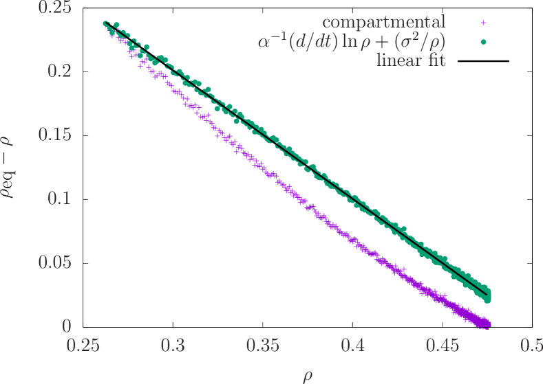
Figure 1: Deviations of compartmental predictions. Values of $\rho_{\textrm{eq}}-\rho$ versus $\rho$ using the formula from compartmental equation $(d/dt)\ln\rho$ without corrections (cross), with corrections that depend on Fano factor $\sigma^{2}/\rho$ (full circle). MC simulations are performed using $10^{6}$ samples for complete graph with $N=50$ agents, $\gamma=1/2$ and $\alpha=1$. Linear fit (solid line) produces $\gamma_{\textrm{data}}=0.50(3)$ and $\alpha_{\textrm{data}}=1.00(0)$.

It should be clear by now that Eq. (1) is an important tool to extract epidemiological parameters. What would be the implications for epidemiological studies if Eq. (1) had additional terms or corrections? The current methodology to evaluate $\alpha$ and $\gamma$ would carry systematic errors. Fig. (1) displays the values of $\alpha^{-1}(d/dt)\ln\rho$ using Eq. (2) obtained from numerical simulations. It deviates from $\rho_{\textrm{eq}}-\rho$. Even more, parameter estimation for $\rho$ that is typical during the onset of epidemics underestimates the transmission rate. If the Fano factor is taken into account, however, we recover the linear behavior, as we discuss in what follows.

Agent-based models. In the stochastic approach, the population consists of $N$ distinguishable agents connected to each other according to a pre-defined adjacency matrix $A$ ($N\times N$). In the complete graph, each agent interacts with the remaining $N-1$ agents, $A_{ij}=1-\delta_{ij}$. Each agent ($k=0,1,\ldots,N-1$) may assume one of two possible health states $n_{k}$ in the SIS model, either susceptible ($n_{k}=0$) or infected ($n_{k}=1$). Following Ref. Nakamura et al. (2017), there are $2^{N}$ available configurations in the canonical basis $\lvert\mu\rangle$, with $\mu=0,1,\ldots,2^{N-1}$. Configurations are readily extracted from the binary construction $\mu=n_{0}2^{0}+n_{1}2^{1}+\cdots+n_{N-1}2^{N-1}$. As an example, for $N=4$, the configuration $\lvert 0\rangle=\lvert 0000\rangle$ represents the infected-free configuration, whereas all agents are infected in $\lvert 15\rangle=\lvert 1111\rangle$.

In this paper, we treat the disease spreading process as a Markov process. Following Ref. Nakamura et al. (2017), the master equation in operator notation is

$$\frac{d}{dt}\lvert P(t)\rangle=-\hat{H}\lvert P(t)\rangle,$$ (4)

in which $\lvert P(t)\rangle=\sum_{\mu=0}^{2^{N}-1}P_{\mu}(t)\lvert\mu\rangle$ is the probability vector, with $P_{\mu}(t)$ being the instantaneous probability to find the system in the configuration $\lvert\mu\rangle$; and $\hat{H}$ is the generator of time translations, given by the following expression:

$$\hat{H}=\frac{\alpha}{N}\sum_{k,\ell=0}^{N-1}A_{k\ell}(1-\hat{n}_{k}-\hat{\sigma}_{k}^{+})\hat{n}_{\ell}+\gamma\sum_{k=0}^{N-1}(\hat{n}_{k}-\hat{\sigma}^{-}_{k}).$$ (5)

The operators $\hat{n}_{k}$ extract the health state of the $k$-th agent, $\hat{n}_{k}\lvert n_{0}\cdots n_{k}\cdots\rangle=n_{k}\lvert n_{0}\cdots n_{k}\cdots\rangle$, while $\hat{\sigma}_{k}^{\pm}$ are the usual spin-$1/2$ ladder operators. Operators are assigned the hat symbol to distinguish them from scalars.

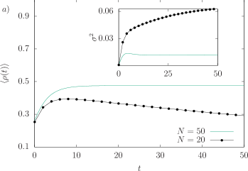
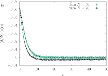
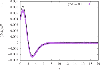
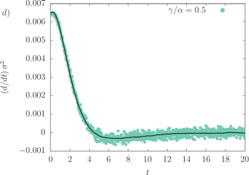
Figure 2: Uncertainty in agent-based simulations. a) Density of infected agents for $10^{6}$ simulations, with $\gamma/\alpha=1/2$, and $N=20$ (full circle) or $N=50$ (solid line) agents. The curve with $N=50$ is compatible with compartmental equations, while $\langle\rho(t)\rangle$ decays for the case with $N=20$ agents. (Inset) Uncertainties become more prominent in smaller populations, suggesting finite size corrections. b) Temporal derivative of $\langle\rho\rangle$ using formula in Eq. (7) (dashed lines) and their corresponding values calculated directly from data (circles). c) Forward time derivative of $\sigma^{2}(t)$ for $N=50$ agents and $\gamma/\alpha=0.1$ (circles). The solid line represents the values extracted using Eq. (8). Same as c) but $\gamma/\alpha=1/2$.

Eqs. (4) and (5) can be used to evaluate the average density of infected agents,

$$\langle\rho(t)\rangle\equiv\frac{1}{N}\sum\limits_{\mu=0}^{2^{N}-1}\eta_{\mu}P_{\mu}(t),$$ (6)

where $\eta_{\mu}\equiv\sum_{k}\langle\mu|\hat{n}_{k}|\mu\rangle$ is the number of infected agents in the configuration $\lvert\mu\rangle$. Exploiting the fact that $\sum_{\mu}\eta_{\mu}\langle\mu|\sum_{k}\hat{\sigma}^{+}_{k}|\nu\rangle=(\eta_{\nu}+1)(N-\eta_{\nu})$ and $\sum_{\mu}\eta_{\mu}\langle\mu|\sum_{k}\hat{\sigma}_{k}^{-}|\nu\rangle=(\eta_{\nu}-1)\eta_{\nu}$, in the complete graph,

$$\frac{d\langle\rho\rangle}{dt}=\alpha\left[\rho_{\textrm{eq}}-\langle\rho(t)\rangle\right]\langle\rho(t)\rangle-\alpha\sigma^{2}(t),$$ (7)

with instantaneous variance $\sigma^{2}(t)=\langle\rho^{2}\rangle-\langle\rho\rangle^{2}$. Eq. (7) exhibits excellent agreement with numerical simulations (see Fig. 1), and recovers the compartmental equation Eq. (1) for vanishing $\sigma^{2}(t)$. Fig. 2 depicts $\langle\rho(t)\rangle$ in the complete graph for $N=20$ and $50$ agents. The case with $N=20$ deviates from compartmental results: fluctuations that eradicate the disease are more likely to occur in scenarios with small populations, even if agents are statistically equivalent.

We emphasize that the inherent fluctuations of the disease spreading process is summarized by $\sigma^{2}(t)$ in Eq. (7). An initial uncertainty evolves during the time evolution of $\rho(t)$, reinforced by the fact that agents can only be either susceptible or infected, i.e., they obey Fermi-Dirac statistics. In a sense, $\sigma^{2}(t)$ is conceptually similar to the shot noise in condensed matter physics Blanter and Büttiker (2000).

As the plots of Fig. 2 show, numerical simulations support Eq. (7) predictions with good accuracy, highlighting the role of uncertainties in the SIS model. Noting that $\sigma^{2}(t)$ depends on time, there must exist an additional differential equation for $\sigma^{2}(t)$ (see Fig. 2). Indeed, the same rationale behind Eq. (7) can be used to find $(d/dt)\sigma^{2}$:

$$\frac{1}{2\alpha}\frac{d\sigma^{2}}{dt} =\left[\langle\rho\rangle+\rho_{\textrm{eq}}-\frac{1}{N}\right]\sigma^{2}(t)-\left[\langle\rho^{3}\rangle-\langle\rho\rangle^{3}\right]+$$

$$-\left[\frac{\langle\rho\rangle+\rho_{\textrm{eq}}}{2}-1\right]\frac{\langle\rho\rangle}{N}.$$ (8)

Even if $o(1/N)$ corrections are omitted, one still must take into account the contributions from $\Delta_{3}(t)\equiv\langle\rho^{3}\rangle-\langle\rho\rangle^{3}$. Formally, we could calculate the differential equation for $\Delta_{3}(t)$ but then we would have to deal with $\langle\rho^{4}(t)\rangle$ and so on.

Let us briefly assume that is possible to estimate $\Delta_{3}(t)$ without higher statistical moments. In this case, Eqs. (7) and (8) form a system of differential equations for $\rho(t)$ and $\sigma^{2}(t)$. Therefore, our main task is to obtain surrogate dynamics for $\Delta_{3}(t)$, which likely depend on the behavior or nature of the fluctuation itself. In fact, the density autocorrelation function provides valuable insights on $\Delta_{3}(t)$ for non-symmetric fluctuations. Likewise, the existing relationship between $\Delta_{3}(t)$ and the instantaneous coefficient of skewness, $\kappa_{3}(t)$, provides a way to investigate symmetric fluctuations.

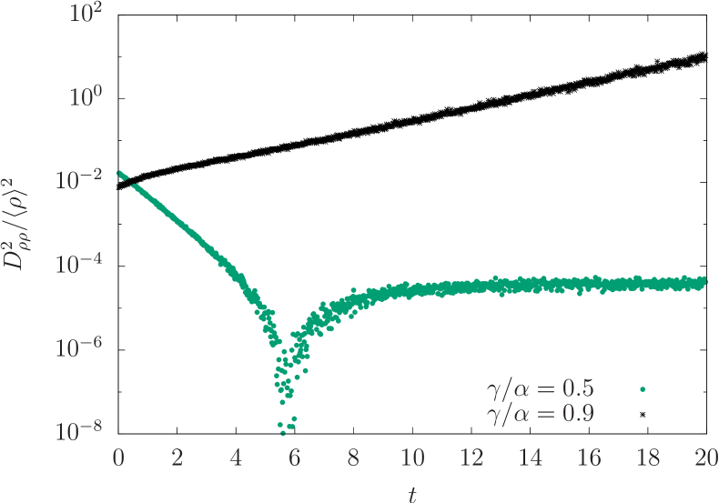
Figure 3: Contributions for $|D_{\rho\rho}(t)/\langle\rho\rangle|^{2}$. Simulations results comprehend $10^{6}$ simulation samples in the complete graph with $N=50$. Gaussian fluctuations are present for $\gamma/\alpha=0.5$ (green circles). An exponential decay is observed during the outbreak onset. The divergence appears as $\langle\rho\rangle$ approaches $\rho_{\textrm{eq}}$. Finite size corrections drive $\langle\rho(\infty)\rangle$ to slightly lower values than $\rho_{\textrm{eq}}$ in the steady state. Non-Gaussian fluctuations and finite size effects create exponential growth for $\gamma/\alpha=0.9$ (black cross).

Autocorrelation function. For typical disease spreading processes, the correlations between the various agents that comprise the finite system are usually weak. So it might seem counterintuitive to assume that correlations are relevant statistics in epidemic models. However, autocorrelation functions and variances share similar magnitudes. Therefore, there is no ground to discard one and keep the other unless proven otherwise.

Let $C_{\rho\rho}(t)$ be the instantaneous autocorrelation function between $\rho(t)$ and $\rho(t+\delta t)$, lagged by a single time window:

$$C_{\rho\rho}(t)\equiv\langle\rho(t+\delta t)\rho(t)\rangle-\langle\rho(t)\rangle^{2}.$$ (9)

Here, averages are evaluated by considering samples from an ensemble instead of usual Fourier transform, as the ergodic hypothesis is unavailable. For Markov processes,

$$\langle\rho(t+\delta t)\rho(t)\rangle=\frac{1}{N^{2}}\sum_{\mu}\sum_{k,j}\langle\mu|\hat{n}_{k}\textrm{e}^{-\hat{H}\delta t}\hat{n}_{j}|P(t)\rangle.$$ (10)

The evaluation of this expression involves the same rationale used for Eq. (7). Plugging the result into Eq. (9) we find the relation between $\langle\rho^{3}(t)\rangle$ and $C_{\rho\rho}(t)$, namely, $C_{\rho\rho}(t)-\sigma^{2}(t)=\alpha\delta t\left[\rho_{\textrm{eq}}(\langle\rho\rangle^{2}+\sigma^{2})-\langle\rho^{3}\rangle\right]+o(\delta t^{2})$. Unfortunately, $C_{\rho\rho}(t)$ does not exhibit a simple functional form.

Instead, consider the normalized autocorrelation function:

$$D_{\rho\rho}(t)\equiv\alpha\left[\rho_{\textrm{eq}}-\frac{\langle\rho^{3}\rangle}{\langle\rho\rangle^{2}}\right]+\alpha\rho_{\textrm{eq}}\frac{\sigma^{2}}{\langle\rho\rangle^{2}}.$$ (11)

Note that $D_{\rho\rho}(t)$ recovers Eq. (2) when $\sigma^{2}\rightarrow 0$ and $N\rightarrow\infty$: $D_{\rho\rho}(t)\rightarrow\alpha[\rho_{\textrm{eq}}-\langle\rho(t)\rangle]$. Hence $D_{\rho\rho}(t)$ can be interpreted as an alternative metric to describe the evolution of the system. We can explore this interpretation to learn more about $D_{\rho\rho}(t)$ and its time dependence. For instance, using Eq. (3) as inspiration, $D_{\rho\rho}(t)/\langle\rho(t)\rangle$ exhibits exponential behavior during transient regimes (see Fig. 3) regardless of fluctuation type. Thus, $D_{\rho\rho}(t)$ is a suitable quantity to express $\Delta_{3}(t)$ in Eq. (8):

$$\frac{1}{2\alpha}\frac{d}{dt}\ln\sigma^{2}=\langle\rho\rangle+\left[\langle\rho\rangle-{\rho_{\textrm{eq}}}+\frac{1}{\alpha}{D_{\rho\rho}}\right]\frac{\langle\rho\rangle^{2}}{\sigma^{2}}+\frac{s}{N},$$ (12)

with finite size contributions $s(t)\equiv s=(\rho/2\sigma^{2})(2-\rho-\rho_{\textrm{eq}})-1$.

We can gain further insights about $D_{\rho\rho}(t)$ in the case in which the variance remains finite but $\langle\rho(t)\rangle$ decays exponentially with decay rate $\tau$. Because $\sigma^{2}(t)$ is finite, there exists $\varepsilon>0$ such that $\sigma^{2}(t)<\varepsilon$ for any $t$. Therefore, $\sigma^{2}/\langle\rho\rangle^{2}\sim\varepsilon\,\textrm{e}^{2t/\tau}$ increases exponentially. This observation hints about the general behavior of $D_{\rho\rho}(t)$: the magnitude of $D_{\rho\rho}(t)$ should also increase exponentially. We summarize these observations by measuring $|D_{\rho\rho}/\langle\rho\rangle|^{2}$. Fig. 3 shows the striking differences between symmetric and non-symmetric fluctuations. More importantly, for non-symmetric fluctuations,

$$D_{\rho\rho}(t)\approx-\alpha D_{1}\,\textrm{e}^{t/\tau}\langle\rho(t)\rangle$$ (13)

provides a convenient description for the normalized autocorrelation function, with fitting parameters $D_{1}$ and $\tau$. We remark that the exponential fitting in Eq. (13) deviates from data values at the very beginning of the outbreak (see Fig. 3), so there is still room for improvements especially for more complex population structures.

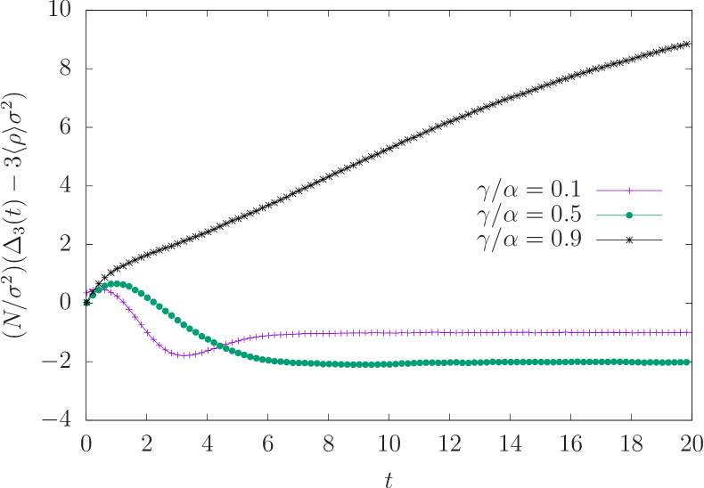
Figure 4: Deviations from Gaussian behavior. Simulations are performed in the complete graph with $N=50$ agents, and $10^{6}$ samples. The quantity $\Delta_{3}-\Delta_{3}^{\textrm{gauss}}=\sigma^{2}\kappa_{3}$ measures the deviation of the system compared to Gaussian fluctuations. Curves for $\gamma/\alpha=0.1$ and $0.5$ imply $\kappa_{3}\sim o(1/N)$. This behavior is not observed for $\gamma/\alpha=0.9$. Error bars omitted.

Gaussian fluctuations. For large population sizes, stochastic effects are entirely dominated by finite second moments and are well represented by Gaussian fluctuations. Because they are distributed according to a symmetric probability distribution function, their coefficient of skewness vanishes, $\kappa_{3}(t)=0$. Noting that $\kappa_{3}=(\Delta_{3}-3\langle\rho\rangle\sigma^{2})/\sigma^{3}$, we conclude that $\Delta_{3}^{\textrm{gauss}}\approx 3\langle\rho(t)\rangle\sigma^{2}(t)$ for Gaussian fluctuations. Indeed, Fig. 4 shows the ansatz is not too far fetched since $\Delta_{3}(t)-\Delta_{3}^{\textrm{gauss}}(t)\sim o(\sigma^{2}/N)$ for ratios $\gamma/\alpha=0.1$ and $0.5$, but not for $\gamma/\alpha=0.9$, which according to Fig. 4 are dominated by non-gaussian fluctuations.

Ignoring $o(1/N)$ corrections in Eq. (8), we write the following differential equations:

$$\frac{1}{\alpha}\frac{d}{dt}\ln\langle\rho\rangle =\rho_{\textrm{eq}}-\langle\rho\rangle-\frac{\sigma^{2}}{\langle\rho\rangle},$$ (14a)

$$\frac{1}{2\alpha}\frac{d}{dt}\ln\sigma^{2} =\rho_{\textrm{eq}}-2\langle\rho\rangle,$$ (14b)

valid under the assumption $N\rightarrow\infty$. We can draft an immediate observation from Eq. (14b). As long as the $\sigma^{2}(0)>0$, uncertainties play a role in the SIS epidemic model. Conversely, $\sigma^{2}(0)=0$ implies $\sigma^{2}(t)=0$ and warrants the validity of Eq. (2). In addition, we see that the instantaneous Fano factor $\sigma^{2}(t)/\langle\rho(t)\rangle$ in Eq. (14a) improves compartmental predictions if $\sigma^{2}$ remains finite. However, it also emphasizes that uncertainties rather than $\rho(t)$ drive the disease spreading in the low-density regimes.

Despite the insights provided by Eqs. (14a) and (14b), there are still some remaining issues. The most relevant issue deals with estimates for $\sigma^{2}(0)$ from epidemiological data. This issue can be avoided entirely by combining the system of differential equations into a single differential equation (angular brackets dropped for simplicity):

$$\frac{d^{2}\rho}{dt^{2}}=3\alpha\left(\rho_{\textrm{eq}}-2\rho\right)\left[\frac{d\rho}{dt}-\frac{2\alpha}{3}(\rho_{\textrm{eq}}-\rho)\rho\right].$$ (15)

This equation shares the same steady state solution as Eq. (1). The major difference occurs during the transient regime: uncertainties introduced by Gaussian fluctuations slowdown the system.

Conclusion. We investigate the effects of uncertainties to disease spreading and their implications in the SIS epidemic model. We derive stochastic equations for $\rho(t)$ and $\sigma^{2}(t)$ by introducing surrogate dynamics for symmetric and non-symmetric fluctuations. Our findings reconcile the simplicity of canonical compartmental equations with the accuracy of agent-based simulations, thus creating suitable tools for practitioners of Epidemiology and related fields. At the core of this research, we demonstrate that uncertainty cannot be neglected in the SIS epidemic model in finite populations, even when the population is large and comprised of statistically equivalent agents. For non-symmetric fluctuations, the normalized autocorrelation function can be parametrized, providing again a closed system for the variables $\langle\rho(t)\rangle$ and $\sigma^{2}(t)$. The special case of Gaussian fluctuations provides additional simplifications from which we derive a second-order differential equation for $\langle\rho(t)\rangle$. Finally, we stress that this research evaluates the impact of uncertainties only for homogeneous populations. As a consequence, connections between agents are described according to the complete graph. An intriguing question that arises is whether the inherent uncertainties associated with network metrics influence or enhance fluctuations in the disease spreading. For instance, scale-free networks contain uncertainties that scale with $N$, which in turn must contribute in the master equation Eq. (4).