DESY 18-117, DO-TH 18/15
The $\rho$ parameter at three loops and elliptic integrals

Abstract:

We describe the analytic calculation of the master integrals required to compute the two-mass three-loop corrections to the $\rho$ parameter. In particular, we present the calculation of the master integrals for which the corresponding differential equations do not factorize to first order. The homogeneous solutions to these differential equations are obtained in terms of hypergeometric functions at rational argument. These hypergeometric functions can further be mapped to complete elliptic integrals, and the inhomogeneous solutions are expressed in terms of a new class of integrals of combined iterative non-iterative nature.

1 Introduction

The calculation of multi-loop Feynman integrals constitutes a crucial step required for the computation of quantum corrections to different standard model processes occurring at the LHC and other collider experiments. Considerable progress has been made in this regard in the past few decades, and many Feynman integrals have been computed using a variety of methods. In particular, integration by parts identities (IBP) have been used to express all required Feynman integrals in terms of a small set of so called master integrals [2]. The master integrals can then be calculated by taking their derivatives with respect to the invariants of the problem, which leads to an expression that can be rewritten in terms of the master integrals themselves by inserting the IBPs. This leads to a system of differential equations for the master integrals, which can be decoupled and, given appropriate boundary conditions, one may then try to solve [3]. In many cases, the decoupled equations turn out to be first order factorizable, and the master integrals can be expressed in terms of iterated integrals, such as the harmonic polylogarithms [4], Kummer-Poincaré iterated integrals [5, 6], cyclotomic polylogarithms [7], and iterated integrals with squared-root-valued letters in the alphabet [8], among others [9]. Also associated nested sum representations are obtained [10, 6, 8, 9] and special constants appear in these representations, see e.g. [11].

There are many physical problems that have been solved entirely in terms of these types of functions, particularly, problems involving only massless particles or planar Feynman diagrams. On the other hand, when trying to solve problems involving massive particles and/or non-planar diagrams, one may encounter Feynman integrals for which the corresponding differential equation turns out not to be first order factorizable, cf. [12, 13, 14, 15, 16, 17, 18, 19, 20, 21, 22, 23, 24, 25, 26, 27, 28, 29, 30, 31, 32, 33, 34, 35, 36, 37, 38, 39, 40, 41, 42, 43, 44]. Feynman integrals obeying differential equations that can be factorized to first order, except for one irreducible term of second order, represent the next level of complexity among the integrals arising in many problems of interest in perturbative calculations. One such problem turns out to be the two-mass three-loop corrections to the $\rho$ parameter. This problem is ideal for the study of the computation of this type of Feynman integrals because it has a particularly nice feature, namely, the master integrals for which the differential equations contain a term of second order are almost the last ones that need to be solved. Other problems, which require the solutions of master integrals such as the sunrise or the kite integrals [12, 13, 14, 15, 16], can be more cumbersome, since these integrals are usually the first ones that need to be solved and their solutions reappear throughout the rest of differential equation system, with new integrations over these solutions at each step. The fact that this does not happen in the case of the two-mass three-loop contributions to the $\rho$ parameter means that it is simpler to obtain a fully analytic result for the physical quantity.

The $\rho$ parameter is an important quantity in the standard model [45] that measures the relative strength between the neutral current and charged current interaction and is given by

$$\rho=\frac{M_{W}^{2}}{M_{Z}^{2}\cos^{2}(\theta_{W})}~{},$$ (1)

which at tree level is equal to 1, and receives quantum corrections

$$\rho=1+\Delta\rho,$$ (2)

given by

$$\Delta\rho=\frac{\Sigma_{Z}(0)}{M_{Z}^{2}}-\frac{\Sigma_{W}(0)}{M_{W}^{2}},$$ (3)

where $\Sigma_{Z}(0)$ and $\Sigma_{W}(0)$ are the transverse parts of the $Z$ and $W$ boson propagators, respectively, which are defined by

$$\Sigma_{W/Z}(0)=\frac{g_{\mu\nu}}{d}\Pi_{W/Z},$$ (4)

where $\Pi_{W/Z}$ are the corresponding polarization functions. The quantum loop corrections as an expansion in the strong coupling constant $\alpha_{s}$ can be written as

$$\Delta\rho=\frac{3G_{F}m_{t}^{2}}{8\pi^{2}\sqrt{2}}\biggl{(}\delta^{(0)}+\frac{\alpha_{s}}{\pi}\delta^{(1)}+\left(\frac{\alpha_{s}}{\pi}\right)^{2}\delta^{(2)}+{\cal O}(\alpha_{s}^{3})\biggr{)}.$$ (5)

Some of the most recent computations of these quantum corrections can be found in [46, 47, 48, 49, 50, 51]. In the calculation of the two-mass contribution to the three-loop term $\delta^{(2)}$ presented in [51], it was found that all but six of the master integrals required to obtain this quantity could be computed in terms of harmonic polylogarithms depending on the ratio of the two masses,

$$x=\frac{m_{1}}{m_{2}},\quad\quad m_{1}<m_{2}\quad\Rightarrow\quad 0<x<1.$$ (6)

The remaining six master integrals are depicted in Figure 1, and can be expanded up to order $\varepsilon^{0}$ (the calculation is done using dimensional regularization, where the dimension $D$ is given by $D=4-2\varepsilon$) as follows

$$J_{k}^{(3)}(x)=\frac{1}{\varepsilon^{3}}g_{k,-3}(x)+\frac{1}{\varepsilon^{2}}g_{k,-2}(x)+\frac{1}{\varepsilon}g_{k,-1}(x)+f_{k}(x)+{\cal O}(\varepsilon)\,,$$ (7)

where $k$ labels the different master integrals. We use the same notation as the authors of Ref. [51], i.e., in the case of the six master integrals under consideration, $k\in\{8a,8b,9a,9b,10a,10b\}$. It turns out that the pole terms $g_{k,-i}$ ($i=1,2,3$) of these six master integrals can also be expressed entirely in terms of harmonic polylogarithms in the variable $x$, while the constant terms $f_{k}$ obey a non-factorizable second order differential equation in the case of $k\in\{8a,8b,9a,9b\}$, and in the case of $k\in\{10a,10b\}$ we have a first order differential equation where the previous integrals appear in the inhomogeneities.

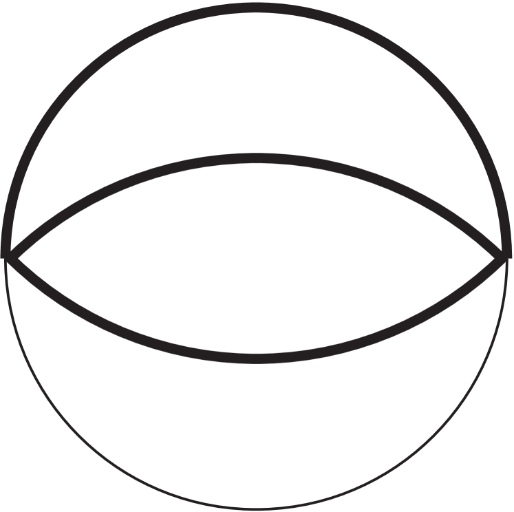
$J^{(3)}_{8a}$

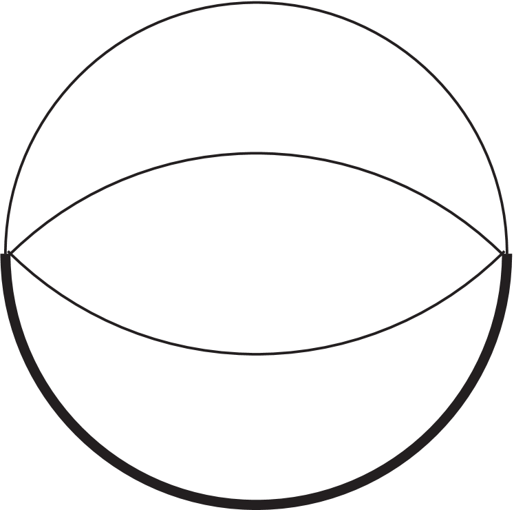
$J^{(3)}_{8b}$

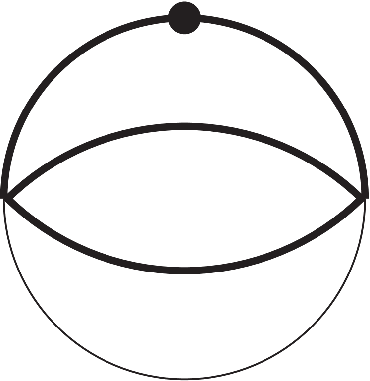
$J^{(3)}_{9a}$

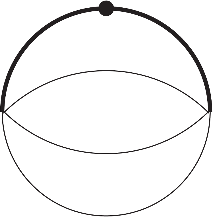
$J^{(3)}_{9b}$

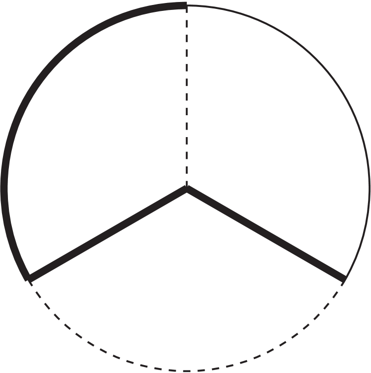
$J^{(3)}_{10a}$

$J^{(3)}_{10b}$

Figure 1: The six master integrals required for the calculation of the two-mass three-loop contributions to the $\rho$ parameter which obey differential equations that are not factorizable to first order. Dashed lines represent massless propagators, while solid lines represent massive propagators (thin lines for the smaller mass and thick lines for the larger one). A dot on a line represents a squared propagator.

In Ref. [51], the authors obtained these master integrals in terms of series expansions around $x=0$ and $x=1$, which for numerical purposes turns out to be enough, since these expansions are very well behaved and overlap over a wide range of $x\in(0,1)$. Here we present the calculation of these integrals in analytic form [17]. We will see that the homogeneous part of the differential equations can be solved in terms of elliptic integrals, and the inhomogeneous solutions can be written in terms of a new type of iterated integrals where specific configurations out of the complete elliptic integrals can be interpreted as new letters in the contributing alphabet.

2 The differential equations

The constant terms $f_{8a}(x)$ and $f_{9a}(x)$ of the master integrals $J^{(3)}_{8a}(x)$ and $J^{(3)}_{9a}(x)$ obey the following system of differential equations

$$\frac{d}{dx}\left(\begin{array}[]{c}f_{8a}(x)\\ f_{9a}(x)\end{array}\right)=\left(\begin{array}[]{cc}\frac{4}{x}&\frac{6}{x}\\ \frac{4(x^{2}-3)}{x(x^{2}-9)(x^{2}-1)}&\frac{2(x^{4}-9)}{x(x^{2}-9)(x^{2}-1)}\end{array}\right)\otimes\left(\begin{array}[]{c}f_{8a}(x)\\ f_{9a}(x)\end{array}\right)+\left(\begin{array}[]{c}R_{8a}(x)\\ R_{9a}(x)\end{array}\right),$$ (16)

where

$$R_{8a}(x) = -\frac{195}{4x}-4x+\frac{x^{3}}{4}+3x\left(24-x^{2}\right)\ln(x)-18x\ln^{2}(x),$$ (17)

$$R_{9a}(x) = \frac{1}{\left(x^{2}-9\right)\left(x^{2}-1\right)}\biggl{[}\frac{585}{4x}+\frac{621}{4}x-\frac{1255}{12}x^{3}+\frac{157}{12}x^{5}-\frac{16}{3}x^{3}\ln^{3}(x)$$ (18)

$$+2x\left(45-17x^{2}+2x^{4}\right)\ln^{2}(x)-x\left(324-145x^{2}+15x^{4}\right)\ln(x)\biggr{]},$$

while the constant terms $f_{8b}(x)$ and $f_{9b}(x)$ of the master integrals $J^{(3)}_{8b}(x)$ and $J^{(3)}_{9b}(x)$ satisfy

$$\frac{d}{dx}\left(\begin{array}[]{c}f_{8b}(x)\\ f_{9b}(x)\end{array}\right)=\left(\begin{array}[]{cc}\frac{4}{x}&\frac{2}{x}\\ \frac{4(3x^{2}-1)}{x(9x^{2}-1)(x^{2}-1)}&\frac{2(9x^{4}-1)}{x(9x^{2}-1)(x^{2}-1)}\end{array}\right)\otimes\left(\begin{array}[]{c}f_{8b}(x)\\ f_{9b}(x)\end{array}\right)+\left(\begin{array}[]{c}R_{8b}(x)\\ R_{9b}(x)\end{array}\right),$$ (27)

with

$$R_{8b}(x) = \frac{15}{4x}-4x-\frac{13}{4}x^{3}+9x\left(8+15x^{2}\right)\ln(x)-18\left(x+6x^{3}\right)\ln^{2}(x),$$ (28)

$$R_{9b}(x) = \frac{1}{\left(9x^{2}-1\right)\left(x^{2}-1\right)}\biggl{[}-\frac{15}{4x}+\frac{397}{4}x-\frac{925}{4}x^{3}-\frac{297}{4}x^{5}-16x^{3}\left(8-27x^{2}\right)\ln^{3}(x)$$ (29)

$$+6x\left(5+37x^{2}-144x^{4}\right)\ln^{2}(x)-3x\left(36-35x^{2}-195x^{4}\right)\ln(x)\biggl{]}.$$

By applying decoupling algorithms [52, 53, 54] one obtains the following scalar differential equation

$$\left(\frac{d^{2}}{dx^{2}}+\frac{9-30x^{2}+5x^{4}}{x(x^{2}-1)(9-x^{2})}\frac{d}{dx}+\frac{8(3-x^{2})}{(9-x^{2})(x^{2}-1)}\right)f_{8a}(x) = N_{8a}(x)$$ (30)

with

$$N_{8a} = \frac{1}{\left(9-x^{2}\right)\left(x^{2}-1\right)}\biggl{[}32x^{2}\ln^{3}(x)+12\left(9-13x^{2}-2x^{4}\right)\ln^{2}(x)$$ (31)

$$-6\left(54-62x^{2}-x^{4}-x^{6}\right)\ln(x)+\frac{1161}{2}-\frac{251}{2}x^{2}-\frac{61}{2}x^{4}-\frac{9}{2}x^{6}\biggr{]}$$

together with the equation

$$f_{9a}(x) = N_{9a}(x)-\frac{2}{3}f_{8a}(x)+\frac{x}{6}\frac{d}{dx}f_{8a}(x),$$ (32)

where

$$N_{9a}(x) = \frac{5}{8}(13+16x^{2}-x^{4})-\frac{x^{2}}{2}(24-x^{2})\ln(x)+3x^{2}\ln^{2}(x).$$ (33)

For the second system, we obtain

$$\left(\frac{d^{2}}{dx^{2}}-\frac{1-30x^{2}+45x^{4}}{x(9x^{2}-1)(x^{2}-1)}\frac{d}{dx}-\frac{24(1-3x^{2})}{(9x^{2}-1)(x^{2}-1)}\right)f_{8b}(x) = N_{8b}(x),$$ (34)

where

$$N_{8b}(x) = \frac{1}{\left(9x^{2}-1\right)\left(x^{2}-1\right)}\biggl{[}-32x^{2}\left(8-27x^{2}\right)\ln^{3}(x)-12\left(1-13x^{2}-216x^{4}+162x^{6}\right)\ln^{2}(x)$$ (35)

$$+6\left(6-46x^{2}-399x^{4}+81x^{6}\right)\ln(x)+\frac{61}{2}-\frac{415}{2}x^{2}+\frac{2199}{2}x^{4}+\frac{675}{2}x^{6}\biggr{]}~{},$$

and

$$f_{9b}(x) = N_{9b}(x)-2f_{8b}(x)+\frac{x}{2}\frac{d}{dx}f_{8b}(x)~{}.$$ (36)

with

$$N_{9b}(x) = 9x^{2}\left(1+6x^{2}\right)\ln^{2}(x)-\frac{9}{2}x^{2}\left(8+15x^{2}\right)\ln(x)+\frac{15}{8}\left(-1+16x^{2}+13x^{4}\right)~{}.$$ (37)

In terms of the variable $x^{2}$, we can see that the differential equations (30) and (34) have four singular points. Three of them are the standard ones of hypergeometric functions at $x=0,1,\infty$. The fourth one is at $x^{2}=9$ in the case of (30), and at $x^{2}=1/9$ in the case of (34).

The derivatives of the constant terms $f_{10a}(x)$ and $f_{10b}(x)$ of the master integrals $J^{(3)}_{10a}(x)$ and $J^{(3)}_{10b}(x)$ can be written entirely in terms of harmonic polylogarithms and the constant terms of the previous integrals,

$$\frac{d}{dx}f_{10a}(x) = N_{10a}(x)+\frac{4}{(x^{2}-1)^{2}x}f_{8a}(x)+\frac{2\big{(}x^{2}+3\big{)}}{(x^{2}-1)^{2}x}f_{9a}(x),$$ (38)

$$\frac{d}{dx}f_{10b}(x) = N_{10b}(x)+\frac{4}{3(x^{2}-1)^{2}x^{3}}f_{8b}(x)+\frac{2\big{(}3x^{2}+1\big{)}}{3(x^{2}-1)^{2}x^{3}}f_{9b}(x)~{}.$$ (39)

The terms $N_{10a}(x)$ and $N_{10b}(x)$ have been given in Ref. [17] and contain the harmonic polylogarithms, which are defined by [4]

$$H_{b,\vec{a}}(x) = \int_{0}^{x}dyf_{b}(y)H_{\vec{a}}(y);~{}~{}f_{b}(x)\in\left\{f_{0},f_{1},f_{-1}\right\}\equiv\left\{\frac{1}{x},\frac{1}{1-x},\frac{1}{1+x}\right\};$$ (40)

$$H_{\tiny\underbrace{\tiny{0,...,0}}_{k}}(x)=\frac{1}{k!}\ln^{k}(x);\quad H_{\emptyset}(x)\equiv 1~{}.$$

3 Solutions

The homogeneous solutions of Eq. (30) can be found in terms of hypergeometric functions at rational argument using the algorithms presented in [55, 17]. They read

$$\psi_{1a}^{(0)}(x) = \sqrt{2\sqrt{3}\pi}\frac{x^{2}(x^{2}-1)^{2}(x^{2}-9)^{2}}{(x^{2}+3)^{4}}\,{}_{2}F_{1}\biggl{[}\genfrac{.}{.}{0.0pt}{}{{\tfrac{4}{3}}\mskip 8.0mu\tfrac{5}{3}}{2};z\biggr{]}$$ (41)

$$\psi_{2a}^{(0)}(x) = \sqrt{2\sqrt{3}\pi}\frac{x^{2}(x^{2}-1)^{2}(x^{2}-9)^{2}}{(x^{2}+3)^{4}}\,{}_{2}F_{1}\biggl{[}\genfrac{.}{.}{0.0pt}{}{{\tfrac{4}{3}}\mskip 8.0mu\tfrac{5}{3}}{2};1-z\biggr{]},$$ (42)

with

$$z=\frac{x^{2}(x^{2}-9)^{2}}{(x^{2}+3)^{3}}~{}.$$ (43)

The Wronskian for this system is

$$W_{a}(x)=x(9-x^{2})(x^{2}-1).$$ (44)

Three of the singularities of the differential equation (30) are encoded by the hypergeometric functions, while the remaining singularity shows up in the rational argument.

Equivalent solutions are found by applying relations due to triangle groups [56],

$$\psi_{1b}^{(0)}(x) = \frac{\sqrt{\pi}}{12\sqrt{2}}\sqrt{(1+x)(3-x)}\Biggl{\{}(x-1)(x+3)^{2}\,{}_{2}F_{1}\biggl{[}\genfrac{.}{.}{0.0pt}{}{{\tfrac{1}{2}}\mskip 8.0mu\tfrac{1}{2}}{1};z\biggr{]}$$ (45)

$$-(x^{2}+3)(x-3)\,{}_{2}F_{1}\biggl{[}\genfrac{.}{.}{0.0pt}{}{{\tfrac{1}{2}}\mskip 8.0mu-\tfrac{1}{2}}{1};z\biggr{]}\Biggr{\}}$$

$$\psi_{2b}^{(0)}(x) = \frac{\sqrt{\pi}}{\sqrt{2}}\sqrt{(1+x)(3-x)}\Biggl{\{}x^{2}\,{}_{2}F_{1}\biggl{[}\genfrac{.}{.}{0.0pt}{}{{\tfrac{1}{2}}\mskip 8.0mu\tfrac{1}{2}}{1};1-z\biggr{]}$$ (46)

$$+\frac{1}{8}(x-3)(x^{2}+3)\,{}_{2}F_{1}\biggl{[}\genfrac{.}{.}{0.0pt}{}{{\tfrac{1}{2}}\mskip 8.0mu-\tfrac{1}{2}}{1};1-z\biggr{]}\Biggr{\}},$$

with

$$z=-\frac{16x^{3}}{(x+1)(x-3)^{3}}.$$ (47)

These solutions have the same Wronskian as the previous one up to a sign. The hypergeometric functions in Eqs. (45) and (46) are related to the elliptic integrals of the first and second kind,

$${}_{2}F_{1}\biggl{[}\genfrac{.}{.}{0.0pt}{}{{\tfrac{1}{2}}\mskip 8.0mu\tfrac{1}{2}}{1};z\biggr{]} = \frac{2}{\pi}{\bf K}(z),$$ (48)

$${}_{2}F_{1}\biggl{[}\genfrac{.}{.}{0.0pt}{}{{\tfrac{1}{2}}\mskip 8.0mu-\tfrac{1}{2}}{1};z\biggr{]} = \frac{2}{\pi}{\bf E}(z)~{},$$ (49)

which have the following integral representations in Legendre’s normal form [57],

$${\bf K}(z) = \int_{0}^{1}\frac{dt}{\sqrt{(1-t^{2})(1-zt^{2})}},$$ (50)

$${\bf E}(z) = \int_{0}^{1}dt\sqrt{\frac{1-zt^{2}}{1-t^{2}}}~{}.$$ (51)

In the case of Eq. (34), we obtain the following homogeneous solutions

$$\psi^{(0)}_{3}(x) = -\frac{\sqrt{1-3x}\sqrt{x+1}}{2\sqrt{2\pi}}\Biggl{[}(x+1)\left(3x^{2}+1\right){\bf E}\left(z\right)-(x-1)^{2}(3x+1){\bf K}\left(z\right)\Biggr{]}$$ (52)

$$\psi^{(0)}_{4}(x) = -\frac{\sqrt{1-3x}\sqrt{x+1}}{2\sqrt{2\pi}}\Biggl{[}8x^{2}{\bf K}\left(1-z\right)-(x+1)\left(3x^{2}+1\right){\bf E}\left(1-z\right)\Biggr{]},$$ (53)

where

$$z=\frac{16x^{3}}{(x+1)^{3}(3x-1)},$$ (54)

with the Wronskian

$$W_{b}(x)=x(9x^{2}-1)(x^{2}-1),$$ (55)

The solutions to the inhomogeneous equations can be obtained using the method of Euler-Lagrange variation of constants. The presence of elliptic integrals in the homogeneous solutions (45), (46), (52) and (53) then leads to generalized iterated integrals where one of the letters in the alphabet is itself an integral that cannot be rewritten in such a way that it becomes also part of the iteration chain. These are the so called iterated non-iterated integrals, defined by, cf. [17],

$$\mathbb{H}_{a_{1},...,a_{m-1};\{a_{m};F_{m}(r(y_{m}))\},a_{m+1},...,a_{q}}(x) = \int_{0}^{x}dy_{1}f_{a_{1}}(y_{1})\int_{0}^{y_{1}}dy_{2}...\int_{0}^{y_{m-1}}dy_{m}f_{a_{m}}(y_{m})F_{m}[r(y_{m})]$$ (56)

$$\times H_{a_{m+1},...,a_{q}}(y_{m+1}).$$

One can generalize this even further to cases where more than one definite integral $F_{m}$ appears. Here the $f_{a_{i}}(y)$ are the usual letters of the different classes considered in [4, 7, 6, 8] multiplied by hyperexponential pre-factors

$$r(y)y^{r_{1}}(1-y)^{r_{2}},~{}~{}~{}~{}r_{i}\in\mathbb{Q},~{}r(y)\in\mathbb{Q}[y]$$ (57)

and $F[r(y)]$ is given by

$$F[r(y)]=\int_{0}^{1}dzg(z,r(y)),~{}~{}~{}r(y)\in\mathbb{Q}[y].$$ (58)

We have chosen here $r(y)$ as a rational function because this is what we need for the calculations we are presenting here, but other functions may also be possible. Specifically, we have

$$F[r(y)] = {}_{2}F_{1}\biggl{[}\genfrac{.}{.}{0.0pt}{}{a\mskip 8.0mub}{c};r(y)\biggr{]}=\frac{\Gamma(c)}{\Gamma(b)\Gamma(c-b)}\int_{0}^{1}dzz^{b}(1-z)^{c-b-1}\left(1-r(y)z\right)^{-a},$$ (59)

with $r(y)\in\mathbb{Q}[y]$, and $a,b,c\in\mathbb{Q}$.

The new iterated integral (56) is not limited to the emergence of the functions (59). Multiple definite integrals are allowed as well, such as the Appell hypergeometric functions [58, 59] or even more involved higher functions. The integrals defined in (56) also obey relations of the shuffle type [60, 61] with respect to their letters $f_{a_{m}}(y_{m})(F_{m}[r(y_{m})])$.

In the case of Eq. (30), we get

$$f_{8a}(x) = \psi^{(0)}_{1b}(x)\biggl{\{}C_{1}-\int_{0}^{x}dz\,\biggl{[}-\frac{N_{8a}(z)}{W_{a}(z)}\psi^{(0)}_{2b}(z)-\sqrt{\frac{3}{2\pi}}\frac{3}{4z}\big{(}43-24\ln(z)+8\ln^{2}(z)\big{)}\biggr{]}\biggr{\}}$$ (60)

$$-\frac{3}{4}\sqrt{\frac{3}{2\pi}}\psi^{(0)}_{1b}(x)\biggl{[}43\ln(x)-12\ln^{2}(x)+\frac{8}{3}\ln^{3}(x)\biggr{]}$$

$$+\psi^{(0)}_{2b}(x)\biggl{[}C_{2}+\int_{0}^{x}dz\,\biggl{(}-\frac{N_{8a}(z)}{W_{a}(z)}\psi^{(0)}_{1b}(z)\biggr{)}\biggr{]}~{},$$

with the integration constants

$$C_{1} = -18\sqrt{\frac{2}{\pi}}{\sf Im}\Biggl{[}\text{Li}_{3}\left(\frac{e^{-\frac{i\pi}{6}}}{\sqrt{3}}\right)\Biggr{]}-\frac{35\pi^{5/2}}{36\sqrt{2}}-\frac{25}{8}\sqrt{\frac{3}{2\pi}}-\frac{3}{4}\sqrt{\frac{\pi}{2}}\ln^{2}(3)$$ (61)

$$-2\sqrt{\frac{2}{3}}\pi^{3/2}\ln(3)+\frac{45}{4}\sqrt{\frac{3}{2\pi}}\ln(3)+\sqrt{\frac{6}{\pi}}\ln(3)\psi^{\prime}\left(\frac{1}{3}\right),$$

$$C_{2} = \frac{1}{36}\sqrt{\frac{\pi}{6}}\left[-135+16\pi^{2}-24\psi^{\prime}\left(\frac{1}{3}\right)\right].$$ (62)

The second term in the first integral in Eq. (60) had to be introduced in order to regulate the singularity at $z=0$ of the integrand. The corresponding result for this term as an indefinite integral is then subtracted in the second line of (60), accordingly.

We can now obtain the solutions for $f_{9a}(x)$ by inserting the result (60) in (32).

$$f_{9a}(x) = P_{1}(x)\biggl{\{}C_{1}-\int_{0}^{x}dz\,\biggl{[}-\frac{N_{8a}(z)}{W_{a}(z)}\psi^{(0)}_{2b}(z)-\sqrt{\frac{3}{2\pi}}\frac{3}{4z}\big{(}43-24\ln(z)+8\ln^{2}(z)\big{)}\biggr{]}\biggr{\}}$$ (63)

$$-\frac{3}{4}\sqrt{\frac{3}{2\pi}}P_{1}(x)\biggl{[}43\ln(x)-12\ln^{2}(x)+\frac{8}{3}\ln^{3}(x)\biggr{]}$$

$$+P_{2}(x)\biggl{[}C_{2}+\int_{0}^{x}dz\,\biggl{(}-\frac{N_{8a}(z)}{W_{a}(z)}\psi^{(0)}_{1b}(z)\biggr{)}\biggr{]}+N_{9a}(x),$$

where

$$P_{i}(x) = \frac{x}{6}\frac{d}{dx}\psi^{(0)}_{ib}(x)-\frac{2}{3}\psi^{(0)}_{ib}(x),\quad i=1,2.$$ (64)

Inserting these solutions in Eqs. (38) and integrating in $x$, we obtain the solution for $f_{10a}(x)$.

$$f_{10a}(x) = \int_{0}^{x}dz\biggl{[}N_{10a}(z)+\frac{2(3+z^{2})}{z(1-z^{2})^{2}}N_{9a}(z)\biggr{]}$$ (65)

$$+\int_{0}^{x}dz\frac{4}{z(1-z^{2})^{2}}\Biggl{\{}\biggl{(}\psi^{(0)}_{1b}(z)+\frac{1}{2}(3+z^{2})P_{1}(z)\biggr{)}\biggl{[}C_{1}$$

$$-\frac{3}{4}\sqrt{\frac{3}{2\pi}}\biggl{(}43\ln(z)-12\ln^{2}(z)+\frac{8}{3}\ln^{3}(z)\biggr{)}\biggr{]}+C_{2}\biggl{(}\psi^{(0)}_{2b}(z)+\frac{1}{2}(3+z^{2})P_{2}(z)\biggr{)}\Biggr{\}}$$

$$+\int_{0}^{x}dy\int_{0}^{y}dz\,\frac{4}{y(1-y^{2})^{2}}\Biggl{\{}\frac{N_{8a}(z)}{W_{a}(z)}\biggl{[}\psi^{(0)}_{1b}(y)\psi^{(0)}_{2b}(z)-\psi^{(0)}_{1b}(z)\psi^{(0)}_{2b}(y)$$

$$-\frac{1}{2}(3+y^{2})\big{(}P_{1}(y)\psi^{(0)}_{2b}(z)+P_{2}(y)\psi^{(0)}_{1b}(z)\big{)}\biggr{]}$$

$$+\sqrt{\frac{3}{2\pi}}\biggl{[}\psi^{(0)}_{1b}(y)-\frac{1}{2}(3+y^{2})P_{1}(y)\biggr{]}\frac{3}{z}\biggl{(}43\ln(z)-12\ln^{2}(z)+\frac{8}{3}\ln^{3}(z)\biggr{)}\Biggr{\}}$$

$$-\frac{19}{72}\pi^{4}+\frac{2}{3}\pi^{2}\psi^{\prime}\left(\frac{1}{3}\right)-\frac{1}{2}\psi^{\prime}\left(\frac{1}{3}\right)^{2}+6\zeta(3).$$

Some of the terms appearing in (65) have been introduced (and appropriately subtracted) in order to regulate the singularities of the integrands, like we did in the case of Eq. (60). The last line of (65) corresponds to the integration constant of Eq. (38), obtained from boundary conditions. Notice that now we have a double integral over the homogeneous elliptic solutions, which is still numerically stable when evaluated for a specific numerical value of $x$. All of our solutions can be expanded around $x=0$ and $x=1$, and they agree with the expansions given in [51]. In a similar way, one obtains the solutions of $f_{8b,9b,10b}$, cf. [17].

We inserted our solutions in the expression for the $\delta^{(2)}$, see Eq. (5), in terms of the master integrals in the $\overline{\rm MS}$ scheme. The contribution with respect to the iterative non-iterative integrals is given by

$$\delta^{(2)}(x) = \dots+C_{F}\left(C_{F}-\frac{C_{A}}{2}\right)\Biggl{[}\frac{11-x^{2}}{12(1-x^{2})^{2}}f_{8a}(x)+\frac{9-x^{2}}{3(1-x^{2})^{2}}f_{9a}(x)+\frac{1}{12}f_{10a}(x)$$ (69)

$$+\frac{5-39x^{2}}{36(1-x^{2})^{2}}f_{8b}(x)+\frac{1-9x^{2}}{9(1-x^{2})^{2}}f_{9b}(x)+\frac{x^{2}}{12}f_{10b}(x)\Biggr{]}$$

$$+\frac{C_{F}T_{F}}{9(1-x^{2})^{3}}\Biggl{[}(5x^{4}-28x^{2}-9)f_{8a}(x)+\frac{1-3x^{2}}{3x^{2}}(9x^{4}+9x^{2}-2)f_{8b}(x)$$

$$+(9-x^{2})(x^{4}-6x^{2}-3)f_{9a}(x)+\frac{1-9x^{2}}{3x^{2}}(3x^{4}+6x^{2}-1)f_{9b}(x)\Biggr{]}.$$

The color factor signals that it stems from the non-planar part of the problem.

Figure 2: The two-mass contributions to $\delta^{(2)}$ as a function of $x$.

In Figure 2, we can see the resulting plot as a function of $x$. We see that $\delta^{(2)}(x)\rightarrow 0$ as $x\rightarrow 1$, as expected, and for $x=0$, we obtain $\delta^{(2)}(0)=-3.9696$, which agrees with the result presented in [47] in the limit of a small mass ratio.

4 $\eta$-ratios and $\mathbf{q}$-series representations

The appearance of complete elliptic integrals calls for the study of their representation in terms of related functions such as the Dedekind $\eta$ function,

$$\eta(\tau)=q^{\frac{1}{12}}\prod_{k=1}^{\infty}\left(1-q^{2k}\right),$$ (70)

and the Jacobi $\vartheta_{i}$ functions

$$\vartheta_{2}(q)=\frac{2\eta^{2}(2\tau)}{\eta(\tau)},\quad\vartheta_{3}(q)=\frac{\eta^{5}(\tau)}{\eta^{2}\left(\frac{1}{2}\tau\right)\eta^{2}(2\tau)},\quad\vartheta_{4}(q)=\frac{\eta^{2}\left(\frac{1}{2}\tau\right)}{\eta(\tau)},$$ (71)

with $q=\exp(i\pi\tau)$ and $\tau$ located in the complex upper half-plane. Applying a higher order Legendre-Jacobi transformation [62, 63], one may transform the variable $x$ in ${\bf K}(k^{2})\equiv{\bf K}(r(x))$ into the nome $q$ analytically by

$$k^{2}=r(x)=\frac{\vartheta_{2}^{4}(q)}{\vartheta_{3}^{4}(q)}.$$ (72)

The integrands can then be written in terms of products of meromorphic modular forms, which can be rewritten in terms of linear combinations of ratios of $\eta$ functions.

One may express the elliptic integral of the first kind ${\bf K}$ appearing in the homogeneous solutions by

$${\bf K}(k^{2})=\frac{\pi\eta^{10}(\tau)}{2\eta^{4}\left(\frac{\tau}{2}\right)\eta^{4}(2\tau)}$$ (73)

and

$${\bf E}(k^{2})={\bf K}(k^{2})+\frac{\pi^{2}q}{{\bf K}(k^{2})}\frac{d}{dq}\ln\left(\vartheta_{4}(q)\right).$$ (74)

Other terms appearing, e.g., in $\psi^{(0)}_{3}(x)$ and $\psi^{(0)}_{4}(x)$, such as $\sqrt{(1-3x)(1+x)}$ can also be expressed in terms of $\eta$ ratios:

$$\sqrt{(1-3x)(1+x)}=\frac{i}{\sqrt{3}}\left.\frac{\eta\left(\tfrac{\tau}{2}\right)\eta\left(\tfrac{3\tau}{2}\right)\eta(2\tau)\eta(3\tau)}{\eta(\tau)\eta^{3}(6\tau)}\right|_{q\rightarrow-q}.$$ (75)

All other ingredients in the homogeneous solutions can be expressed in similar ways. In the case of one of the homogeneous solutions to the differential equation of $f_{8a}(x)$, namely

$$\psi^{(0)}_{1b}(x)=\frac{2}{\sqrt{3}}H(x)$$ (76)

with

$$H(x)=\frac{x^{2}(x^{2}-1)^{2}(x^{2}-9)^{2}}{(x^{2}+3)^{4}}{}_{2}F_{1}\biggl{[}\genfrac{.}{.}{0.0pt}{}{\frac{4}{3}\mskip 8.0mu\frac{5}{3}}{2};\frac{x^{2}(x^{2}-9)^{2}}{(x^{2}+3)^{3}}\biggr{]}$$ (77)

by setting the kinematic variable

$$x=3\frac{\eta_{1}^{2}\eta_{6}^{4}}{\eta_{2}^{4}\eta_{3}^{2}},$$ (78)

Broadhurst [64] has found the following modular representation:

$$H\left(3\frac{\eta_{1}^{2}\eta_{6}^{4}}{\eta_{2}^{4}\eta_{3}^{2}}\right) = \frac{1}{2}\left[\frac{\eta_{1}^{14}\eta_{6}^{10}}{\eta_{2}^{22}\eta_{3}^{2}}+\frac{\eta_{1}^{6}\eta_{6}^{4}}{\eta_{2}^{12}\eta_{3}^{2}}\left(\frac{\eta_{1}^{4}\eta_{6}^{8}}{\eta_{2}^{8}\eta_{3}^{4}}+\frac{1}{3}\right)q\frac{d}{dq}\right]\frac{\eta_{2}\eta_{3}}{\eta_{1}^{3}\eta_{6}^{2}}$$

$$= q-6q^{2}+24q^{3}-74q^{4}+195q^{5}-474q^{6}+1100q^{7}+{\cal O}(q^{8}),$$

where $\eta_{k}=\eta(k\tau)$.

The inhomogeneities can be dealt with in a similar way. For example, in the case of $f_{8b}(x)$, the inhomogeneous solution is of the form

$$I=\sum_{m=1}^{8}c_{m}\int\frac{dx}{x}H_{0}^{n}(x)\hat{f}_{m}(x)\psi^{(0)}_{3,4}(x),~{}~{}~{}n\in\{0,1,2,3\},~{}~{}c_{m}\in\mathbb{Q},$$ (80)

with

$$\hat{f}_{m}\in\left\{\frac{1}{1\pm x},\frac{1}{(1\pm x)^{2}},\frac{1}{1\pm 3x},\frac{1}{(1\pm 3x)^{2}}\right\}.$$ (81)

One obtains the following $\eta$ ratios

$$\frac{1}{1-x} = -3\frac{\eta^{2}(\tau)\eta\left(\tfrac{3}{2}\tau\right)\eta^{3}(6\tau)}{\eta^{3}\left(\tfrac{1}{2}\tau\right)\eta(2\tau)\eta^{2}(3\tau)}$$

$$\frac{1}{1-3x} = -\frac{\left[\eta(\tau)\eta\left(\tfrac{3}{2}\tau\right)\eta^{2}(6\tau)\right]^{3}}{\eta\left(\tfrac{1}{2}\tau\right)\eta^{2}(2\tau)\eta^{9}(3\tau)}.$$

Writing the solutions to our differential equations in terms of this type of functions has the advantage that all singular points are treated in the same way, unlike the expressions presented in the previous section, where one of the singularities is treated differently and appears as a singularity of the rational function in the argument of the elliptic integrals.

In conclusion, we mention that the concept of iterative integrals in solving Feynman-parameter integrals analytically finds its generalization in the so-called iterative non-iterative integrals. Here new letters emerge, depending on the next integration variables, which are given by (multiple) integral representations, which cannot be rewritten in terms of iteratative integrals themselves.

Acknowledgment.  We would like to thank J. Ablinger, D. Broahurst, H. Cohen, C. Raab, C.-S. Radu, and D. Zagier for discussions. This work has been support in part Austrian Science Fund (FWF) grant SFB F50 (F5009-N15).

References

- [1] J. Blümlein and C. Schneider, Int. J. Mod. Phys. A 33 (2018) no.17, 1830015.
-
[2]
K.G. Chetyrkin and F.V. Tkachov,
Nucl. Phys. B 192 (1981) 159;
S. Laporta, Int. J. Mod. Phys. A 15 (2000) 5087 [hep-ph/0102033];
-
[3]
A.V. Kotikov,
Phys. Lett. B 254 (1991) 158;
E. Remiddi, Nuovo Cim. A 110 (1997) 1435 [hep-th/9711188];
M. Caffo, H. Czyz, S. Laporta and E. Remiddi, Acta Phys. Polon. B 29 (1998) 2627 [hep-th/9807119]; Nuovo Cim. A 111 (1998) 365 [hep-th/9805118];
T. Gehrmann and E. Remiddi, Nucl. Phys. B 580 (2000) 485 [hep-ph/9912329];
J. Ablinger, A. Behring, J. Blümlein, A. De Freitas, A. von Manteuffel and C. Schneider, Comput. Phys. Commun. 202 (2016) 33 doi:10.1016/j.cpc.2016.01.002 [arXiv:1509.08324 [hep-ph]]. - [4] E. Remiddi and J.A.M. Vermaseren, Int. J. Mod. Phys. A 15 (2000) 725 [hep-ph/9905237].
- [5] S. Moch, P. Uwer and S. Weinzierl, J. Math. Phys. 43 (2002) 3363 [hep-ph/0110083].
- [6] J. Ablinger, J. Blümlein and C. Schneider, J. Math. Phys. 54 (2013) 082301 [arXiv:1302.0378 [math-ph]].
- [7] J. Ablinger, J. Blümlein and C. Schneider, J. Math. Phys. 52 (2011) 102301 [arXiv:1105.6063 [math-ph]].
- [8] J. Ablinger, J. Blümlein, C.G. Raab and C. Schneider, J. Math. Phys. 55 (2014) 112301 [arXiv:1407.1822 [hep-th]].
-
[9]
J. Ablinger, J. Blümlein, A. De Freitas, A. Hasselhuhn, C. Schneider and
F. Wißbrock,
Nucl. Phys. B 921 (2017) 585
[arXiv:1705.07030 [hep-ph]];
J. Ablinger, J. Blümlein, A. De Freitas, C. Schneider and K. Schönwald, Nucl. Phys. B 927 (2018) 339 [arXiv:1711.06717 [hep-ph]];
J. Ablinger, J. Blümlein, A. De Freitas, A. Goedicke, C. Schneider and K. Schönwald, Nucl. Phys. B 932 (2018) 129 [arXiv:1804.02226 [hep-ph]]. -
[10]
J. A. M. Vermaseren,
Int. J. Mod. Phys. A 14 (1999) 2037
[hep-ph/9806280];
J. Blümlein and S. Kurth, Phys. Rev. D 60 (1999) 014018 [hep-ph/9810241]. - [11] J. Blümlein, D.J. Broadhurst and J.A.M. Vermaseren, Comput. Phys. Commun. 181 (2010) 582 [arXiv:0907.2557 [math-ph]].
- [12] S. Bloch and P. Vanhove, J. Number Theor. 148 (2015) 328, [arXiv:1309.5865 [hep-th]].
- [13] L. Adams, C. Bogner and S. Weinzierl, J. Math. Phys. 56 (2015) no.7, 072303 [arXiv:1504.03255 [hep-ph]].
- [14] L. Adams, C. Bogner and S. Weinzierl, J. Math. Phys. 57 (2016) no.3, 032304 [arXiv:1512.05630 [hep-ph]].
- [15] L. Adams, C. Bogner and S. Weinzierl, J. Math. Phys. 55 (2014) no.10, 102301 [arXiv:1405.5640 [hep-ph]].
- [16] L. Adams, C. Bogner, A. Schweitzer and S. Weinzierl, J. Math. Phys. 57 (2016) 122302 [arXiv:1607.01571 [hep-ph]].
- [17] J. Ablinger, J. Blümlein, A. De Freitas, M. van Hoeij, E. Imamoglu, C. G. Raab, C.-S. Radu and C. Schneider, J. Math. Phys. 59 (2018) no.6, 062305 [arXiv:1706.01299 [hep-th]].
- [18] S. Müller-Stach, S. Weinzierl, and R. Zayadeh, Commun. Num. Theor. Phys. 6, 203 (2012), [arXiv:1112.4360].
- [19] L. Adams, C. Bogner, and S. Weinzierl, J. Math. Phys. 54, 052303 (2013), [arXiv:1302.7004].
- [20] E. Remiddi and L. Tancredi, Nucl.Phys. B880, 343 (2014), [arXiv:1311.3342].
- [21] S. Bloch, M. Kerr, and P. Vanhove, Compos. Math. 151, 2329 (2015), [arXiv:1406.2664].
- [22] M. Søgaard and Y. Zhang, Phys. Rev. D91, 081701 (2015), [arXiv:1412.5577].
- [23] S. Bloch, M. Kerr, and P. Vanhove, Adv. Theor. Math. Phys. 21, 1373 (2017), [arXiv:1601.08181].
- [24] E. Remiddi and L. Tancredi, Nucl. Phys. B907, 400 (2016), [arXiv:1602.01481].
- [25] R. Bonciani et al., JHEP 12, 096 (2016), [arXiv:1609.06685].
- [26] G. Passarino, Eur. Phys. J. C77, 77 (2017), [arXiv:1610.06207].
- [27] A. von Manteuffel and L. Tancredi, JHEP 06, 127 (2017), [arXiv:1701.05905].
- [28] A. Primo and L. Tancredi, Nucl. Phys. B921, 316 (2017), [arXiv:1704.05465].
- [29] L. Adams and S. Weinzierl, Commun. Num. Theor. Phys. 12, 193 (2018), [arXiv:1704.08895].
- [30] C. Bogner, A. Schweitzer, and S. Weinzierl, Nucl. Phys. B922, 528 (2017), [arXiv:1705.08952].
- [31] E. Remiddi and L. Tancredi, Nucl. Phys. B925, 212 (2017), [arXiv:1709.03622].
- [32] R.N. Lee, A.V. Smirnov, and V.A. Smirnov, JHEP 03, 008 (2018), [arXiv:1709.07525].
- [33] J.L. Bourjaily, A.J. McLeod, M. Spradlin, M. von Hippel, and M. Wilhelm, Phys. Rev. Lett. 120, 121603 (2018), [arXiv:1712.02785].
- [34] M. Hidding and F. Moriello, All orders structure and efficient computation of linearly reducible elliptic Feynman integrals, [arXiv:1712.04441].
- [35] J. Brödel, C. Duhr, F. Dulat, and L. Tancredi, JHEP 05, 093 (2018), [arXiv:1712.07089].
- [36] J. Brödel, C. Duhr, F. Dulat, and L. Tancredi, Phys. Rev. D97, 116009 (2018), [arXiv:1712.07095].
- [37] L. Adams and S. Weinzierl, Phys. Lett. B781, 270 (2018), [arXiv:1802.05020].
- [38] J. Brödel, C. Duhr, F. Dulat, B. Penante, and L. Tancredi, Elliptic symbol calculus: from elliptic polylogarithms to iterated integrals of Eisenstein series, arXiv:1803.10256.
- [39] S. Groote and J. G. Körner, Coordinate space calculation of two- and three-loop sunrise-type diagrams, elliptic functions and truncated Bessel integral identities, arXiv:1804.10570.
- [40] L. Adams, E. Chaubey, and S. Weinzierl, The planar double box integral for top pair production with a closed top loop to all orders in the dimensional regularisation parameter, arXiv:1804.11144.
- [41] L. Adams, E. Chaubey, and S. Weinzierl, Analytic results for the planar double box integral relevant to top-pair production with a closed top loop, arXiv:1806.04981.
- [42] R.N. Lee, A.V. Smirnov, and V.A. Smirnov, Evaluating ‘elliptic’ master integrals at special kinematic values: using differential equations and their solutions via expansions near singular points, arXiv:1805.00227.
- [43] J. Brödel, C. Duhr, F. Dulat, B. Penante, and L. Tancredi, From modular forms to differential equations for Feynman integrals, arXiv:1807.00842.
- [44] L. Adams and S. Weinzierl, On a class of Feynman integrals evaluating to iterated integrals of modular forms, arXiv:1807.01007.
- [45] D.A. Ross and M.J.G. Veltman, Nucl. Phys. B 95 (1975) 135.
- [46] L. Avdeev, J. Fleischer, S. Mikhailov and O. Tarasov, Phys. Lett. B 336 (1994) 560 Erratum: [Phys. Lett. B 349 (1995) 597] [hep-ph/9406363].
- [47] K.G. Chetyrkin, J.H. Kühn and M. Steinhauser, Phys. Lett. B 351 (1995) 331 [hep-ph/9502291].
- [48] R. Boughezal, J.B. Tausk and J.J. van der Bij, Nucl. Phys. B 713 (2005) 278 [hep-ph/0410216].
- [49] K.G. Chetyrkin, M. Faisst, J.H. Kühn, P. Maierhöfer and C. Sturm, Phys. Rev. Lett. 97 (2006) 102003 [hep-ph/0605201].
- [50] R. Boughezal and M. Czakon, Nucl. Phys. B 755 (2006) 221 [hep-ph/0606232].
- [51] J. Grigo, J. Hoff, P. Marquard and M. Steinhauser, Nucl. Phys. B 864 (2012) 580 [arXiv:1206.3418 [hep-ph]].
- [52] B. Zürcher, Rationale Normalformen von pseudo-linearen Abbildungen, Master’s thesis, Mathematik, ETH Zürich (1994).
- [53] S. Gerhold, Uncoupling systems of linear Ore operator equations, Master’s thesis, RISC, J. Kepler University, Linz, 2002.
- [54] C. Schneider, A. De Freitas and J. Blümlein, PoS (LL2014) 017 [arXiv:1407.2537 [cs.SC]].
- [55] E. Imamoglu and M. van Hoeij, J. Symbolic Comput. 83 (2017) 245 [arXiv:1606.01576 [cs.SC]].
- [56] K. Takeuchi, J. Fac. Sci, Univ. Tokyo, Sect 1A 24 (1977) 201.
- [57] A.M. Legendre, Traité des fonctions elliptiques et des intégrales eulériennes, 1, 2, (Paris, Imprimerie De Huzard-Courcier,1825-1826), ibid. Supplement, 3 (1828).
-
[58]
F. Klein, Vorlesungen über die hypergeometrische Funktion, Wintersemester 1893/94,
Die Grundlehren der Mathematischen Wissenschaften 39, (Springer, Berlin, 1933);
W.N. Bailey, Generalized Hypergeometric Series, (Cambridge University Press, Cambridge, 1935);
P. Appell and J. Kampé de Fériet, Fonctions Hypergéométriques et Hyperspériques, Polynomes D’ Hermite, (Gauthier-Villars, Paris, 1926);
P. Appell, Les Fonctions Hypergëométriques de Plusieur Variables, (Gauthier-Villars, Paris, 1925);
J. Kampé de Fériet, La fonction hypergëométrique,(Gauthier-Villars, Paris, 1937);
H. Exton, Multiple Hypergeometric Functions and Applications, (Ellis Horwood, Chichester, 1976);
H. Exton, Handbook of Hypergeometric Integrals, (Ellis Horwood, Chichester, 1978);
H.M. Srivastava and P.W. Karlsson, Multiple Gaussian Hypergeometric Series, (Ellis Horwood, Chicester, 1985);
M.J. Schlosser, in: Computer Algebra in Quantum Field Theory: Integration, Summation and Special Functions, C. Schneider, J. Blümlein, Eds., p. 305, (Springer, Wien, 2013) [arXiv:1305.1966 [math.CA]]. - [59] L.J. Slater, Generalized hypergeometric functions, (Cambridge, Cambridge University Press, 1966).
- [60] M.E. Hoffman, Journal of Algebraic Combinatorics 11 (2000) 49.
- [61] J. Blümlein, Comput. Phys. Commun. 159 (2004) 19 [hep-ph/0311046].
- [62] J.M. Borwein and P.B. Borwein, and the AGM, (Wiley-Interscience, New York, 1987).
- [63] D. Broadhurst, Elliptic integral evaluation of a Bessel moment by contour integration of a lattice Green function, arXiv:0801.4813 [hep-th].
-
[64]
D. Broadhurst, private communication and
https://www.him.uni-bonn.de/programs/past-programs/past-trimester
-programs/periods-2018/description/