Numerical calculation of high-order QED contributions to the electron anomalous magnetic moment

Sergey Volkov
 
SINP MSU, Moscow, Russia
DLNP JINR, Dubna, Russia

This paper describes a method of numerical evaluating high-order QED contributions to the electron anomalous magnetic moment. The method is based on subtraction of infrared and ultraviolet divergences in Feynman-parametric space before integration and on nonadaptive Monte Carlo integration that is founded on Hepp sectors. A realization of the method on the graphics accelerator NVidia Tesla K80 is described. A method of removing round-off errors that emerge due to numerical subtraction of divergences without losing calculation speed is presented. The results of applying the method to all 2-loop, 3-loop, 4-loop QED Feynman graphs without lepton loops are presented. A detailed comparison of the 2-loop and 3-loop results with known analytical ones is given in the paper. A comparison of the contributions of 6 gauge invariant 4-loop graph classes with known analytical values is presented. Moreover, the contributions of 78 sets of 4-loop graphs for comparison with the direct subtraction on the mass shell are presented. Also, the contributions of the 5-loop and 6-loop ladder graphs are given as well as a comparison of these results with known analytical ones. The behavior of the generated Monte Carlo samples is described in detail, a method of the error estimation is presented. A detailed information about the graphics processor performance on these computations and about the Monte Carlo convergence is given in the paper.

I INTRODUCTION

The electron anomalous magnetic moment (AMM) is known with a very high accuracy. In the experiment [1] the value

$$a_{e}=0.00115965218073(28)$$

was obtained. So, an extremely high precision is required also from theoretical predictions.

The most precise prediction of electron’s AMM at the present time uses the following representation:

$$a_{e}=a_{e}(\text{QED})+a_{e}(\text{hadronic})+a_{e}(\text{electroweak}),$$

$$a_{e}(\text{QED})=\sum_{n\geq 1}\left(\frac{\alpha}{\pi}\right)^{n}a_{e}^{2n},$$

$$a_{e}^{2n}=A_{1}^{(2n)}+A_{2}^{(2n)}(m_{e}/m_{\mu})+A_{2}^{(2n)}(m_{e}/m_{\tau})+A_{3}^{(2n)}(m_{e}/m_{\mu},m_{e}/m_{\tau}),$$

where $m_{e}$, $m_{\mu}$, $m_{\tau}$ are masses of electron, muon, and tau lepton, respectively. Different terms of this expression were calculated by different groups of researchers. Some of them has independent calculations, but some of them were calculated only by one scientific group. The best theoretical value  [2]

$$a_{e}=0.001159652182032(13)(12)(720)$$ (1)

was obtained by using the fine structure constant $\alpha^{-1}=137.035998995(85)$ that had been obtained by using independent from $a_{e}$ methods (see  [2]). Here, the first, second, and third uncertainties come from $A_{1}^{(10)}$, $a_{e}(\text{hadronic})+a_{e}(\text{electroweak})$ and the fine-structure constant respectively. The values

$$A^{(2)}_{1}=0.5,$$

$$A_{1}^{(4)}=-0.328478965579193\ldots,$$

$$A_{1}^{(6)}=1.181241456\ldots,$$

$$A_{1}^{(8)}=-1.9122457649\ldots$$

are known from the analytical and semianalytical results in  [3, 4],  [5, 6],  [7],  [8], respectively. The value

$$A_{1}^{(10)}=6.675(192)$$

was presented in  [2]. At the present time, there are no independent calculations of $A_{1}^{(10)}$. However, $A_{1}^{(8)}$ was evaluated independently in  [25, 27, 28] (and for the graphs without lepton loops in  [29]). We must take into account the fact that the contributions of some individual graphs turn out to be several times greater than the total contribution in absolute value. Therefore, an error in one graph evaluation can make the final result to be entirely wrong. So, the problem of evaluating $A_{1}^{(2n)}$ is still relevant.

The most uncertain and difficult for evaluation QED contributions to $a_{e}$ correspond to Feynman graphs without lepton loops. We consider an evaluation of these contributions in this paper and denote the $n$-loop part of it by $A_{1}^{(2n)}[\text{no lepton loops}]$.

This paper is a continuation of the series of papers  [30, 29] with increasing precision, number of independent loops in graphs, refinement of the consideration.

We use the subtraction procedure for removing both infrared and ultraviolet divergences that was introduced in  [30]. It is briefly described in Section II. This procedure eliminates IR and UV divergences in each AMM Feynman graph point-by-point, before integration, in the spirit of papers  [2, 31, 32, 33, 34, 35, 36, 37, 38, 39, 40, 41] etc. This property is substantial for many-loop calculations when reducing the computer time is of critical importance. Let us note that $A_{1}^{(2n)}$ is free from infrared divergences since they are removed by the on-shell renormalization as well as the ultraviolet ones (see a more detailed explanation in  [30]). However, the subtractive on-shell renormalization can’t eliminate IR divergences in Feynman-parametric space before integration as well as it does for UV divergences. The structure of IR and UV divergences in individual Feynman graphs is quite complicated. Therefore, a special procedure is required for removing both UV and IR divergences. Let us recapitulate the advantages of the developed subtraction procedure.

1. It is fully automated for any $n$.

2. It is comparatively easy for realization on computers.

3. It can be represented as a forestlike formula. This formula differs from the classical forest formula  [38, 39, 42] only in the choice of linear operators and in the way of combining them.

4. The contribution of each Feynman graph to $A_{1}^{(2n)}$ can be represented as a single Feynman-parametric integral. The value of $A_{1}^{(2n)}$ is the sum of these contributions.

5. Feynman parameters can be used directly, without any additional tricks.

See a detailed description in  [30]. The subtraction procedure was checked independently by F. Rappl using Monte Carlo integration based on Markov chains  [27]. An additional advantage of the procedure is described below and in Section IV.H.

After the subtraction is applied, the problem is reduced to numerical integration of functions of many variables. The number of variables can be quite big, this fact compels us to use Monte Carlo methods. In most cases the precision of Monte Carlo integration behaves asymptotically as $C/\sqrt{N}$, where $N$ is the number of samples. Thus, for reaching a high precision in practical time it is very important to decrease the constant $C$ as much as possible. Unfortunately, the behavior of Feynman-parametric integrands that appear in $A_{1}^{(2n)}$ computation often leads to slow Monte Carlo convergence. An integration method with a relatively good constant $C$ was introduced in  [29]. The method is based on importance sampling with probability density functions that are constructed for each Feynman graph individually. The construction is based on Hepp sectors  [37] and uses functions of the form that was first used by E. Speer  [44] with some modifications. The modification is based on the concept of I-closure that was introduced in  [29]. The method from  [29] demonstrated better convergence than the universal Monte Carlo routines. A refined version of the construction is described in Section III. This refinement reduces the uncertainty of $A_{1}^{(8)}[\text{no lepton loops}]$ by about 15% when the number of samples is fixed.

When we have a deal with unbounded functions or with functions having sharp peaks, the standard Monte Carlo error estimation approach has a tendency to underestimate the inaccuracy. A method of preventing underestimation was described in  [29]. However, some tests show that in many cases a more accurate consideration of peaks is required. An improved method of error estimation that uses a specificity of the considering integrands is presented in Section IV.F. A detailed information about samples behavior for the 5-loop and 6-loop ladder graphs is provided. Also, an information about the dependence of the results on number of samples is given for $A_{1}^{(8)}[\text{no lepton loops}]$ and for the 5-loop and 6-loop ladder graph contributions.

Numerical subtraction of divergences leads to the situation when small numbers (in absolute value) are obtained as a difference of astronomically big numbers. This generates round-off errors that significantly affect the result. To control these errors we need to use additional techniques that substantially slows down the computation speed. In  [30] all integrand evaluations were first performed with two different precisions, and when the difference of the results was noticeable, the calculation was repeated with increased precision. This approach requires twice as much computer time than the direct calculation. Also, an emergence of bias is possible in this case. All calculations that are described in  [29] use the interval arithmetic. The interval arithmetic is reliable but slows down the computation many times: for example, a multiplication of two intervals requires 8 number multiplications with correct rounding, 3 minimums and 3 maximums. To eliminate this slowdown a special modification of the interval arithmetic was developed. This technique gave a significant improvement in computation speed without loss of reliability. In many cases this method works faster than the approach with two precisions. A specificity of the construction of the integrands is used for reaching such a performance. The description of this technique is contained in Section IV.C.

Rapid development of specialized computing devices that solve some tasks many times faster than ordinary computers makes it possible to use them for scientific calculations. All Monte Carlo integrations that are described in this paper were performed on one graphics processor of NVidia Tesla K80. Graphics processors (GPUs) are very useful for Monte Carlo integration. However, a specific programming is required to use these devices effectively. Sections IV.A, IV.D, IV.I contain some information about the realization of the described integration method on GPU.

The developed method and realization were applied for computing $A_{1}^{(2n)}[\text{no lepton loops}]$, $n=2,3,4$. Also, the contributions of the 5-loop and 6-loop ladders were evaluated for testing purposes. The results are presented in Section IV.A. The comparison with known analytical results is provided in Table LABEL:table_tech.

High-order calculations in Quantum Field Theory require performing some operations with enormous amounts of information. For example, the total integrand code size for $A_{1}^{(8)}[\text{no lepton loops}]$ is 2.5 GB. There are too many places where a mistake can emerge. However, the total independent check requires a lot of resources. So, it is very important to have a possibility to check the results by parts by using another methods. Section IV.H demonstrates that the developed method provides such a possibility. The total set of 269 Feynman graphs for $A_{1}^{(8)}[\text{no lepton loops}]$ is divided into 78 subsets, the contribution of each set must coincide with the contribution that is obtained by direct subtraction on the mass shell in Feynman gauge. The contribution of each set is provided in Section IV.H. Also, an analogous information is given for the 2-loop and 3-loop cases, the comparison with known analytical results is provided as well as it has been done in  [30]. The contributions of 6 gauge invariant classes of 4-loop graphs without lepton loops are presented in Section IV.H and compared with the semianalytical ones from  [8]. Knowing the values of contributions of gauge invariant classes gives an ability to check some hypotheses from Quantum Field Theory. Section IV.G contains the detailed information about contributions of individual Feynman graphs including the influence of round-off errors and the information about Monte Carlo error estimation. The summary of the results and the technical information about GPU performance and code sizes is presented in Section IV.I.

II SUBTRACTION OF DIVERGENCES

We will work in the system of units, in which $\hbar=c=1$, the factors of $4\pi$ appear in the fine-structure constant: $\alpha=e^{2}/(4\pi)$, the tensor $g_{\mu\nu}$ is defined by

$$g_{\mu\nu}=g^{\mu\nu}=\left(\begin{matrix}1&0&0&0\\ 0&-1&0&0\\ 0&0&-1&0\\ 0&0&0&-1\end{matrix}\right),$$

the Dirac gamma-matrices satisfy the condition $\gamma^{\mu}\gamma^{\nu}+\gamma^{\nu}\gamma^{\mu}=2g^{\mu\nu}$.

We will use Feynman graphs with the propagators

$$\frac{i(\hat{p}+m)}{p^{2}-m^{2}+i\varepsilon}$$ (2)

for electron lines and

$$\frac{-g_{\mu\nu}}{p^{2}+i\varepsilon}$$ (3)

for photon lines. We restrict our attention to graphs without lepton loops. However, the developed subtraction procedure works for graphs with lepton loops as well  [30].

The number $\omega(G)=4-N_{\gamma}-\frac{3}{2}N_{e}$ is called the ultraviolet degree of divergence of the graph $G$. Here, $N_{\gamma}$ is the number of external photon lines of $G$, $N_{e}$ is the number of external electron lines of $G$.

A subgraph $G^{\prime}$ of the graph $G$ is called UV-divergent if $\omega(G^{\prime})\geq 0$. There are the following types of UV-divergent subgraphs in QED Feynman graphs without lepton loops: electron self-energy subgraphs ($N_{e}=2,N_{\gamma}=0$) and vertexlike subgraphs ($N_{e}=2,N_{\gamma}=1$).

Two subgraphs are said to overlap if they are not contained one inside the other, and their sets of lines have a non-empty intersection.

A set of subgraphs of a graph is called a forest if any two elements of this set don’t overlap.

For a vertexlike graph $G$ by $\mathfrak{F}[G]$ we denote the set of all forests $F$ consisting of UV-divergent subgraphs of $G$ and satisfying the condition $G\in F$. By $\mathfrak{I}[G]$ we denote the set of all vertexlike subgraphs $G^{\prime}$ of $G$ such that $G^{\prime}$ contains the vertex that is incident to the external photon line of $G$.

We will use the following linear operators that are applied to the Feynman amplitudes of UV-divergent subgraphs:

1. $A$ is the projector of AMM. This operator is applied to the Feynman amplitudes of vertexlike subgraphs. See the definition in  [30, 29].

2. The definition of the operator $U$ depends on the type of UV-divergent subgraph to which the operator is applied:

   • If $\Sigma(p)$ is the Feynman amplitude that corresponds to an electron self-energy subgraph,

     $$\Sigma(p)=u(p^{2})+v(p^{2})\hat{p},$$ (4)

     then, by definition,

     $$U\Sigma(p)=u(m^{2})+v(m^{2})\hat{p}.$$ (5)

   • If $\Gamma_{\mu}(p,q)$ is the Feynman amplitude corresponding to a vertexlike subgraph,

     $$\Gamma_{\mu}(p,0)=a(p^{2})\gamma_{\mu}+b(p^{2})p_{\mu}+c(p^{2})\hat{p}p_{\mu}+d(p^{2})(\hat{p}\gamma_{\mu}-\gamma_{\mu}\hat{p}),$$ (6)

     then, by definition,

     $$U\Gamma_{\mu}=a(m^{2})\gamma_{\mu}.$$ (7)

   The operator $U$ can be used for extracting the UV-divergent part of the amplitude without touching the IR-divergent part. For example, for the one-loop amplitude (6) all UV divergences are contained in $a(p^{2})\gamma_{\mu}$, but all IR divergences are in $b(p^{2})p_{\mu}+c(p^{2})\hat{p}p_{\mu}$. For the one-loop amplitude (4) IR divergences appear after on-shell differentiating that is needed in the standard renormalization, but not for defining $U$. See a detailed description in terms of Feynman parameters in  [30]. It is important that $U$ preserves the Ward identity. This fact is used for proving that the subtraction procedure is equivalent to the on-shell renormalization and for calculating the contributions of graph classes, see  [30] and Section IV.H. It is also important for removing IR divergences that (5) extracts the self-mass completely, see Discussion in  [30].

3. $L$ is the operator that is used in the standard subtractive on-shell renormalization of vertexlike subgraphs. If $\Gamma_{\mu}(p,q)$ is the Feynman amplitude that corresponds to a vertexlike subgraph, (6) is satisfied, then, by definition,

   $$L\Gamma_{\mu}=[a(m^{2})+mb(m^{2})+m^{2}c(m^{2})]\gamma_{\mu}.$$ (8)

Let $f_{G}$ be the unrenormalized Feynman amplitude that corresponds to a vertexlike graph $G$. Let us write the symbolic definition

$$\tilde{f}_{G}=\mathcal{R}^{\text{{{new}}}}_{G}f_{G},$$ (9)

where

$$\mathcal{R}^{\text{{{new}}}}_{G}=\sum_{\begin{subarray}{c}F=\{G_{1},\ldots,G_{n}\}\in\mathfrak{F}[G]\\ G^{\prime}\in\mathfrak{I}[G]\cap F\end{subarray}}(-1)^{n-1}M^{G^{\prime}}_{G_{1}}M^{G^{\prime}}_{G_{2}}\ldots M^{G^{\prime}}_{G_{n}},$$ (10)

$$M^{G^{\prime}}_{G^{\prime\prime}}=\begin{cases}A_{G^{\prime}},\text{ if }G^{\prime}=G^{\prime\prime},\\ U_{G^{\prime\prime}},\text{ if }G^{\prime\prime}\notin\mathfrak{I}[G]\text{, or }G^{\prime\prime}\varsubsetneq G^{\prime},\\ L_{G^{\prime\prime}},\text{ if }G^{\prime\prime}\in\mathfrak{I}[G],G^{\prime}\varsubsetneq G^{\prime\prime},G^{\prime\prime}\neq G,\\ (L_{G^{\prime\prime}}-U_{G^{\prime\prime}}),\text{ if }G^{\prime\prime}=G,G^{\prime}\neq G.\end{cases}$$ (11)

In this notation, the subscript of an operator symbol denotes the subgraph to which this operator is applied.

The coefficient before $\gamma_{\mu}$ in $\tilde{f}_{G}$ is the contribution of $G$ to $a_{e}$. See the examples of applying the procedure in  [30, 29]. The operators $L_{G^{\prime\prime}}$ and $(L_{G^{\prime\prime}}-U_{G^{\prime\prime}})$ are used for removing the IR divergences that are connected with subgraphs in the sense of  [43] and the corresponding UV ones. Note that the operator $(L_{G^{\prime\prime}}-U_{G^{\prime\prime}})$ is required in (11) for removing UV divergences and to make this subtraction to be equivalent to the on-shell renormalization, it can not be replaced by $L_{G^{\prime\prime}}$.

III PROBABILITY DENSITY FUNCTIONS FOR MONTE CARLO INTEGRATION

We use Feynman parameters for calculations. Thus, to obtain the contribution of a graph $G$ we need to calculate the integral

$$\int_{z_{1},\ldots,z_{n}>0}I(z_{1},\ldots,z_{n})\delta(z_{1}+\ldots+z_{n}-1)dz_{1}\ldots dz_{n},$$

where the function $I$ is constructed by using the known rules  [30].

We use the Monte Carlo approach based on importance sampling: we generate randomly $N$ samples $\underline{z}_{1},\ldots,\underline{z}_{N}$, where $\underline{z}_{j}=(z_{j,1},\ldots,z_{j,n})$, using some probability density function $g(\underline{z})$ and approximate the integral value by

$$\frac{1}{N}\sum_{j=1}^{N}\frac{I(\underline{z})}{g(\underline{z})}.$$ (12)

The density $g$ is fixed for a fixed graph $G$. The speed of Monte Carlo convergence depends on selection of $g$. A construction of $G$ that gives a good convergence is described below.

We will use Hepp sectors  [37] and functions of the form that was first used by E. Speer  [44] with some modifications. All the space $\mathbb{R}^{n}$ is split into sectors. Each sector corresponds to a permutation $(j_{1},\ldots,j_{n})$ of $\{1,2,\ldots,n\}$ and is defined by

$$S_{j_{1},\ldots,j_{n}}=\{(z_{1},\ldots,z_{n})\in\mathbb{R}:\ z_{j_{1}}\geq z_{j_{2}}\geq\ldots\geq z_{j_{n}}\}.$$

We define the function $g_{0}(z_{1},\ldots,z_{n})$ on $S_{j_{1},\ldots,j_{n}}$ by the following relation

$$g_{0}(z_{1},\ldots,z_{n})=\frac{\prod_{l=2}^{n}(z_{j_{l}}/z_{j_{l-1}})^{\mathrm{Deg}(\{j_{l},j_{l+1},\ldots,j_{n}\})}}{z_{1}z_{2}\ldots z_{n}},$$ (13)

where $\mathrm{Deg}(s)>0$ is defined for each set $s$ of internal lines of $G$ except the empty set and the set of all internal lines of $G$. The probability density function is defined by

$$g(z_{1},\ldots,z_{n})=\frac{g_{0}(z_{1},\ldots,z_{n})}{\int_{z_{1},\ldots,z_{n}>0}g_{0}(z_{1},\ldots,z_{n})\delta(z_{1}+\ldots+z_{n}-1)dz_{1}\ldots dz_{n}}.$$ (14)

A fast random samples generation algorithm for a given $\mathrm{Deg}(s)$ is described in  [29].

Let us describe the procedure of obtaining $\mathrm{Deg}(s)$. The following auxiliary definitions repeat the ones from  [29]. By definition, put

$$\omega(s)=2N_{L}(s)+|e(s)|/2-|s|,$$

where $|x|$ is the cardinality of a set $x$, $e(s)$ is the set of all electron lines in $s$, $N_{L}(s)$ is the number of independent loops in $s$. If $s$ is the set of all internal lines of a subgraph of $G$, then $\omega(s)$ coincides with the ultraviolet degree of divergence of this subgraph that is defined above.

The problem of constructing a good $g(\underline{z})$ is very close to the problem of obtaining a simple and close enough upper bound for $|I(\underline{z})|$ and proving the integral finiteness, see  [29]. Feynman-parametric expressions for the integrands (without subtraction terms) can be represented as fractions with denominators that vanish on the boundary of the integration area, if we are on the mass shell  [30]. If we consider the nominators only, we can use the ultraviolet degrees of divergence themselves, see  [44]. If we take into account the denominators too, the degrees must be increased, it is performed by I-closures that are defined below. In addition to vanishing denominators, the divergence subtraction complicates the problem. The construction described below is based on both theoretical considerations and numerical experiments.

By $\mathrm{IClos}(s)$ we denote the set $s\cup s^{\prime}$, where $s^{\prime}$ is the set of all internal photon lines $l$ in $G$ such that $s$ contains the electron path in $G$ connecting the ends of $l$. The set $\mathrm{IClos}(s)$ is called the I-closure of the set $s$.

By definition, put

$$\omega^{\prime}(s)=\omega(\mathrm{IClos}(s)).$$

A graph $G^{\prime\prime}$ belonging to a forest $F\in\mathfrak{F}[G]$ is called a child of a graph $G^{\prime}\in F$ in $F$ if $G^{\prime\prime}\varsubsetneq G^{\prime}$, and there is no $G^{\prime\prime\prime}\in F$ such that $G^{\prime\prime\prime}\varsubsetneq G^{\prime}$, $G^{\prime\prime}\varsubsetneq G^{\prime\prime\prime}$.

If $F\in\mathfrak{F}[G]$ and $G^{\prime}\in F$ then by $G^{\prime}/F$ we denote the graph that is obtained from $G^{\prime}$ by shrinking all childs of $G^{\prime}$ in $F$ to points.

We also will use the symbols $\omega$, $\omega^{\prime}$ for graphs $G^{\prime}$ that are constructed from $G$ by some operations like described above and for sets $s$ that are subsets of the set of internal lines of the whole graph $G$. We will denote it by $\omega_{G^{\prime}}(s)$ and $\omega^{\prime}_{G^{\prime}}(s)$, respectively. This means that we apply the operations $\omega$ and $\omega^{\prime}$ in the graph $G^{\prime}$ to the set $s^{\prime}$ that is the intersection of $s$ and the set of all internal lines of $G^{\prime}$.

Electron self-energy subgraphs and lines joining them form chains $l_{1}G_{1}l_{2}G_{2}\ldots l_{r}G_{r}l_{r+1}$, where $l_{j}$ are electron lines of $G$, $G_{j}$ are electron self-energy subgraphs of $G$. Maximal (with respect to inclusion) subsets $\{l_{1},l_{2},\ldots,l_{r+1}\}$ corresponding to such chains are called SE-chains. The set of all SE-chains of $G$ is denoted by $\mathrm{SE}[G]$.

Suppose a graph $G^{\prime}$ is constructed from $G$ by operations like described above; by definition, put

$$\omega^{*}_{G^{\prime}}(s)=\omega^{\prime}_{G^{\prime}}(s)+\frac{1}{2}\sum_{\begin{subarray}{c}s^{\prime}\in\mathrm{SE}[G]\\ s^{\prime}\subseteq s,\ s^{\prime}\text{ in }G^{\prime}\end{subarray}}(|s^{\prime}|-1)$$

(it is important that here we consider the SE-chains of the whole graph $G$).

By $\mathfrak{F}_{\text{max}}[G]$ we denote the set of all maximal forests belonging to $\mathfrak{F}[G]$ (with respect to inclusion).

Let $C_{\text{bigF}}>0$, $C_{\text{bigZ}}>0$, $C_{\text{add}}$, $C_{\text{subI}}$, $C_{\text{subSE}}$, $C_{\text{subO}}$ be constants. By definition, put

$$\mathrm{Deg}(s)=\begin{cases}C_{\text{bigZ}}+\frac{(C_{\text{bigF}}-C_{\text{bigZ}})N_{L}(s)}{N_{L}(G)},\text{ if $s$ contain all electron lines of $G$,}\\ C_{\text{add}}+\min_{F\in\mathfrak{F}_{\text{max}}[G]}\sum_{G^{\prime}\in F}\max(0,-\omega^{*}_{G^{\prime}/F}(s)-\mathrm{Sub}[G^{\prime}]),\\ \quad\text{otherwise,}\end{cases}$$

where

$$\mathrm{Sub}[G^{\prime}]=\begin{cases}C_{\text{subI}},\text{ if $G^{\prime}\in\mathfrak{I}[G]$,}\\ C_{\text{subSE}},\text{ if $G^{\prime}$ is a self-energy subgraph,}\\ C_{\text{subO}}\text{ in the other cases.}\end{cases}$$

This formula for $\mathrm{Deg}(s)$ differs from the one that was defined in  [29] and gives better Monte Carlo convergence, if appropriate values for constants are taken. For good Monte Carlo convergence we can use the values

$$\begin{array}[]{c}C_{\text{bigZ}}=0.256,\ C_{\text{bigF}}=0.839,\ C_{\text{add}}=0.786,\\ C_{\text{subI}}=0.2,\ C_{\text{subSE}}=0,\ C_{\text{subO}}=0.2.\end{array}$$ (15)

These values were obtained by a series of numerical experiments on 4-loop Feynman graphs. See the examples for the considered combinatorial constructions in  [29].

IV REALIZATION AND NUMERICAL RESULTS

A Overview

The computation on one GPU of NVidia Tesla K80 that was leased from Google Cloud showed the following results ($1\sigma$ limits):

$$A_{1}^{(4)}[\text{no lepton loops}]=-0.3441651(34),$$

$$A_{1}^{(6)}[\text{no lepton loops}]=0.90485(10),$$

$$A_{1}^{(8)}[\text{no lepton loops}]=-2.181(10),$$

the corresponding computation times are 21 h 37 min, 5 d 8 h, 7 d. The obtained contributions of the 5-loop and 6-loop ladder graphs from FIG 1 are $11.6530(58)$ and $34.31(20)$ respectively. The corresponding computation times are 4 h 38 min and 8 h 24 min. All obtained results are in good agreement with the known analytical and semianalytical ones, see Table LABEL:table_tech. See also the detailed results in Sections IV.G, IV.H, IV.I.

We reduce the number of integration variables by one using the fact that each integrand $I(z_{1},\ldots,z_{n})$ depends linearly on $z_{a}$ when $z_{a}+z_{b}$ is fixed, where $a$ and $b$ are the electron lines that are incident to the vertex that is incident to the external photon line, see  [29]. In contrast to  [30, 29], we use a nonadaptive Monte Carlo algorithm. The absence of adaptivity simplifies a realization on GPU and allows us to undertake an analysis of the Monte Carlo samples behavior, see Section IV.F.

The D programming language  [46] was used for the generator of the integrands code. The integrands and the Monte Carlo integrator were written in C++ with CUDA  [47]. The integrand code sizes are presented in Table LABEL:table_tech. The pseudorandom generator MRG32k3a from the CURAND library  [48] was used for the Monte Carlo integration.

The integrand values are evaluated first using double-precision floating point operations that are fully supported on the GPU. If the double-precision operations do not give enough accuracy, the calculations are repeated using arbitrary-precision floating point operations with increasing precision, see the details in Section IV.D.

All the integrand code is divided into shared libraries that are linked dynamically with the integrator. Each Feynman graph and type of arithmetic corresponds to one or several shared libraries. Each of these shared libraries contains CUDA kernels and functions for calling them. For reducing the compilation time without losing the computation performance the size of the integrand CUDA kernels is set at approximately 5000 operations. Also, for reducing the compilation time each arbitrary-precision shared library contains no more than 10 CUDA kernels.

The memory speed is a weak spot of GPU computing. So, the integrand GPU code is organized in such a way that the most of the operations are performed with the GPU register memory: we are trying to minimize the number of the used variables, often to the detriment of the arithmetic optimization.

To use the GPU parallel computing effectively we divide the Monte Carlo samples for one Feynman graph into portions. Each portion contains from $10^{6}$ to $10^{8}$ samples. First, we generate the samples of a given portion and calculate the corresponding integrand values in the fastest precision. After that, the samples requiring an increased precision are collected and calculated. Each CUDA kernel is launched on GPU in 19968 parallel threads. To reduce the impact of the latency of CUDA kernel calling each thread performs approximately 15 samples sequentially in a loop.

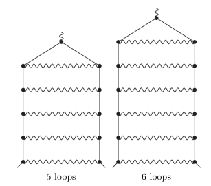
Figure 1: 5-loop and 6-loop ladder graphs

B Interval arithmetic

The interval arithmetic is an easy and reliable way for controlling round-off errors. In this way all calculations are performed with intervals, not with numbers. Arithmetic operations on intervals are defined in such a way that each exact intermediate value $x$ is quaranteed to be in the corresponding interval $[x^{-};x^{+}]$. One can use the following definitions:

$$[x^{-};x^{+}]+[y^{-};y^{+}]=[(x^{-}+y^{-})^{\text{down}};(x^{+}+y^{+})^{\text{up}}],$$

$$[x^{-};x^{+}]-[y^{-};y^{+}]=[(x^{-}-y^{+})^{\text{down}};(x^{+}-y^{-})^{\text{up}}],$$

$$[x^{-};x^{+}]\cdot[y^{-};y^{+}]=[\min((x^{-}y^{-})^{\text{down}},(x^{-}y^{+})^{\text{down}},(x^{+}y^{-})^{\text{down}},(x^{+}y^{+})^{\text{down}});$$

$$\max((x^{-}y^{-})^{\text{up}},(x^{-}y^{+})^{\text{up}},(x^{+}y^{-})^{\text{up}},(x^{+}y^{+})^{\text{up}})],$$

$$1/[x^{-};x^{+}]=[\min((1/x^{-})^{\text{down}},(1/x^{+})^{\text{down}});\max((1/x^{-})^{\text{up}},(1/x^{+})^{\text{up}})],$$

where $(*)^{\text{up}}$ and $(*)^{\text{down}}$ means the operation $(*)$ with rounding up (to $+\infty$) or down (to $-\infty$). The most of modern GPUs support specifying rounding mode for arithmetic operations and working with infinities for handling overflows. Addition, subtraction and multiplication can be realized directly by using the formulas proposed above. However, for division it is required to perform additional operations for handling divisions by zero and overflows. This does not slow down the computation because the amount of divisions in the integrand constructions is very small.

C Elimination of an interval arithmetic

The direct interval arithmetic is a very slow thing. However, there are many ways of increasing speed by weakening the distinctness of the intervals.

We will use the following specificity of the integrands construction. It is known  [30] how to construct the integrand for a given graph $G$ from the building blocks $V^{G^{\prime}}$, $Q^{G^{\prime}}_{a,j}$, $B^{G^{\prime}}_{ab}$, $S^{G^{\prime}}$, where $G^{\prime}$ is a graph that can be obtained from a subgraph of $G$ by shrinking some subgraphs to points, $a,b$ are internal electron lines of $G^{\prime}$, $j=1,2$, $V^{G^{\prime}}$ is defined through a sum over 1-trees of $G^{\prime}$, $Q^{G^{\prime}}_{a,j}$ through a sum over 1-trees passing $a$, $B^{G^{\prime}}_{ab}$ through a sum over trees with cycle passing $a,b$, $S^{G^{\prime}}$ through a sum over 2-trees. See the full definitions in  [30]. The construction rules described in  [30] give us to observe that for a high number of independent loops in $G$ the most part of the integrand computation is the calculations of polynomials with the variables $Q^{G^{\prime}}_{a,j}/V^{G^{\prime}}$ and $B^{G^{\prime}}_{ab}/V^{G^{\prime}}$.

Suppose we want to calculate a polynomial of the intervals $[x_{1}^{-};x_{1}^{+}],\ldots,[x_{n}^{-};x_{n}^{+}]$ that is constructed as a sequence of additions, subtractions and multiplications. The main ideas of the interval arithmetic elimination are:

• we can calculate the center of the resulting interval in the direct double-precision arithmetic using the same polynomial applied to the centers of $[x_{j}^{-};x_{j}^{+}]$;

• the radius of the resulting interval can be estimated as a function of $x_{j}^{-}$, $x_{j}^{+}$ that is much more simple than the source polynomial.

We will use the following inequality about the machine double-precision arithmetic:

$$|x-x^{\text{rnd}}|\leq 2^{-52}|x|+2^{-1022},$$

where $x^{\text{rnd}}$ corresponds to the machine representation of $x$ rounded in any direction.

Let $x_{j}$ be the exact values corresponding to the intervals $[x_{j}^{-};x_{j}^{+}]$, $j=1,\ldots,n$. By $x_{n+1},\ldots,x_{l}$ we denote the exact intermediate values that are obtained sequentially when we calculate the value of the needed polynomial. To each $j=1,\ldots,n$ we assign a type $t_{j}$: $t_{j}=0$ if $x_{j}$ is $Q^{G^{\prime}}_{a,k}/V^{G^{\prime}}$, $t_{j}=1$ if $x_{j}$ is $B^{G^{\prime}}_{ab}/V^{G^{\prime}}$ (we divide all source values into two groups in such a way because $|Q^{G^{\prime}}_{a,k}/V^{G^{\prime}}|\leq 1$, but $B^{G^{\prime}}_{ab}/V^{G^{\prime}}$ are unbounded). Let us define the numbers $x_{j}^{\text{appr}}$, $M_{j}$, $\varepsilon_{j}$, $j=1,\ldots,l$, satisfying the following conditions for all $j$:

• $|x_{j}^{\text{appr}}-x_{j}|\leq\varepsilon_{j}$;

• $|x_{j}^{\text{appr}}|\leq M_{j}$.

We define them by using the following rules:

• $x_{j}^{\text{appr}}=((x_{j}^{-}+x_{j}^{+})/2)^{\text{rnd}}$, $j=1,\ldots,n$ (thus, $x_{j}^{\text{appr}}$ are the centers of the corresponding intervals; the machine double-precision arithmetic guarantees that we always have $x_{j}^{-}\leq x_{j}^{\text{appr}}\leq x_{j}^{+}$ if an overflow does not occur);

• $M_{j}$ are defined for $j=1,\ldots,n$ by

  $$M_{j}=\max_{t_{k}=t_{j}}|x_{k}^{\text{appr}}|;$$

• $\varepsilon_{j}$ are defined for $j=1,\ldots,n$ by

  $$\varepsilon_{j}=\varepsilon=\max_{1\leq k\leq n}\max\left((x_{k}^{\text{appr}}-x_{k}^{+})^{\text{up}},(x_{k}^{+}-x_{k}^{\text{appr}})^{\text{up}}\right),$$

• if $x_{j}$ is obtained as $x_{k}*x_{r}$, where $*$ is the addition, subtraction or multiplication, $j=n+1,\ldots,l$, then $x_{j}^{\text{appr}}=(x_{k}^{\text{appr}}*x_{r}^{\text{appr}})^{\text{rnd}}$ (thus, $x_{j}^{\text{appr}}$ are obtained by the direct double-precision arithmetic without specifying the rounding mode);

• analogously, $(M_{j},\varepsilon_{j})$ is defined by

  $$(M_{j},\varepsilon_{j})=((M_{k}+M_{r})(1+2^{-52})+2^{-1022},\varepsilon_{k}+\varepsilon_{r}+2^{-52}(M_{k}+M_{r})+2^{-1022})$$

  for addition and subtraction, and by

  $$(M_{j},\varepsilon_{j})=(M_{k}M_{r}(1+2^{-52})+2^{-1022},$$

  $$\varepsilon_{k}\varepsilon_{r}+\varepsilon_{k}M_{r}+\varepsilon_{r}M_{k}+2^{-52}M_{k}M_{r}+2^{-1022})$$

  for multiplication.

It is easy to see that for the final $l$ the value $\varepsilon_{l}$ can be expressed as a polynomial $P(M_{t=0},M_{t=1},\varepsilon)$ with positive coefficients in only three variables, where

$$M_{t=a}=\max_{t_{k}=a}|x_{k}^{\text{appr}}|.$$

Thus, the value of $\varepsilon_{l}$ can be obtained directly using the coefficients of this polynomial without calculating the intermediate values $M_{k},\varepsilon_{k}$.

However, the polynomial

$$P(M_{t=0},M_{t=1},\varepsilon)=\sum_{u,v,w}C_{u,v,w}(M_{t=0})^{u}(M_{t=1})^{v}\varepsilon^{w}$$

can still have many coefficients and therefore can require a lot of arithmetic operations for computation. We estimate $P$ by another expression in the following way. Let us split $P$ into four parts $P_{0}$, $P_{1}$, $P_{2}$, $P_{3}$ by the following rules:

$$P_{0}:\ C_{u,v,w}<2^{-100},\quad P_{1}:\ 2^{-100}\leq C_{u,v,w}<0.5,$$

$$P_{2}:\ C_{u,v,w}\geq 0.5,\ w\leq 1,\quad P_{3}:\ C_{u,v,w}\geq 0.5,\ w\geq 2.$$

Thus, $P=P_{0}+P_{1}+P_{2}+P_{3}$. By definition, put

$$u_{j}^{-}=\min_{C_{u,v,w}^{j}>0}u,\quad u_{j}^{+}=\max_{C_{u,v,w}^{j}>0}u,$$

where

$$P_{j}(M_{t=0},M_{t=1},\varepsilon)=\sum_{u,v,w}C_{u,v,w}^{j}(M_{t=0})^{u}(M_{t=1})^{v}\varepsilon^{w},\quad j=0,1,2,3.$$

Let us define $v_{j}^{-}$, $v_{j}^{+}$, $w_{j}^{-}$, $w_{j}^{+}$ in analogous way. Put

$$P_{j}^{\prime}(M_{t=0},M_{t=1},\varepsilon)=\left(\sum_{u,v,w}C_{u,v,w}^{j}\right)$$

$$\cdot\max\left((M_{t=0})^{u_{j}^{+}},(M_{t=0})^{u_{j}^{-}}\right)\cdot\max\left((M_{t=1})^{v_{j}^{+}},(M_{t=1})^{v_{j}^{-}}\right)\cdot\max\left(\varepsilon^{w_{j}^{+}},\varepsilon^{w_{j}^{-}}\right).$$

It is obvious that $P_{j}^{\prime}\geq P_{j}$. So, we can use $P^{\prime}=P_{0}^{\prime}+P_{1}^{\prime}+P_{2}^{\prime}+P_{3}^{\prime}$ as a radius of the final interval, if it is calculated by machine arithmetic operations with rounding up. $P^{\prime}$ is much simpler for calculation than $P$. Thus, an interval for the final value may be

$$[(x_{l}^{\text{appr}}-(P^{\prime})^{\text{up}})^{\text{down}};(x_{l}^{\text{appr}}+(P^{\prime})^{\text{up}})^{\text{up}}].$$

We split $P$ into four polynomials in such a way guiding the following considerations:

• $P_{3}$ contains the most of the coefficients sum; however, its contribution in $P_{3}^{\prime}$ will be compensated by the multiplier $\varepsilon^{2}$ (when $\varepsilon$ is near zero);

• $P_{2}$ has a big sum of coefficients too; however, it is much less than $P_{3}$ has; this sum will be compensated by the multiplier $\varepsilon$ in $P_{2}^{\prime}$;

• $P_{1}$ has a little sum of coefficients; however, in some cases $P_{1}^{\prime}$ can be noticeable; thus, we separate $P_{1}$ from $P_{0}$ to minimize the contribution of the $\max\cdot\max\cdot\max$ part in the definition of $P_{1}^{\prime}$;

• the contribution of the coefficients of $P_{0}$ is always small.

D Algorithm of obtaining accurate integrand values

We obtain the value $I(\underline{z})/g(\underline{z})$ from (12) first by the eliminated interval arithmetic from Section IV.C. If the obtained interval $[y^{-};y^{+}]$ does not satisfy the condition $y^{+}-y^{-}\leq\sigma/4$, where $\sigma$ is the current error estimation for the obtained integral value, we repeat the calculation in the direct double-precision interval arithmetic. If it is not enough, we reiterate this calculation in the interval arithmetic based on floating-point numbers with 128-bit mantissa and with 256-bit mantissa (if needed). If the 256-bit mantissa precision is not enough, we suppose that the value equals $0$.

The arithmetic with 128-bit mantissa is realized on GPU in such a way that all operations are performed with the GPU register memory. The arithmetic with 256-bit mantissa works with the global GPU memory. The usage of the register memory improves the performance by about 10 times.

We also use a routine for prevention of emerging occasional very large values that is analogous to the one described in  [29], but adapted for GPU parallel computing.

E Modified probability density functions

It is theoretically possible the situation when $g(\underline{z})$ from (12) is very small, but the smallness of $|I(\underline{z})|$ does not correspond to it. An emergence of such situations can make the Monte Carlo convergence worse. For patching it we use the probability density functions

$$g(\underline{z})=C_{1}g_{1}(\underline{z})+C_{2}g_{2}(\underline{z})+C_{3}g_{3}(\underline{z})+C_{4}g_{4}(\underline{z})$$

instead of (13), (14), where $g_{1}$ is defined by (13), (14),

$$g_{2}(z_{1},\ldots,z_{n})=\frac{\prod_{l=2}^{n}\left[\mathrm{Deg}(\{j_{l},j_{l+1},\ldots,j_{n}\})(z_{j_{l}}/z_{j_{l-1}})^{\mathrm{Deg}(\{j_{l},j_{l+1},\ldots,j_{n}\})}\right]}{n!z_{1}z_{2}\ldots z_{n}},$$

when the definitions from Section III are used, $g_{3}$ is defined by (13), (14), but with same $\mathrm{Deg}(s)=D$, $g_{4}(\underline{z})=(n-1)!$ (the uniform distribution). To generate a random sample with the distribution $g(\underline{z})$ we should perform the following two steps:

• generate randomly $j=1,2,3,4$, where the probability of selecting $j$ is $C_{j}$;

• generate a sample with the distribution $g_{j}(\underline{z})$.

The generation with the distribition $g_{2}(\underline{z})$ is the same as for distributions defined by (13), (14), but at the stage of sector generation we must take sectors with same probabilities, see  [29]. All computations are performed with the following values for the constants:

$$D=0.75,\ C_{2}=0.03,\ C_{3}=0.035,\ C_{4}=0.035,\ C_{1}=1-C_{2}-C_{3}-C_{4}.$$

F Monte Carlo error estimation

Let $\underline{z}_{1},\ldots,\underline{z}_{N}$ be random samples, the formula (12) is used for Monte Carlo integration. By definition, put $y_{j}=I(\underline{z})/g(\underline{z})$. The conventional error estimation approach is based on the following formula for the standard deviation:

$$(\sigma_{\downarrow})^{2}=\frac{\sum_{j=1}^{N}y_{j}^{2}}{N^{2}}-\frac{\left(\sum_{j=1}^{N}y_{j}\right)^{2}}{N^{3}}.$$

However, this formula has a tendency to underestimate the real standard deviation. Let us consider the 5-loop and 6-loop ladder examples. By definition, put

$$\mathrm{maxlog}=\max_{j}\lfloor\log_{2}|y_{j}|+0.5\rfloor,$$

let $n_{k}$ be the quantity of samples $j$ such that

$$2^{\mathrm{maxlog}-k-0.5}\leq|y_{j}|<2^{\mathrm{maxlog}-k+0.5}.$$ (16)

$\mathrm{maxlog}$ and $n_{j}$ for the 5-loop and 6-loop ladders are presented in Table LABEL:table_distr_ladder. $n_{k}$ is an approximation for $Np_{k}$, where $p_{k}$ is the probability that a sample is in the interval (16). We can see that the real standard deviation is highly dependent on the behavior of $p_{j}$ for $j<0$. For example, if $p_{j+1}/p_{j}<4$ for all $j<j_{0}$ then the standard deviation is infinite.

We will use the improved estimation

$$(\sigma_{\uparrow})^{2}=(\sigma_{\downarrow})^{2}+\triangle_{\text{uncert}}+\triangle_{\text{peak}},$$

where

$$\triangle_{\text{uncert}}=4\cdot\max_{k=0}^{19}4^{\mathrm{maxlog}-k}\sqrt{n_{k}}$$

is the contribution of the uncertainty of $n_{k}$, $\triangle_{\text{peak}}$ is the contribution of the predicted behavior of $p_{j}$ for $j<0$ that is described below.

The idea is to approximate $n_{j}$ by a geometric progression taking into account that $n_{j}$ are known with an uncertainty of about $C\sqrt{n_{j}}$ and that $p_{j+1}/p_{j}$ changes with $j$.

Put

$$h_{j}=\begin{cases}\log_{2}n_{j},\text{ if }n_{j}>0,\\ -2,\text{ if }n_{j}=0,\end{cases}$$

$$h_{j}^{\pm}=\log_{2}\max\left(\frac{1}{8},n_{j}+\frac{1}{2}\pm\sqrt{n_{j}+\frac{1}{4}}\right),$$

Here $h_{j}$ is an approximated value of $\log_{2}(Np_{j})$, $[h_{j}^{-};h_{j}^{+}]$ is an interval for this value that is obtained taking into account that $n_{j}$ is known with uncertainty.

We will estimate the absolute value of a difference between neighbour $\log_{2}(p_{j+1}/p_{j})$ by the value $d$, where

$$d=\max_{0\leq j<k\leq 18}\frac{d_{jk}}{k-j},$$

where $d_{jk}$ is the distance from $0$ to the interval $[d_{jk}^{-};d_{jk}^{+}]$,

$$d_{jk}^{-}=(h_{k+1}^{-}-h_{k}^{+})-(h_{j+1}^{+}-h_{j}^{-}),\quad d_{jk}^{+}=(h_{k+1}^{+}-h_{k}^{-})-(h_{j+1}^{-}-h_{j}^{+}).$$

For approximation of the sequence by a progression we will use another values for $\log_{2}(Np_{j})$ uncertainty that are obtained taking into account that errors for lesser $j$ are more critical:

$$u_{j}=\begin{cases}\frac{1}{2}\left[\log_{2}\left(n_{j}+\frac{C_{j}^{2}}{2}+C_{j}\sqrt{n_{j}+\frac{C_{j}^{2}}{4}}\right)-\log_{2}\left(n_{j}+\frac{C_{j}^{2}}{2}-C_{j}\sqrt{n_{j}+\frac{C_{j}^{2}}{4}}\right)\right],\\ \quad\text{ if }n_{j}>0,\\ 3,\text{ if }n_{j}=0,\end{cases}$$

where

$$C_{j}=\frac{2}{1+\frac{2(j+1)}{20}}.$$

For approximating the sequence of logarithms by a linear function $kj+b$ let us introduce coefficients $a^{l}_{j}$, $f^{l}_{j}$, $2\leq l\leq 20$, $0\leq j<l$, for the least squares method:

$$\left(\sum_{j=0}^{l-1}a^{l}_{j}x_{j};\sum_{j=0}^{l-1}f^{l}_{j}x_{j}\right)=\mathrm{argmin}_{(k;b)}\sum_{j=0}^{l-1}(kj+b-x_{j})^{2}$$

for all $l$ and $x_{0},\ldots,x_{l-1}$.

Put

$$k_{l}=\sum_{j=0}^{l-1}a^{l}_{j}h_{j}-\sqrt{\sum_{j=0}^{l-1}(a^{l}_{j})^{2}u_{j}^{2}}-d\sum_{j=0}^{l-1}\frac{j(j-1)a^{l}_{j}}{2},$$

$$k=\max(k_{2},\ldots,k_{20},h_{0}-1-u_{0}).$$

This formula takes into account both uncertainty of $n_{j}$ and shift of $p_{j+1}/p_{j}$ with $j$. We take $\max$ to prevent from excessive overestimation. Also, put

$$\triangle b=\min_{l}\left(\sqrt{\sum_{j=0}^{l-1}(f^{l}_{j})^{2}u_{j}^{2}}+d\sum_{j=0}^{l-1}\frac{j(j-1)f^{l}_{j}}{2}\right),$$

$b=\sum_{j=0}^{l-1}f^{l}_{j}h_{j}$, where we take $l$ for which the minimum is achieved. Let us define $\triangle_{\text{peak}}$ by

$$\triangle_{\text{peak}}=2^{2\cdot\mathrm{maxlog}+b+0.7\triangle b}\left(\frac{1}{1-2^{-w}}-1\right),$$

where

$$w=\frac{k-\frac{17}{8}+\sqrt{\left(k-\frac{17}{8}\right)^{2}+\frac{1}{16}}}{2}+\frac{1}{8}.$$

The meaning of this definition is that we use the formula for the sum of a geometric progression taking $w$ instead of $k-2$. $w$ is defined in such a way that $w\sim k-2$ as $k\rightarrow+\infty$ and $w\rightarrow 1/8$ as $k\rightarrow-\infty$.

We use $\sigma_{\uparrow}$ for all numerical results that are presented in this paper.

Tables LABEL:table_dependence_4loops, LABEL:table_dependence_5loops, LABEL:table_dependence_6loops contain the dependence of the error estimations and the real errors on numbers of samples $N_{\text{total}}$ for $A_{1}^{(8)}[\text{no lepton loops}]$, 5-loop and 6-loop ladders respectively.

Table I: Probability distributions for 5-loop ladder and 6-loop ladder

Parameter	5-loop ladder	6-loop ladder
maxlog	$23$	$28$
$n_{0}$	$11$	$2$
$n_{1}$	$64$	$8$
$n_{2}$	$393$	$45$
$n_{3}$	$2300$	$174$
$n_{4}$	$11891$	$785$
$n_{5}$	$51840$	$2898$
$n_{6}$	$204817$	$9374$
$n_{7}$	$688060$	$25759$
$n_{8}$	$1885211$	$62363$
$n_{9}$	$4300121$	$135343$
$n_{10}$	$8615210$	$267630$
$n_{11}$	$15701395$	$490720$
$n_{12}$	$26582404$	$849862$
$n_{13}$	$42456874$	$1394740$
$n_{14}$	$64590501$	$2198221$
$n_{15}$	$94011212$	$3331999$
$n_{16}$	$131314678$	$4892615$
$n_{17}$	$176228467$	$6965326$
$n_{18}$	$228021742$	$9626392$
$n_{19}$	$285614048$	$12965533$

Table II: Dependence of the estimated error and the difference between the obtained value and the known semianalytical one  [8] on the number of Monte Carlo samples $N_{\text{total}}$: $A_{1}^{(8)}[\text{no lepton loops}]$, see a remark about $\sigma_{\uparrow}$, $\sigma_{\downarrow}$ calculation in Section IV.H

$N_{\text{total}}$	Value	$\sigma_{\uparrow}$	$\sigma_{\downarrow}$	Difference	$\sigma_{\uparrow}/\sigma_{\downarrow}$
$40\times 10^{9}$	$-2.3937$	$0.2144$	$0.1168$	$-0.2168$	$1.84$
$10^{11}$	$-2.2323$	$0.0710$	$0.0494$	$-0.0555$	$1.44$
$20\times 10^{10}$	$-2.1820$	$0.0468$	$0.0345$	$-0.0051$	$1.36$
$50\times 10^{10}$	$-2.1851$	$0.0282$	$0.0218$	$-0.0083$	$1.30$
$10^{12}$	$-2.1757$	$0.0194$	$0.0154$	$0.0012$	$1.26$
$20\times 10^{11}$	$-2.1702$	$0.0133$	$0.0109$	$0.0066$	$1.23$
$32\times 10^{11}$	$-2.1807$	$0.0104$	$0.0086$	$-0.0038$	$1.21$

Table III: Dependence of the estimated error and the difference between the obtained value and the known analytical one  [49] on the number of Monte Carlo samples $N_{\text{total}}$: 5-loop ladder

$N_{\text{total}}$	Value	$\sigma_{\uparrow}$	$\sigma_{\downarrow}$	Difference	$\sigma_{\uparrow}/\sigma_{\downarrow}$
$59\times 10^{5}$	$12.0682$	$0.8202$	$0.3288$	$0.4090$	$2.49$
$12\times 10^{7}$	$11.6120$	$0.1349$	$0.0720$	$-0.0472$	$1.87$
$24\times 10^{7}$	$11.6934$	$0.0800$	$0.0525$	$0.0342$	$1.52$
$60\times 10^{7}$	$11.6798$	$0.0665$	$0.0379$	$0.0206$	$1.76$
$10^{9}$	$11.6678$	$0.0427$	$0.0270$	$0.0086$	$1.58$
$20\times 10^{8}$	$11.6474$	$0.0277$	$0.0192$	$-0.0118$	$1.44$
$50\times 10^{8}$	$11.6448$	$0.0150$	$0.0120$	$-0.0144$	$1.25$
$10^{10}$	$11.6509$	$0.0111$	$0.0086$	$-0.0083$	$1.29$
$20\times 10^{9}$	$11.6541$	$0.0073$	$0.0061$	$-0.0051$	$1.19$
$29\times 10^{9}$	$11.6530$	$0.0058$	$0.0050$	$-0.0062$	$1.16$

Table IV: Dependence of the estimated error and the difference between the obtained value and the known analytical one  [49] on the number of Monte Carlo samples $N_{\text{total}}$: 6-loop ladder

$N_{\text{total}}$	Value	$\sigma_{\uparrow}$	$\sigma_{\downarrow}$	Difference	$\sigma_{\uparrow}/\sigma_{\downarrow}$
$15\times 10^{6}$	$34.3209$	$7.1538$	$2.0690$	$-0.0461$	$3.46$
$65\times 10^{7}$	$35.4566$	$1.1201$	$0.4659$	$1.0896$	$2.40$
$97\times 10^{7}$	$35.0500$	$0.7556$	$0.3566$	$0.6829$	$2.12$
$12\times 10^{8}$	$35.0187$	$0.6808$	$0.3201$	$0.6517$	$2.13$
$22\times 10^{8}$	$34.5855$	$0.4217$	$0.2276$	$0.2185$	$1.85$
$41\times 10^{8}$	$34.3967$	$0.3020$	$0.1675$	$0.0297$	$1.80$
$70\times 10^{8}$	$34.3651$	$0.2320$	$0.1337$	$-0.0019$	$1.74$
$10^{10}$	$34.3062$	$0.1974$	$0.1137$	$-0.0608$	$1.74$

G Contributions of individual Feynman graphs

The contributions of 2-loop and 3-loop Feynman graphs to $A_{1}^{(4)}$ and $A_{1}^{(6)}$ are presented in Tables LABEL:table_indi_2loops and LABEL:table_indi_3loops. The corresponding pictures are FIG. 3 and FIG. 4. Each individual contribution in this paper is given for a Feynman graph without arrow directions on electron lines and includes the contributions of the corresponding graphs with all directions (that are the same). The 4-loop graphs are split into gauge invariant classes $(k,m,m^{\prime})$, where $m$ and $m^{\prime}$ are numbers of internal photon lines to the left and to the right from the external photon line (or vice versa), $k$ is the number of photons with the ends on the opposite sides of it. We do not give a picture for 4-loop graphs, but they are encoded in the tables as expressions of the form

$$p;\ s_{1}-f_{1},\ s_{2}-f-2,\ s_{3}-f_{3},\ s_{4}-f_{4},$$

where $p$ is the number of vertex that is incident to the external photon line, $s_{j}$ and $f_{j}$ are the ends of the $j$-th internal photon line, the vertexes are enumerated from $1$ to $9$ along the electron path, $s_{j}<f_{j}$, $s_{1}<\ldots<s_{4}$. The graphs are ordered lexicographically, and we guarantee that the code of a graph is the lexicographically minimal one. For example, the code of the graph from FIG. 2 is

$$3;\ 1-8,\ 2-7,\ 4-5,\ 6-9.$$

Figure 2: 4-loop Feynman graph: example

The contributions of the 4-loop graphs are presented in Tables LABEL:table_indi_4loops_1_3_0, LABEL:table_indi_4loops_2_2_0, LABEL:table_indi_4loops_1_2_1, LABEL:table_indi_4loops_3_1_0, LABEL:table_indi_4loops_2_1_1, LABEL:table_indi_4loops_4_0_0. The numbers of the graphs for which the contribution must coincide with the contribution obtained by the direct subtraction on the mass shell in Feynman gauge are marked by a star ^∗, see Section IV.H.

The fields of the tables have the following meaning:

• Value is the obtained value for the contribution with the uncertainty $\sigma_{\uparrow}$, see Section IV.F;

• $\sigma_{\uparrow}/\sigma_{\downarrow}$ is the relation between the improved standard deviation and the conventional one, see Section IV.F;

• $N_{\text{total}}$ is the total quantity of Monte Carlo samples;

• $N^{\text{fail}}_{\text{EIA}}$ is the quantity of samples for which the Eliminated Interval Arithmetic from Section IV.C failed;

• $\triangle^{\text{fail}}_{\text{EIA}}$ is the contribution of that samples;

• $N^{\text{fail}}_{\text{IA}}$ is the quantity of samples for which the direct double-precision interval arithmetic from Section IV.B failed;

• $\triangle^{\text{fail}}_{\text{IA}}$ is the contribution of that samples;

• $N^{\text{fail}}_{\text{128}}$ is the quantity of samples for which the interval arithmetic based on numbers with 128-bit mantissa failed;

• $\triangle^{\text{fail}}_{\text{128}}$ is the contribution of that samples.

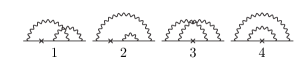
Figure 3: 2-loop Feynman graphs without lepton loops

Table V: Contributions of individual Feynman graphs from FIG. 3 to $A^{(4)}_{1}$

Number	Graph	Value	$N_{\text{total}}$	$N_{\text{EIA}}^{\text{fail}}$	$N_{\text{IA}}^{\text{fail}}$	$N_{\text{128}}^{\text{fail}}$	$\triangle_{\text{EIA}}^{\text{fail}}$	$\triangle_{\text{IA}}^{\text{fail}}$	$\triangle_{\text{128}}^{\text{fail}}$	$\sigma_{\uparrow}/\sigma_{\downarrow}$
$1$	2; 1-4, 3-5	-0.0640193(19)	$94\times 10^{10}$	$26\times 10^{8}$	$32\times 10^{4}$	$0$	$0.003$	$2\times 10^{-6}$	$0$	1.04
$2$	2; 1-5, 3-4	-0.5899758(14)	$58\times 10^{10}$	$61\times 10^{7}$	$50\times 10^{6}$	$2$	$-0.0005$	$-2\times 10^{-6}$	$-2\times 10^{-19}$	1.00
$3$	3; 1-4, 2-5	-0.4676475(17)	$90\times 10^{10}$	$44\times 10^{7}$	$57479$	$0$	$-0.008$	$-10^{-5}$	$0$	1.05
$4$	3; 1-5, 2-4	0.7774774(18)	$92\times 10^{10}$	$34\times 10^{8}$	$17\times 10^{6}$	$0$	$0.007$	$0.0002$	$0$	1.00

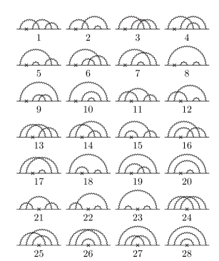
Figure 4: 3-loop Feynman graphs without lepton loops

Table VI: Contributions of individual Feynman graphs from FIG. 4 to $A^{(6)}_{1}$

Number	Graph	Value	$N_{\text{total}}$	$N_{\text{EIA}}^{\text{fail}}$	$N_{\text{IA}}^{\text{fail}}$	$N_{\text{128}}^{\text{fail}}$	$\triangle_{\text{EIA}}^{\text{fail}}$	$\triangle_{\text{IA}}^{\text{fail}}$	$\triangle_{\text{128}}^{\text{fail}}$	$\sigma_{\uparrow}/\sigma_{\downarrow}$
$1$	2; 1-4, 3-6, 5-7	-1.679616(20)	$29\times 10^{10}$	$57\times 10^{8}$	$33\times 10^{4}$	$0$	$-0.1$	$-5\times 10^{-5}$	$0$	1.08
$2$	2; 1-4, 3-7, 5-6	0.832792(20)	$28\times 10^{10}$	$40\times 10^{8}$	$26\times 10^{6}$	$0$	$0.1$	$0.0009$	$0$	1.10
$3$	2; 1-5, 3-6, 4-7	0.214875(14)	$19\times 10^{10}$	$22\times 10^{8}$	$88\times 10^{4}$	$1$	$0.01$	$7\times 10^{-5}$	$-4\times 10^{-24}$	1.05
$4$	2; 1-5, 3-7, 4-6	-0.028928(11)	$11\times 10^{10}$	$30\times 10^{8}$	$10^{6}$	$2$	$-0.004$	$-3\times 10^{-5}$	$-10^{-11}$	1.03
$5$	2; 1-6, 3-4, 5-7	-0.097163(26)	$47\times 10^{10}$	$16\times 10^{9}$	$13\times 10^{7}$	$10$	$-0.002$	$10^{-5}$	$3\times 10^{-16}$	1.16
$6$	2; 1-6, 3-5, 4-7	0.144471(12)	$14\times 10^{10}$	$31\times 10^{8}$	$23\times 10^{4}$	$3$	$0.06$	$9\times 10^{-6}$	$-2\times 10^{-36}$	1.02
$7$	2; 1-6, 3-7, 4-5	0.804106(17)	$22\times 10^{10}$	$26\times 10^{8}$	$18\times 10^{6}$	$1$	$0.02$	$-0.0001$	$-10^{-61}$	1.08
$8$	2; 1-7, 3-4, 5-6	-2.123267(16)	$17\times 10^{10}$	$34\times 10^{8}$	$48\times 10^{7}$	$4496$	$-0.02$	$-0.0002$	$-10^{-12}$	1.00
$9$	2; 1-7, 3-5, 4-6	2.524749(18)	$19\times 10^{10}$	$89\times 10^{8}$	$18\times 10^{6}$	$0$	$0.07$	$2\times 10^{-5}$	$0$	1.00
$10$	2; 1-7, 3-6, 4-5	-0.058729(11)	$11\times 10^{10}$	$51\times 10^{8}$	$53\times 10^{6}$	$6$	$0.009$	$-2\times 10^{-5}$	$-10^{-15}$	1.00
$11$	3; 1-4, 2-6, 5-7	5.042278(27)	$57\times 10^{10}$	$91\times 10^{8}$	$38\times 10^{5}$	$5$	$0.5$	$0.0004$	$8\times 10^{-23}$	1.09
$12$	3; 1-4, 2-7, 5-6	-3.500634(25)	$50\times 10^{10}$	$65\times 10^{8}$	$52\times 10^{6}$	$2$	$-0.4$	$-0.02$	$-3\times 10^{-22}$	1.06
$13$	3; 1-5, 2-6, 4-7	-1.757945(15)	$27\times 10^{10}$	$97\times 10^{7}$	$34\times 10^{5}$	$10$	$-0.05$	$-0.0002$	$8\times 10^{-13}$	1.10
$14$	3; 1-5, 2-7, 4-6	0.140129(14)	$18\times 10^{10}$	$35\times 10^{8}$	$40\times 10^{5}$	$10$	$0.003$	$9\times 10^{-7}$	$5\times 10^{-21}$	1.06
$15$	3; 1-6, 2-4, 5-7	-3.257290(27)	$48\times 10^{10}$	$16\times 10^{9}$	$28\times 10^{6}$	$5$	$-0.3$	$-0.004$	$-10^{-8}$	1.00
$16$	3; 1-6, 2-5, 4-7	-0.334691(14)	$23\times 10^{10}$	$13\times 10^{8}$	$30\times 10^{5}$	$7$	$-0.07$	$-0.0005$	$10^{-12}$	1.13
$17$	3; 1-6, 2-7, 4-5	0.315388(22)	$43\times 10^{10}$	$20\times 10^{8}$	$16\times 10^{6}$	$0$	$-0.003$	$-5\times 10^{-8}$	$0$	1.03
$18$	3; 1-7, 2-4, 5-6	4.513076(27)	$43\times 10^{10}$	$22\times 10^{9}$	$46\times 10^{7}$	$2909$	$0.4$	$0.04$	$2\times 10^{-6}$	1.00
$19$	3; 1-7, 2-5, 4-6	0.611112(21)	$28\times 10^{10}$	$67\times 10^{8}$	$37\times 10^{5}$	$1$	$0.1$	$0.0006$	$-10^{-24}$	1.15
$20$	3; 1-7, 2-6, 4-5	-2.269647(16)	$19\times 10^{10}$	$27\times 10^{8}$	$39\times 10^{6}$	$0$	$-0.09$	$-0.001$	$0$	1.00
$21$	4; 1-3, 2-6, 5-7	-2.908437(22)	$34\times 10^{10}$	$81\times 10^{8}$	$50\times 10^{4}$	$0$	$-0.4$	$-0.0005$	$0$	1.01
$22$	4; 1-3, 2-7, 5-6	6.533883(31)	$60\times 10^{10}$	$20\times 10^{9}$	$16\times 10^{7}$	$9$	$0.9$	$0.03$	$2\times 10^{-8}$	1.01
$23$	4; 1-7, 2-3, 5-6	-3.204367(20)	$24\times 10^{10}$	$35\times 10^{8}$	$56\times 10^{7}$	$5040$	$-0.2$	$-0.05$	$-3\times 10^{-6}$	1.00
$24$	4; 1-5, 2-6, 3-7	-0.0267956(78)	$10^{11}$	$37\times 10^{7}$	$35\times 10^{5}$	$5$	$-0.02$	$-0.0007$	$-6\times 10^{-12}$	1.07
$25$	4; 1-5, 2-7, 3-6	1.861914(17)	$31\times 10^{10}$	$19\times 10^{8}$	$14\times 10^{6}$	$43$	$0.1$	$-0.0004$	$-2\times 10^{-12}$	1.08
$26$	4; 1-6, 2-7, 3-5	-0.945906(11)	$14\times 10^{10}$	$36\times 10^{8}$	$13\times 10^{5}$	$0$	$-0.07$	$-0.0005$	$0$	1.01
$27$	4; 1-7, 2-5, 3-6	-2.230794(19)	$31\times 10^{10}$	$36\times 10^{8}$	$11\times 10^{6}$	$24$	$-0.2$	$-0.0009$	$-5\times 10^{-21}$	1.10
$28$	4; 1-7, 2-6, 3-5	1.790285(19)	$28\times 10^{10}$	$83\times 10^{8}$	$22\times 10^{6}$	$1$	$0.1$	$0.003$	$-5\times 10^{-9}$	1.01

Table VII: Contributions of graphs from the gauge-invariant class $(1,3,0)$ to $A^{(8)}_{1}$

Number	Graph	Value	$N_{\text{total}}$	$N_{\text{EIA}}^{\text{fail}}$	$N_{\text{IA}}^{\text{fail}}$	$N_{\text{128}}^{\text{fail}}$	$\triangle_{\text{EIA}}^{\text{fail}}$	$\triangle_{\text{IA}}^{\text{fail}}$	$\triangle_{\text{128}}^{\text{fail}}$	$\sigma_{\uparrow}/\sigma_{\downarrow}$
$1$	2; 1-4, 3-6, 5-8, 7-9	2.19701(73)	$15\times 10^{9}$	$92\times 10^{7}$	$27780$	$0$	$0.6$	$0.0001$	$0$	1.56
$2$	2; 1-4, 3-6, 5-9, 7-8	-3.81327(91)	$23\times 10^{9}$	$95\times 10^{7}$	$11\times 10^{5}$	$1$	$-1$	$-0.01$	$2\times 10^{-45}$	1.65
$3$	2; 1-4, 3-7, 5-8, 6-9	0.55330(31)	$49\times 10^{8}$	$23\times 10^{7}$	$31677$	$1$	$0.2$	$0.0001$	$9\times 10^{-29}$	1.52
$4$	2; 1-4, 3-7, 5-9, 6-8	1.82177(56)	$10^{10}$	$57\times 10^{7}$	$47919$	$2$	$0.5$	$0.0002$	$10^{-36}$	1.51
$5$	2; 1-4, 3-8, 5-6, 7-9	-2.43257(93)	$23\times 10^{9}$	$13\times 10^{8}$	$29\times 10^{5}$	$1$	$-0.8$	$-0.008$	$10^{-35}$	1.72
$6$	2; 1-4, 3-8, 5-7, 6-9	0.95204(51)	$89\times 10^{8}$	$50\times 10^{7}$	$26741$	$1$	$0.3$	$8\times 10^{-5}$	$-4\times 10^{-55}$	1.41
$7$	2; 1-4, 3-8, 5-9, 6-7	-2.19745(69)	$15\times 10^{9}$	$57\times 10^{7}$	$54\times 10^{4}$	$0$	$-0.4$	$-0.003$	$0$	1.89
$8$	2; 1-4, 3-9, 5-6, 7-8	2.1481(10)	$20\times 10^{9}$	$75\times 10^{7}$	$27\times 10^{6}$	$161$	$0.8$	$0.03$	$-6\times 10^{-7}$	1.65
$9$	2; 1-4, 3-9, 5-7, 6-8	-2.48196(92)	$26\times 10^{9}$	$19\times 10^{8}$	$98\times 10^{4}$	$6$	$-0.7$	$-0.004$	$-9\times 10^{-40}$	1.54
$10$	2; 1-4, 3-9, 5-8, 6-7	0.98718(84)	$19\times 10^{9}$	$12\times 10^{8}$	$33\times 10^{5}$	$3$	$0.5$	$0.008$	$2\times 10^{-41}$	1.61
$11$	2; 1-5, 3-6, 4-8, 7-9	-1.38009(58)	$12\times 10^{9}$	$54\times 10^{7}$	$90636$	$4$	$-0.3$	$-0.0002$	$-2\times 10^{-31}$	1.63
$12$	2; 1-5, 3-6, 4-9, 7-8	1.16697(56)	$12\times 10^{9}$	$37\times 10^{7}$	$55\times 10^{4}$	$5$	$0.2$	$0.002$	$4\times 10^{-52}$	1.48
$13$	2; 1-5, 3-7, 4-8, 6-9	0.66741(35)	$58\times 10^{8}$	$15\times 10^{7}$	$31\times 10^{4}$	$22$	$-0.03$	$-0.001$	$-3\times 10^{-14}$	1.29
$14$	2; 1-5, 3-7, 4-9, 6-8	-0.26457(35)	$48\times 10^{8}$	$22\times 10^{7}$	$38\times 10^{4}$	$61$	$-0.06$	$-10^{-5}$	$5\times 10^{-11}$	1.25
$15$	2; 1-5, 3-8, 4-6, 7-9	1.05969(43)	$63\times 10^{8}$	$42\times 10^{7}$	$44335$	$3$	$0.2$	$7\times 10^{-5}$	$9\times 10^{-41}$	1.31
$16$	2; 1-5, 3-8, 4-7, 6-9	0.47610(29)	$49\times 10^{8}$	$15\times 10^{7}$	$39328$	$3$	$0.06$	$-0.0004$	$-5\times 10^{-30}$	1.51
$17$	2; 1-5, 3-8, 4-9, 6-7	0.47497(36)	$62\times 10^{8}$	$12\times 10^{7}$	$20\times 10^{4}$	$4$	$0.2$	$0.0003$	$6\times 10^{-36}$	1.21
$18$	2; 1-5, 3-9, 4-6, 7-8	-1.10746(43)	$63\times 10^{8}$	$40\times 10^{7}$	$90\times 10^{4}$	$1$	$-0.1$	$-0.0004$	$7\times 10^{-35}$	1.35
$19$	2; 1-5, 3-9, 4-7, 6-8	-0.23411(34)	$47\times 10^{8}$	$26\times 10^{7}$	$33298$	$2$	$-0.09$	$5\times 10^{-5}$	$-3\times 10^{-35}$	1.53
$20$	2; 1-5, 3-9, 4-8, 6-7	0.13458(26)	$37\times 10^{8}$	$12\times 10^{7}$	$16\times 10^{4}$	$0$	$0.03$	$0.0001$	$0$	1.08
$21$	2; 1-6, 3-4, 5-8, 7-9	1.35348(94)	$23\times 10^{9}$	$17\times 10^{8}$	$57\times 10^{5}$	$2$	$0.2$	$10^{-5}$	$-10^{-17}$	1.45
$22$	2; 1-6, 3-4, 5-9, 7-8	0.2807(11)	$25\times 10^{9}$	$11\times 10^{8}$	$30\times 10^{6}$	$143$	$-0.1$	$0.0005$	$10^{-11}$	1.58
$23$	2; 1-6, 3-5, 4-8, 7-9	3.18477(49)	$77\times 10^{8}$	$50\times 10^{7}$	$36801$	$1$	$0.5$	$0.0001$	$5\times 10^{-43}$	1.14
$24$	2; 1-6, 3-5, 4-9, 7-8	-2.12704(44)	$65\times 10^{8}$	$38\times 10^{7}$	$78\times 10^{4}$	$1$	$-0.2$	$-0.003$	$-5\times 10^{-42}$	1.20
$25$	2; 1-6, 3-7, 4-8, 5-9	-0.11489(33)	$65\times 10^{8}$	$14\times 10^{7}$	$13\times 10^{4}$	$3$	$0.09$	$3\times 10^{-5}$	$5\times 10^{-35}$	1.38
$26$	2; 1-6, 3-7, 4-9, 5-8	-0.54446(25)	$43\times 10^{8}$	$10^{8}$	$83223$	$4$	$-0.09$	$0.0006$	$-2\times 10^{-41}$	1.34
$27$	2; 1-6, 3-8, 4-5, 7-9	-4.78772(64)	$11\times 10^{9}$	$61\times 10^{7}$	$11\times 10^{5}$	$3$	$-0.7$	$-0.002$	$-2\times 10^{-36}$	1.18
$28$	2; 1-6, 3-8, 4-7, 5-9	-0.53692(20)	$33\times 10^{8}$	$10^{8}$	$56191$	$2$	$-0.2$	$-0.0007$	$4\times 10^{-12}$	1.06
$29$	2; 1-6, 3-8, 4-9, 5-7	-0.05767(33)	$51\times 10^{8}$	$24\times 10^{7}$	$87180$	$6$	$-0.04$	$0.0002$	$2\times 10^{-23}$	1.33
$30$	2; 1-6, 3-9, 4-5, 7-8	2.90445(80)	$12\times 10^{9}$	$42\times 10^{7}$	$14\times 10^{6}$	$110$	$0.5$	$0.004$	$10^{-11}$	1.50
$31$	2; 1-6, 3-9, 4-7, 5-8	0.57805(26)	$41\times 10^{8}$	$18\times 10^{7}$	$50314$	$1$	$0.2$	$0.0003$	$-2\times 10^{-62}$	1.31
$32$	2; 1-6, 3-9, 4-8, 5-7	-0.20433(25)	$35\times 10^{8}$	$19\times 10^{7}$	$68993$	$2$	$-0.05$	$-0.0002$	$2\times 10^{-25}$	1.03
$33$	2; 1-7, 3-4, 5-8, 6-9	-1.38855(31)	$47\times 10^{8}$	$34\times 10^{7}$	$10^{6}$	$1$	$-0.2$	$-0.0001$	$-2\times 10^{-65}$	1.13
$34$	2; 1-7, 3-4, 5-9, 6-8	1.11200(60)	$10^{10}$	$85\times 10^{7}$	$27\times 10^{5}$	$3$	$0.06$	$-4\times 10^{-5}$	$7\times 10^{-36}$	1.27
$35$	2; 1-7, 3-5, 4-8, 6-9	-1.52611(33)	$52\times 10^{8}$	$24\times 10^{7}$	$68690$	$0$	$-0.3$	$-0.0002$	$0$	1.14
$36$	2; 1-7, 3-5, 4-9, 6-8	-0.12123(28)	$38\times 10^{8}$	$25\times 10^{7}$	$38674$	$0$	$-0.04$	$5\times 10^{-5}$	$0$	1.10
$37$	2; 1-7, 3-6, 4-8, 5-9	1.10916(23)	$39\times 10^{8}$	$10^{8}$	$66387$	$2$	$0.2$	$0.0003$	$-7\times 10^{-42}$	1.29
$38$	2; 1-7, 3-6, 4-9, 5-8	0.41843(17)	$30\times 10^{8}$	$86\times 10^{6}$	$33866$	$3$	$-0.02$	$0.0002$	$2\times 10^{-38}$	1.04
$39$	2; 1-7, 3-8, 4-5, 6-9	1.92228(36)	$61\times 10^{8}$	$14\times 10^{7}$	$25\times 10^{4}$	$3$	$0.2$	$0.002$	$-3\times 10^{-54}$	1.23
$40$	2; 1-7, 3-8, 4-6, 5-9	-0.30635(32)	$49\times 10^{8}$	$23\times 10^{7}$	$13\times 10^{4}$	$10$	$-0.04$	$0.0003$	$5\times 10^{-23}$	1.30
$41$	2; 1-7, 3-8, 4-9, 5-6	-0.33355(38)	$63\times 10^{8}$	$14\times 10^{7}$	$35\times 10^{4}$	$4$	$-0.1$	$-0.0008$	$-4\times 10^{-27}$	1.22
$42$	2; 1-7, 3-9, 4-5, 6-8	-1.25068(37)	$52\times 10^{8}$	$30\times 10^{7}$	$50\times 10^{4}$	$1$	$-0.1$	$-5\times 10^{-5}$	$-2\times 10^{-37}$	1.20
$43$	2; 1-7, 3-9, 4-6, 5-8	-0.24926(28)	$37\times 10^{8}$	$19\times 10^{7}$	$44540$	$4$	$-0.08$	$-7\times 10^{-6}$	$3\times 10^{-42}$	1.13
$44$	2; 1-7, 3-9, 4-8, 5-6	0.06345(24)	$34\times 10^{8}$	$11\times 10^{7}$	$14\times 10^{4}$	$2$	$-0.02$	$-0.0002$	$10^{-36}$	1.11
$45$	2; 1-8, 3-4, 5-6, 7-9	-0.15958(87)	$11\times 10^{9}$	$11\times 10^{8}$	$38\times 10^{6}$	$773$	$0.07$	$0.001$	$2\times 10^{-11}$	1.30
$46$	2; 1-8, 3-4, 5-7, 6-9	1.53603(54)	$88\times 10^{8}$	$70\times 10^{7}$	$25\times 10^{5}$	$0$	$0.1$	$-9\times 10^{-5}$	$0$	1.11
$47$	2; 1-8, 3-4, 5-9, 6-7	0.95386(50)	$67\times 10^{8}$	$33\times 10^{7}$	$82\times 10^{5}$	$31$	$0.1$	$0.0008$	$5\times 10^{-12}$	1.33
$48$	2; 1-8, 3-5, 4-6, 7-9	-0.08923(76)	$13\times 10^{9}$	$14\times 10^{8}$	$19\times 10^{5}$	$1$	$-0.1$	$-0.0001$	$-2\times 10^{-49}$	1.24
$49$	2; 1-8, 3-5, 4-7, 6-9	-0.25943(28)	$38\times 10^{8}$	$22\times 10^{7}$	$19584$	$1$	$0.03$	$-6\times 10^{-6}$	$-4\times 10^{-43}$	1.07
$50$	2; 1-8, 3-5, 4-9, 6-7	0.55223(44)	$61\times 10^{8}$	$37\times 10^{7}$	$68\times 10^{4}$	$2$	$0.3$	$0.002$	$10^{-34}$	1.12
$51$	2; 1-8, 3-6, 4-5, 7-9	0.48462(67)	$11\times 10^{9}$	$11\times 10^{8}$	$70\times 10^{5}$	$6$	$0.1$	$0.0003$	$3\times 10^{-20}$	1.47
$52$	2; 1-8, 3-6, 4-7, 5-9	-0.04645(25)	$38\times 10^{8}$	$16\times 10^{7}$	$38772$	$1$	$-0.03$	$0.0001$	$5\times 10^{-40}$	1.42
$53$	2; 1-8, 3-6, 4-9, 5-7	-0.96878(35)	$44\times 10^{8}$	$26\times 10^{7}$	$27\times 10^{4}$	$22$	$-0.3$	$-0.002$	$2\times 10^{-15}$	1.41
$54$	2; 1-8, 3-7, 4-5, 6-9	-1.28667(34)	$51\times 10^{8}$	$15\times 10^{7}$	$20\times 10^{4}$	$3$	$-0.1$	$-0.002$	$2\times 10^{-48}$	1.06
$55$	2; 1-8, 3-7, 4-6, 5-9	-0.15820(28)	$40\times 10^{8}$	$20\times 10^{7}$	$42500$	$2$	$-0.06$	$6\times 10^{-6}$	$9\times 10^{-18}$	1.04
$56$	2; 1-8, 3-7, 4-9, 5-6	-0.47655(29)	$39\times 10^{8}$	$13\times 10^{7}$	$23\times 10^{4}$	$1$	$-0.02$	$-0.001$	$8\times 10^{-48}$	1.07
$57$	2; 1-8, 3-9, 4-5, 6-7	1.52806(52)	$69\times 10^{8}$	$21\times 10^{7}$	$72\times 10^{5}$	$45$	$0.08$	$-0.01$	$-4\times 10^{-7}$	1.35
$58$	2; 1-8, 3-9, 4-6, 5-7	-1.45583(49)	$71\times 10^{8}$	$51\times 10^{7}$	$35\times 10^{4}$	$9$	$-0.07$	$0.0007$	$-6\times 10^{-26}$	1.12
$59$	2; 1-8, 3-9, 4-7, 5-6	-0.08533(42)	$61\times 10^{8}$	$47\times 10^{7}$	$10^{6}$	$5$	$-0.02$	$-0.002$	$8\times 10^{-34}$	1.25
$60$	2; 1-9, 3-4, 5-6, 7-8	-3.83273(45)	$32\times 10^{8}$	$21\times 10^{7}$	$40\times 10^{6}$	$10177$	$-0.2$	$-0.006$	$-3\times 10^{-9}$	1.00
$61$	2; 1-9, 3-4, 5-7, 6-8	4.36705(42)	$46\times 10^{8}$	$58\times 10^{7}$	$80\times 10^{5}$	$90$	$0.5$	$0.001$	$10^{-12}$	1.00
$62$	2; 1-9, 3-4, 5-8, 6-7	-2.66788(42)	$43\times 10^{8}$	$49\times 10^{7}$	$18\times 10^{6}$	$376$	$-0.2$	$-0.003$	$-10^{-11}$	1.00
$63$	2; 1-9, 3-5, 4-6, 7-8	4.36685(43)	$46\times 10^{8}$	$58\times 10^{7}$	$76\times 10^{5}$	$87$	$0.5$	$0.001$	$5\times 10^{-13}$	1.01
$64$	2; 1-9, 3-5, 4-7, 6-8	-3.89486(56)	$74\times 10^{8}$	$66\times 10^{7}$	$36\times 10^{4}$	$1$	$-0.4$	$-9\times 10^{-5}$	$2\times 10^{-41}$	1.04
$65$	2; 1-9, 3-5, 4-8, 6-7	3.73069(57)	$80\times 10^{8}$	$55\times 10^{7}$	$19\times 10^{5}$	$3$	$0.4$	$0.006$	$2\times 10^{-16}$	1.02
$66$	2; 1-9, 3-6, 4-5, 7-8	-2.66773(43)	$43\times 10^{8}$	$48\times 10^{7}$	$17\times 10^{6}$	$402$	$-0.2$	$-0.003$	$-2\times 10^{-11}$	1.00
$67$	2; 1-9, 3-6, 4-7, 5-8	-1.30095(21)	$31\times 10^{8}$	$21\times 10^{7}$	$24\times 10^{4}$	$2$	$-0.1$	$-0.002$	$-2\times 10^{-51}$	1.02
$68$	2; 1-9, 3-6, 4-8, 5-7	-1.77247(38)	$53\times 10^{8}$	$39\times 10^{7}$	$31\times 10^{4}$	$4$	$-0.2$	$0.0002$	$-10^{-45}$	1.06
$69$	2; 1-9, 3-7, 4-5, 6-8	3.73275(57)	$82\times 10^{8}$	$56\times 10^{7}$	$17\times 10^{5}$	$7$	$0.4$	$0.006$	$-6\times 10^{-25}$	1.03
$70$	2; 1-9, 3-7, 4-6, 5-8	-1.77353(38)	$51\times 10^{8}$	$38\times 10^{7}$	$28\times 10^{4}$	$4$	$-0.2$	$0.0002$	$-2\times 10^{-33}$	1.05
$71$	2; 1-9, 3-7, 4-8, 5-6	2.20445(42)	$59\times 10^{8}$	$31\times 10^{7}$	$11\times 10^{5}$	$2$	$0.03$	$0.002$	$4\times 10^{-70}$	1.03
$72$	2; 1-9, 3-8, 4-5, 6-7	0.48560(40)	$45\times 10^{8}$	$30\times 10^{7}$	$84\times 10^{5}$	$66$	$0.06$	$0.001$	$4\times 10^{-7}$	1.02
$73$	2; 1-9, 3-8, 4-6, 5-7	-0.54790(43)	$55\times 10^{8}$	$50\times 10^{7}$	$79\times 10^{4}$	$6$	$-0.1$	$-10^{-5}$	$-9\times 10^{-40}$	1.01
$74$	2; 1-9, 3-8, 4-7, 5-6	-0.57472(34)	$45\times 10^{8}$	$48\times 10^{7}$	$26\times 10^{5}$	$5$	$-0.07$	$-4\times 10^{-5}$	$10^{-15}$	1.02

Table VIII: Contributions of graphs from the gauge-invariant class $(2,2,0)$ to $A^{(8)}_{1}$

Number	Graph	Value	$N_{\text{total}}$	$N_{\text{EIA}}^{\text{fail}}$	$N_{\text{IA}}^{\text{fail}}$	$N_{\text{128}}^{\text{fail}}$	$\triangle_{\text{EIA}}^{\text{fail}}$	$\triangle_{\text{IA}}^{\text{fail}}$	$\triangle_{\text{128}}^{\text{fail}}$	$\sigma_{\uparrow}/\sigma_{\downarrow}$
$75$	3; 1-4, 2-6, 5-8, 7-9	-10.44260(93)	$25\times 10^{9}$	$13\times 10^{8}$	$11\times 10^{4}$	$5$	$-3$	$-0.003$	$-3\times 10^{-32}$	1.29
$76$	3; 1-4, 2-6, 5-9, 7-8	10.0730(12)	$43\times 10^{9}$	$17\times 10^{8}$	$23\times 10^{5}$	$3$	$3$	$0.08$	$2\times 10^{-6}$	1.72
$77$	3; 1-4, 2-7, 5-8, 6-9	-1.67666(34)	$56\times 10^{8}$	$27\times 10^{7}$	$55710$	$2$	$-0.6$	$-0.0003$	$-10^{-12}$	1.32
$78$	3; 1-4, 2-7, 5-9, 6-8	-5.75797(76)	$18\times 10^{9}$	$99\times 10^{7}$	$12\times 10^{4}$	$3$	$-2$	$-0.003$	$-6\times 10^{-24}$	1.31
$79$	3; 1-4, 2-8, 5-6, 7-9	11.5103(11)	$31\times 10^{9}$	$20\times 10^{8}$	$42\times 10^{5}$	$1$	$5$	$0.2$	$4\times 10^{-24}$	1.32
$80$	3; 1-4, 2-8, 5-7, 6-9	-5.15144(69)	$15\times 10^{9}$	$77\times 10^{7}$	$79826$	$0$	$-2$	$-0.003$	$0$	1.12
$81$	3; 1-4, 2-8, 5-9, 6-7	6.80288(85)	$23\times 10^{9}$	$85\times 10^{7}$	$84\times 10^{4}$	$3$	$2$	$0.04$	$-4\times 10^{-38}$	1.63
$82$	3; 1-4, 2-9, 5-6, 7-8	-10.3320(13)	$31\times 10^{9}$	$15\times 10^{8}$	$47\times 10^{6}$	$207$	$-4$	$-0.6$	$-8\times 10^{-5}$	1.45
$83$	3; 1-4, 2-9, 5-7, 6-8	12.7423(12)	$38\times 10^{9}$	$29\times 10^{8}$	$15\times 10^{5}$	$12$	$5$	$0.08$	$3\times 10^{-22}$	1.25
$84$	3; 1-4, 2-9, 5-8, 6-7	-8.7252(10)	$31\times 10^{9}$	$21\times 10^{8}$	$57\times 10^{5}$	$9$	$-3$	$-0.2$	$-10^{-36}$	1.36
$85$	3; 1-5, 2-6, 4-8, 7-9	4.29301(57)	$14\times 10^{9}$	$48\times 10^{7}$	$13\times 10^{4}$	$5$	$0.8$	$0.001$	$4\times 10^{-39}$	1.43
$86$	3; 1-5, 2-6, 4-9, 7-8	-3.37792(58)	$15\times 10^{9}$	$29\times 10^{7}$	$46\times 10^{4}$	$6$	$-0.8$	$-0.005$	$-3\times 10^{-46}$	1.38
$87^{*}$	3; 1-5, 2-7, 4-8, 6-9	0.04665(19)	$31\times 10^{8}$	$50\times 10^{6}$	$12\times 10^{4}$	$11$	$0.08$	$-0.0002$	$-4\times 10^{-15}$	1.22
$88$	3; 1-5, 2-7, 4-9, 6-8	1.37913(29)	$49\times 10^{8}$	$16\times 10^{7}$	$81590$	$3$	$0.1$	$0.0004$	$-5\times 10^{-20}$	1.09
$89$	3; 1-5, 2-8, 4-6, 7-9	-1.90541(57)	$10^{10}$	$68\times 10^{7}$	$16\times 10^{4}$	$4$	$-0.08$	$-2\times 10^{-5}$	$-3\times 10^{-24}$	1.42
$90^{*}$	3; 1-5, 2-8, 4-7, 6-9	0.01638(17)	$28\times 10^{8}$	$78\times 10^{6}$	$60829$	$2$	$-0.04$	$-2\times 10^{-6}$	$-2\times 10^{-49}$	1.37
$91$	3; 1-5, 2-8, 4-9, 6-7	-1.82097(33)	$55\times 10^{8}$	$94\times 10^{6}$	$39\times 10^{4}$	$41$	$-0.2$	$-0.001$	$8\times 10^{-8}$	1.25
$92$	3; 1-5, 2-9, 4-6, 7-8	0.81820(59)	$11\times 10^{9}$	$71\times 10^{7}$	$14\times 10^{5}$	$1$	$-0.1$	$-0.001$	$-3\times 10^{-38}$	1.44
$93$	3; 1-5, 2-9, 4-7, 6-8	0.99984(33)	$48\times 10^{8}$	$24\times 10^{7}$	$98029$	$1$	$0.4$	$9\times 10^{-5}$	$4\times 10^{-54}$	1.24
$94$	3; 1-5, 2-9, 4-8, 6-7	0.21323(34)	$55\times 10^{8}$	$14\times 10^{7}$	$21\times 10^{4}$	$1$	$0.04$	$2\times 10^{-5}$	$7\times 10^{-61}$	1.39
$95$	3; 1-6, 2-4, 5-8, 7-9	7.24388(90)	$22\times 10^{9}$	$20\times 10^{8}$	$74\times 10^{4}$	$2$	$2$	$0.03$	$9\times 10^{-41}$	1.10
$96$	3; 1-6, 2-4, 5-9, 7-8	-6.5173(10)	$25\times 10^{9}$	$21\times 10^{8}$	$79\times 10^{5}$	$22$	$-2$	$-0.2$	$-2\times 10^{-6}$	1.32
$97$	3; 1-6, 2-5, 4-8, 7-9	-0.76878(48)	$10^{10}$	$42\times 10^{7}$	$78801$	$3$	$0.1$	$0.001$	$4\times 10^{-33}$	1.38
$98$	3; 1-6, 2-5, 4-9, 7-8	0.84511(69)	$19\times 10^{9}$	$68\times 10^{7}$	$87\times 10^{4}$	$3$	$-0.2$	$-0.006$	$2\times 10^{-47}$	2.14
$99^{*}$	3; 1-6, 2-7, 4-8, 5-9	-0.54587(32)	$70\times 10^{8}$	$98\times 10^{6}$	$25\times 10^{4}$	$6$	$-0.2$	$0.001$	$10^{-17}$	1.30
$100^{*}$	3; 1-6, 2-7, 4-9, 5-8	0.21216(20)	$36\times 10^{8}$	$83\times 10^{6}$	$81834$	$2$	$-0.03$	$-0.001$	$-3\times 10^{-48}$	1.32
$101$	3; 1-6, 2-8, 4-5, 7-9	1.56673(63)	$13\times 10^{9}$	$60\times 10^{7}$	$81\times 10^{4}$	$0$	$-0.02$	$-8\times 10^{-5}$	$0$	1.32
$102^{*}$	3; 1-6, 2-8, 4-7, 5-9	0.80327(22)	$34\times 10^{8}$	$10^{8}$	$17\times 10^{4}$	$22$	$0.2$	$0.0003$	$7\times 10^{-16}$	1.50
$103$	3; 1-6, 2-8, 4-9, 5-7	0.57570(31)	$58\times 10^{8}$	$19\times 10^{7}$	$91547$	$5$	$0.005$	$0.0004$	$5\times 10^{-32}$	1.28
$104$	3; 1-6, 2-9, 4-5, 7-8	-0.26580(66)	$12\times 10^{9}$	$37\times 10^{7}$	$10^{7}$	$41$	$0.3$	$0.003$	$7\times 10^{-13}$	1.37
$105$	3; 1-6, 2-9, 4-7, 5-8	-0.52269(26)	$40\times 10^{8}$	$18\times 10^{7}$	$10^{5}$	$4$	$-0.1$	$-0.0003$	$-2\times 10^{-28}$	1.40
$106$	3; 1-6, 2-9, 4-8, 5-7	0.25704(41)	$68\times 10^{8}$	$36\times 10^{7}$	$17\times 10^{4}$	$5$	$0.06$	$-2\times 10^{-5}$	$-6\times 10^{-17}$	1.63
$107$	3; 1-7, 2-4, 5-8, 6-9	2.14029(37)	$65\times 10^{8}$	$57\times 10^{7}$	$18\times 10^{4}$	$3$	$0.6$	$0.002$	$4\times 10^{-44}$	1.17
$108$	3; 1-7, 2-4, 5-9, 6-8	3.31673(81)	$20\times 10^{9}$	$17\times 10^{8}$	$67\times 10^{4}$	$5$	$1$	$0.02$	$10^{-34}$	1.15
$109^{*}$	3; 1-7, 2-5, 4-8, 6-9	1.36063(23)	$43\times 10^{8}$	$80\times 10^{6}$	$50857$	$2$	$0.2$	$8\times 10^{-6}$	$3\times 10^{-21}$	1.33
$110$	3; 1-7, 2-5, 4-9, 6-8	0.23770(36)	$67\times 10^{8}$	$28\times 10^{7}$	$57875$	$1$	$0.2$	$0.0009$	$-10^{-53}$	1.52
$111^{*}$	3; 1-7, 2-6, 4-8, 5-9	-0.22297(25)	$47\times 10^{8}$	$59\times 10^{6}$	$10^{5}$	$1$	$0.02$	$-0.0003$	$2\times 10^{-34}$	1.28
$112^{*}$	3; 1-7, 2-6, 4-9, 5-8	0.44982(20)	$37\times 10^{8}$	$70\times 10^{6}$	$61087$	$4$	$0.02$	$-0.0008$	$5\times 10^{-40}$	1.42
$113$	3; 1-7, 2-8, 4-5, 6-9	-1.41855(35)	$68\times 10^{8}$	$13\times 10^{7}$	$26\times 10^{4}$	$3$	$-0.03$	$0.001$	$10^{-48}$	1.39
$114$	3; 1-7, 2-8, 4-6, 5-9	0.60572(33)	$51\times 10^{8}$	$22\times 10^{7}$	$32\times 10^{4}$	$58$	$-0.02$	$-0.003$	$-4\times 10^{-9}$	1.31
$115$	3; 1-7, 2-8, 4-9, 5-6	-0.79421(38)	$73\times 10^{8}$	$12\times 10^{7}$	$36\times 10^{4}$	$9$	$-0.07$	$0.0002$	$-3\times 10^{-29}$	1.73
$116$	3; 1-7, 2-9, 4-5, 6-8	-0.05379(51)	$93\times 10^{8}$	$42\times 10^{7}$	$54\times 10^{4}$	$3$	$-0.06$	$-3\times 10^{-5}$	$2\times 10^{-43}$	1.26
$117$	3; 1-7, 2-9, 4-6, 5-8	0.05536(30)	$47\times 10^{8}$	$21\times 10^{7}$	$84948$	$4$	$-0.1$	$-6\times 10^{-6}$	$-5\times 10^{-23}$	1.24
$118$	3; 1-7, 2-9, 4-8, 5-6	-0.35767(28)	$44\times 10^{8}$	$96\times 10^{6}$	$10^{5}$	$2$	$-0.07$	$7\times 10^{-6}$	$-2\times 10^{-62}$	1.20
$119$	3; 1-8, 2-4, 5-6, 7-9	-9.3447(11)	$24\times 10^{9}$	$29\times 10^{8}$	$20\times 10^{6}$	$316$	$-4$	$-0.3$	$-2\times 10^{-5}$	1.02
$120$	3; 1-8, 2-4, 5-7, 6-9	3.24250(79)	$18\times 10^{9}$	$15\times 10^{8}$	$59\times 10^{4}$	$3$	$2$	$0.03$	$-10^{-34}$	1.02
$121$	3; 1-8, 2-4, 5-9, 6-7	-5.52110(73)	$14\times 10^{9}$	$11\times 10^{8}$	$39\times 10^{5}$	$18$	$-1$	$-0.1$	$-9\times 10^{-6}$	1.02
$122$	3; 1-8, 2-5, 4-6, 7-9	-1.34858(74)	$15\times 10^{9}$	$12\times 10^{8}$	$24\times 10^{4}$	$0$	$-0.8$	$-0.005$	$0$	1.59
$123^{*}$	3; 1-8, 2-5, 4-7, 6-9	0.17083(32)	$56\times 10^{8}$	$19\times 10^{7}$	$91465$	$0$	$0.1$	$0.0001$	$0$	1.52
$124$	3; 1-8, 2-5, 4-9, 6-7	-1.91613(37)	$65\times 10^{8}$	$19\times 10^{7}$	$21\times 10^{4}$	$2$	$-0.4$	$-0.002$	$-5\times 10^{-57}$	1.23
$125$	3; 1-8, 2-6, 4-5, 7-9	1.72927(38)	$57\times 10^{8}$	$37\times 10^{7}$	$10^{6}$	$1$	$0.5$	$0.006$	$6\times 10^{-20}$	1.07
$126^{*}$	3; 1-8, 2-6, 4-7, 5-9	-0.21815(30)	$60\times 10^{8}$	$13\times 10^{7}$	$44124$	$1$	$-0.1$	$-10^{-6}$	$4\times 10^{-48}$	1.64
$127$	3; 1-8, 2-6, 4-9, 5-7	-0.10348(33)	$50\times 10^{8}$	$21\times 10^{7}$	$25\times 10^{4}$	$25$	$0.03$	$0.0009$	$10^{-15}$	1.30
$128$	3; 1-8, 2-7, 4-5, 6-9	-1.99695(75)	$24\times 10^{9}$	$35\times 10^{7}$	$66\times 10^{4}$	$7$	$-0.4$	$-0.004$	$-8\times 10^{-17}$	1.35
$129$	3; 1-8, 2-7, 4-6, 5-9	0.01814(26)	$43\times 10^{8}$	$17\times 10^{7}$	$72758$	$7$	$0.03$	$0.0004$	$2\times 10^{-22}$	1.19
$130$	3; 1-8, 2-7, 4-9, 5-6	1.15462(54)	$12\times 10^{9}$	$20\times 10^{7}$	$48\times 10^{4}$	$6$	$0.2$	$0.003$	$-9\times 10^{-28}$	1.38
$131$	3; 1-8, 2-9, 4-5, 6-7	1.26086(63)	$13\times 10^{9}$	$29\times 10^{7}$	$71\times 10^{5}$	$29$	$0.07$	$0.0005$	$2\times 10^{-12}$	1.26
$132$	3; 1-8, 2-9, 4-6, 5-7	-1.83728(67)	$14\times 10^{9}$	$89\times 10^{7}$	$47\times 10^{4}$	$8$	$-0.3$	$-7\times 10^{-5}$	$5\times 10^{-15}$	1.31
$133$	3; 1-8, 2-9, 4-7, 5-6	0.52838(50)	$96\times 10^{8}$	$61\times 10^{7}$	$95\times 10^{4}$	$7$	$0.002$	$2\times 10^{-5}$	$-3\times 10^{-38}$	1.28
$134$	3; 1-9, 2-4, 5-6, 7-8	11.8155(12)	$18\times 10^{9}$	$22\times 10^{8}$	$85\times 10^{6}$	$12313$	$4$	$0.9$	$0.0005$	1.01
$135$	3; 1-9, 2-4, 5-7, 6-8	-14.1724(13)	$34\times 10^{9}$	$40\times 10^{8}$	$12\times 10^{6}$	$107$	$-5$	$-0.3$	$10^{-6}$	1.02
$136$	3; 1-9, 2-4, 5-8, 6-7	9.4205(10)	$21\times 10^{9}$	$24\times 10^{8}$	$22\times 10^{6}$	$328$	$3$	$0.3$	$2\times 10^{-5}$	1.05
$137$	3; 1-9, 2-5, 4-6, 7-8	1.46361(79)	$16\times 10^{9}$	$14\times 10^{8}$	$70\times 10^{5}$	$36$	$0.9$	$0.03$	$9\times 10^{-7}$	1.48
$138$	3; 1-9, 2-5, 4-7, 6-8	-5.30357(87)	$21\times 10^{9}$	$10^{9}$	$16\times 10^{4}$	$4$	$-1$	$-0.002$	$2\times 10^{-40}$	1.43
$139$	3; 1-9, 2-5, 4-8, 6-7	1.51767(94)	$24\times 10^{9}$	$85\times 10^{7}$	$22\times 10^{5}$	$6$	$0.6$	$0.006$	$-10^{-37}$	1.63
$140$	3; 1-9, 2-6, 4-5, 7-8	-1.68650(46)	$57\times 10^{8}$	$36\times 10^{7}$	$11\times 10^{6}$	$66$	$-0.8$	$-0.04$	$-6\times 10^{-7}$	1.01
$141$	3; 1-9, 2-6, 4-7, 5-8	0.28680(59)	$14\times 10^{9}$	$48\times 10^{7}$	$19\times 10^{4}$	$9$	$0.03$	$0.001$	$5\times 10^{-21}$	1.66
$142$	3; 1-9, 2-6, 4-8, 5-7	-0.44365(44)	$69\times 10^{8}$	$38\times 10^{7}$	$14\times 10^{4}$	$2$	$-0.09$	$-0.0005$	$-9\times 10^{-49}$	1.18
$143$	3; 1-9, 2-7, 4-5, 6-8	1.7563(10)	$22\times 10^{9}$	$12\times 10^{8}$	$63\times 10^{5}$	$3$	$0.08$	$0.003$	$-3\times 10^{-24}$	1.48
$144$	3; 1-9, 2-7, 4-6, 5-8	-0.23678(48)	$77\times 10^{8}$	$41\times 10^{7}$	$13\times 10^{4}$	$4$	$0.2$	$0.0004$	$9\times 10^{-35}$	1.28
$145$	3; 1-9, 2-7, 4-8, 5-6	2.58457(63)	$12\times 10^{9}$	$42\times 10^{7}$	$17\times 10^{5}$	$9$	$0.7$	$-0.0002$	$5\times 10^{-40}$	1.28
$146$	3; 1-9, 2-8, 4-5, 6-7	-6.34999(51)	$60\times 10^{8}$	$19\times 10^{7}$	$14\times 10^{6}$	$290$	$-0.5$	$-0.03$	$-2\times 10^{-6}$	1.00
$147$	3; 1-9, 2-8, 4-6, 5-7	7.46261(54)	$82\times 10^{8}$	$60\times 10^{7}$	$78\times 10^{4}$	$12$	$1$	$0.004$	$4\times 10^{-25}$	1.02
$148$	3; 1-9, 2-8, 4-7, 5-6	-1.98177(39)	$55\times 10^{8}$	$43\times 10^{7}$	$21\times 10^{5}$	$7$	$-0.1$	$-0.007$	$-4\times 10^{-11}$	1.01

Table IX: Contributions of graphs from the gauge-invariant class $(1,2,1)$ to $A^{(8)}_{1}$

Number	Graph	Value	$N_{\text{total}}$	$N_{\text{EIA}}^{\text{fail}}$	$N_{\text{IA}}^{\text{fail}}$	$N_{\text{128}}^{\text{fail}}$	$\triangle_{\text{EIA}}^{\text{fail}}$	$\triangle_{\text{IA}}^{\text{fail}}$	$\triangle_{\text{128}}^{\text{fail}}$	$\sigma_{\uparrow}/\sigma_{\downarrow}$
$149$	4; 1-3, 2-6, 5-8, 7-9	13.6554(10)	$27\times 10^{9}$	$18\times 10^{8}$	$75542$	$4$	$5$	$0.01$	$-2\times 10^{-45}$	1.08
$150$	4; 1-3, 2-6, 5-9, 7-8	-12.6376(13)	$41\times 10^{9}$	$22\times 10^{8}$	$43\times 10^{5}$	$3$	$-5$	$-0.2$	$-10^{-56}$	1.32
$151$	4; 1-3, 2-7, 5-8, 6-9	2.72526(52)	$99\times 10^{8}$	$64\times 10^{7}$	$10^{5}$	$4$	$1$	$0.0008$	$5\times 10^{-48}$	1.50
$152$	4; 1-3, 2-7, 5-9, 6-8	6.70242(77)	$17\times 10^{9}$	$11\times 10^{8}$	$11\times 10^{4}$	$3$	$3$	$0.01$	$10^{-26}$	1.04
$153$	4; 1-3, 2-8, 5-6, 7-9	-15.7206(11)	$26\times 10^{9}$	$23\times 10^{8}$	$11\times 10^{6}$	$4$	$-7$	$-0.4$	$2\times 10^{-8}$	1.02
$154$	4; 1-3, 2-8, 5-7, 6-9	5.17997(78)	$17\times 10^{9}$	$11\times 10^{8}$	$93380$	$2$	$3$	$0.01$	$10^{-43}$	1.02
$155$	4; 1-3, 2-8, 5-9, 6-7	-9.33944(81)	$18\times 10^{9}$	$97\times 10^{7}$	$14\times 10^{5}$	$4$	$-3$	$-0.1$	$-10^{-49}$	1.05
$156$	4; 1-3, 2-9, 5-6, 7-8	18.6188(12)	$20\times 10^{9}$	$18\times 10^{8}$	$60\times 10^{6}$	$1162$	$7$	$0.9$	$0.0001$	1.04
$157$	4; 1-3, 2-9, 5-7, 6-8	-22.2947(12)	$33\times 10^{9}$	$32\times 10^{8}$	$34\times 10^{5}$	$7$	$-8$	$-0.1$	$5\times 10^{-34}$	1.01
$158$	4; 1-3, 2-9, 5-8, 6-7	12.1677(10)	$24\times 10^{9}$	$22\times 10^{8}$	$11\times 10^{6}$	$8$	$5$	$0.3$	$2\times 10^{-6}$	1.06
$159$	4; 1-6, 2-3, 5-8, 7-9	-14.2179(11)	$28\times 10^{9}$	$19\times 10^{8}$	$64\times 10^{5}$	$0$	$-5$	$-0.2$	$0$	1.15
$160$	4; 1-6, 2-3, 5-9, 7-8	13.6681(13)	$32\times 10^{9}$	$14\times 10^{8}$	$35\times 10^{6}$	$145$	$4$	$0.5$	$8\times 10^{-5}$	1.27
$161$	4; 1-7, 2-3, 5-8, 6-9	-2.87192(46)	$83\times 10^{8}$	$56\times 10^{7}$	$17\times 10^{5}$	$1$	$-1$	$-0.02$	$8\times 10^{-44}$	1.38
$162$	4; 1-7, 2-3, 5-9, 6-8	-7.13177(83)	$18\times 10^{9}$	$13\times 10^{8}$	$42\times 10^{5}$	$3$	$-3$	$-0.1$	$6\times 10^{-28}$	1.12
$163$	4; 1-8, 2-3, 5-6, 7-9	15.4192(12)	$20\times 10^{9}$	$18\times 10^{8}$	$60\times 10^{6}$	$1189$	$7$	$0.9$	$0.0001$	1.01
$164$	4; 1-8, 2-3, 5-7, 6-9	-5.66590(79)	$16\times 10^{9}$	$12\times 10^{8}$	$41\times 10^{5}$	$3$	$-3$	$-0.1$	$2\times 10^{-12}$	1.03
$165$	4; 1-8, 2-3, 5-9, 6-7	10.43578(83)	$15\times 10^{9}$	$65\times 10^{7}$	$16\times 10^{6}$	$67$	$3$	$0.4$	$3\times 10^{-5}$	1.05
$166$	4; 1-9, 2-3, 5-6, 7-8	-17.4838(13)	$15\times 10^{9}$	$75\times 10^{7}$	$15\times 10^{7}$	$35968$	$-5$	$-2$	$-0.001$	1.03
$167$	4; 1-9, 2-3, 5-7, 6-8	21.0812(13)	$30\times 10^{9}$	$31\times 10^{8}$	$35\times 10^{6}$	$388$	$7$	$0.6$	$4\times 10^{-5}$	1.01
$168$	4; 1-9, 2-3, 5-8, 6-7	-12.9121(11)	$18\times 10^{9}$	$17\times 10^{8}$	$60\times 10^{6}$	$1231$	$-4$	$-0.7$	$-0.0001$	1.03

Table X: Contributions of graphs from the gauge-invariant class $(3,1,0)$ to $A^{(8)}_{1}$

Number	Graph	Value	$N_{\text{total}}$	$N_{\text{EIA}}^{\text{fail}}$	$N_{\text{IA}}^{\text{fail}}$	$N_{\text{128}}^{\text{fail}}$	$\triangle_{\text{EIA}}^{\text{fail}}$	$\triangle_{\text{IA}}^{\text{fail}}$	$\triangle_{\text{128}}^{\text{fail}}$	$\sigma_{\uparrow}/\sigma_{\downarrow}$
$169$	4; 1-5, 2-6, 3-8, 7-9	-1.02160(39)	$67\times 10^{8}$	$28\times 10^{7}$	$29\times 10^{4}$	$26$	$-0.3$	$0.002$	$10^{-8}$	1.23
$170$	4; 1-5, 2-6, 3-9, 7-8	0.82043(44)	$83\times 10^{8}$	$26\times 10^{7}$	$83\times 10^{4}$	$64$	$0.3$	$0.004$	$-2\times 10^{-7}$	1.54
$171^{*}$	4; 1-5, 2-7, 3-8, 6-9	-1.35615(40)	$88\times 10^{8}$	$89\times 10^{6}$	$14\times 10^{4}$	$6$	$-0.3$	$-0.004$	$10^{-10}$	1.39
$172$	4; 1-5, 2-7, 3-9, 6-8	-0.88139(29)	$42\times 10^{8}$	$14\times 10^{7}$	$56\times 10^{4}$	$115$	$-0.2$	$0.009$	$2\times 10^{-7}$	1.18
$173$	4; 1-5, 2-8, 3-6, 7-9	-4.37354(62)	$14\times 10^{9}$	$61\times 10^{7}$	$31\times 10^{4}$	$3$	$-2$	$-0.0004$	$7\times 10^{-24}$	1.26
$174^{*}$	4; 1-5, 2-8, 3-7, 6-9	0.16235(32)	$59\times 10^{8}$	$87\times 10^{6}$	$21\times 10^{4}$	$3$	$0.1$	$0.0009$	$6\times 10^{-15}$	1.81
$175$	4; 1-5, 2-8, 3-9, 6-7	0.91185(27)	$44\times 10^{8}$	$79\times 10^{6}$	$46\times 10^{4}$	$40$	$0.1$	$-0.002$	$-6\times 10^{-8}$	1.27
$176$	4; 1-5, 2-9, 3-6, 7-8	4.01347(73)	$19\times 10^{9}$	$72\times 10^{7}$	$14\times 10^{5}$	$2$	$2$	$0.05$	$2\times 10^{-29}$	1.41
$177$	4; 1-5, 2-9, 3-7, 6-8	-2.46028(48)	$91\times 10^{8}$	$31\times 10^{7}$	$25\times 10^{4}$	$3$	$-0.7$	$0.0002$	$-10^{-19}$	1.27
$178$	4; 1-5, 2-9, 3-8, 6-7	3.40092(52)	$11\times 10^{9}$	$16\times 10^{7}$	$50\times 10^{4}$	$6$	$0.7$	$0.008$	$-2\times 10^{-12}$	1.30
$179$	4; 1-6, 2-5, 3-8, 7-9	-3.77024(58)	$13\times 10^{9}$	$58\times 10^{7}$	$29\times 10^{4}$	$5$	$-1$	$0.0003$	$5\times 10^{-44}$	1.25
$180$	4; 1-6, 2-5, 3-9, 7-8	3.86148(80)	$23\times 10^{9}$	$94\times 10^{7}$	$17\times 10^{5}$	$3$	$1$	$0.04$	$10^{-23}$	1.81
$181^{*}$	4; 1-6, 2-7, 3-8, 5-9	1.19458(39)	$93\times 10^{8}$	$10^{8}$	$51\times 10^{4}$	$10$	$0.3$	$0.006$	$-9\times 10^{-11}$	1.41
$182^{*}$	4; 1-6, 2-7, 3-9, 5-8	0.80341(31)	$54\times 10^{8}$	$94\times 10^{6}$	$37\times 10^{4}$	$24$	$0.2$	$0.0009$	$10^{-14}$	1.46
$183$	4; 1-6, 2-8, 3-5, 7-9	3.47691(61)	$12\times 10^{9}$	$93\times 10^{7}$	$17\times 10^{4}$	$1$	$1$	$0.01$	$-9\times 10^{-15}$	1.07
$184^{*}$	4; 1-6, 2-8, 3-7, 5-9	-0.41899(25)	$39\times 10^{8}$	$55\times 10^{6}$	$40\times 10^{4}$	$53$	$-0.1$	$-0.0003$	$-3\times 10^{-11}$	1.37
$185$	4; 1-6, 2-8, 3-9, 5-7	0.09060(28)	$43\times 10^{8}$	$15\times 10^{7}$	$30\times 10^{4}$	$59$	$0.06$	$0.002$	$6\times 10^{-8}$	1.33
$186$	4; 1-6, 2-9, 3-5, 7-8	-4.54867(60)	$12\times 10^{9}$	$10^{9}$	$34\times 10^{5}$	$17$	$-2$	$-0.1$	$-10^{-5}$	1.04
$187^{*}$	4; 1-6, 2-9, 3-7, 5-8	0.14183(24)	$39\times 10^{8}$	$12\times 10^{7}$	$23\times 10^{4}$	$0$	$0.07$	$0.0001$	$0$	1.46
$188$	4; 1-6, 2-9, 3-8, 5-7	-1.30271(29)	$48\times 10^{8}$	$19\times 10^{7}$	$23\times 10^{4}$	$3$	$-0.2$	$0.0001$	$2\times 10^{-22}$	1.14
$189^{*}$	4; 1-7, 2-5, 3-8, 6-9	0.24264(22)	$34\times 10^{8}$	$65\times 10^{6}$	$24\times 10^{4}$	$30$	$-0.008$	$0.0002$	$4\times 10^{-15}$	1.25
$190$	4; 1-7, 2-5, 3-9, 6-8	-2.56229(52)	$11\times 10^{9}$	$46\times 10^{7}$	$28\times 10^{4}$	$3$	$-0.9$	$-0.0005$	$-2\times 10^{-24}$	1.44
$191^{*}$	4; 1-7, 2-6, 3-8, 5-9	-1.56685(32)	$55\times 10^{8}$	$50\times 10^{6}$	$49\times 10^{4}$	$61$	$-0.3$	$-0.0007$	$5\times 10^{-8}$	1.35
$192^{*}$	4; 1-7, 2-6, 3-9, 5-8	-0.42860(29)	$54\times 10^{8}$	$83\times 10^{6}$	$20\times 10^{4}$	$8$	$-0.08$	$0.0006$	$10^{-18}$	1.59
$193$	4; 1-7, 2-8, 3-5, 6-9	0.11285(31)	$58\times 10^{8}$	$36\times 10^{7}$	$11\times 10^{4}$	$4$	$-0.01$	$0.0003$	$-6\times 10^{-43}$	1.10
$194^{*}$	4; 1-7, 2-8, 3-6, 5-9	0.75665(18)	$31\times 10^{8}$	$77\times 10^{6}$	$14\times 10^{4}$	$6$	$0.1$	$0.001$	$3\times 10^{-18}$	1.31
$195$	4; 1-7, 2-8, 3-9, 5-6	-0.61298(33)	$65\times 10^{8}$	$96\times 10^{6}$	$42\times 10^{4}$	$5$	$-0.1$	$-0.001$	$4\times 10^{-37}$	1.38
$196$	4; 1-7, 2-9, 3-5, 6-8	2.62642(55)	$11\times 10^{9}$	$73\times 10^{7}$	$17\times 10^{4}$	$1$	$0.9$	$0.009$	$-8\times 10^{-81}$	1.11
$197^{*}$	4; 1-7, 2-9, 3-6, 5-8	1.02944(34)	$55\times 10^{8}$	$15\times 10^{7}$	$40\times 10^{4}$	$49$	$0.3$	$0.0003$	$-3\times 10^{-14}$	1.71
$198$	4; 1-7, 2-9, 3-8, 5-6	-0.05084(72)	$23\times 10^{9}$	$25\times 10^{7}$	$67\times 10^{4}$	$13$	$-0.1$	$-0.002$	$-2\times 10^{-25}$	1.34
$199$	4; 1-8, 2-5, 3-6, 7-9	11.5072(10)	$34\times 10^{9}$	$22\times 10^{8}$	$12\times 10^{5}$	$12$	$4$	$0.02$	$4\times 10^{-20}$	1.34
$200^{*}$	4; 1-8, 2-5, 3-7, 6-9	-2.26508(42)	$89\times 10^{8}$	$18\times 10^{7}$	$18\times 10^{4}$	$1$	$-0.6$	$-0.0003$	$4\times 10^{-21}$	1.34
$201$	4; 1-8, 2-5, 3-9, 6-7	2.45160(46)	$10^{10}$	$20\times 10^{7}$	$26\times 10^{4}$	$4$	$0.8$	$0.02$	$10^{-10}$	1.19
$202$	4; 1-8, 2-6, 3-5, 7-9	-6.43899(92)	$25\times 10^{9}$	$20\times 10^{8}$	$19\times 10^{5}$	$7$	$-2$	$-0.05$	$2\times 10^{-37}$	1.02
$203^{*}$	4; 1-8, 2-6, 3-7, 5-9	2.17129(39)	$84\times 10^{8}$	$11\times 10^{7}$	$13\times 10^{4}$	$1$	$0.6$	$0.002$	$-7\times 10^{-45}$	1.35
$204$	4; 1-8, 2-6, 3-9, 5-7	-0.69905(42)	$79\times 10^{8}$	$25\times 10^{7}$	$21\times 10^{4}$	$5$	$0.07$	$0.0008$	$2\times 10^{-31}$	1.47
$205$	4; 1-8, 2-7, 3-5, 6-9	0.84604(33)	$63\times 10^{8}$	$40\times 10^{7}$	$12\times 10^{4}$	$3$	$0.2$	$0.001$	$10^{-34}$	1.27
$206^{*}$	4; 1-8, 2-7, 3-6, 5-9	-0.21952(37)	$84\times 10^{8}$	$17\times 10^{7}$	$18\times 10^{4}$	$9$	$-0.05$	$-0.005$	$-3\times 10^{-25}$	1.42
$207$	4; 1-8, 2-7, 3-9, 5-6	2.13842(53)	$13\times 10^{9}$	$16\times 10^{7}$	$43\times 10^{4}$	$6$	$0.2$	$0.001$	$-5\times 10^{-36}$	1.28
$208$	4; 1-8, 2-9, 3-5, 6-7	-3.03246(61)	$12\times 10^{9}$	$10^{9}$	$24\times 10^{5}$	$13$	$-0.9$	$-0.06$	$-6\times 10^{-7}$	1.30
$209$	4; 1-8, 2-9, 3-6, 5-7	-0.90616(40)	$69\times 10^{8}$	$40\times 10^{7}$	$22\times 10^{4}$	$7$	$-0.5$	$-0.002$	$-9\times 10^{-19}$	1.17
$210$	4; 1-8, 2-9, 3-7, 5-6	0.81006(30)	$51\times 10^{8}$	$16\times 10^{7}$	$42\times 10^{4}$	$4$	$0.3$	$0.002$	$-4\times 10^{-12}$	1.09
$211$	4; 1-9, 2-5, 3-6, 7-8	-12.5566(11)	$31\times 10^{9}$	$22\times 10^{8}$	$15\times 10^{6}$	$128$	$-4$	$-0.2$	$-5\times 10^{-6}$	1.27
$212$	4; 1-9, 2-5, 3-7, 6-8	18.0227(11)	$38\times 10^{9}$	$16\times 10^{8}$	$10^{6}$	$16$	$5$	$0.01$	$7\times 10^{-25}$	1.26
$213$	4; 1-9, 2-5, 3-8, 6-7	-12.9501(11)	$37\times 10^{9}$	$97\times 10^{7}$	$45\times 10^{5}$	$12$	$-3$	$-0.2$	$-3\times 10^{-21}$	1.27
$214$	4; 1-9, 2-6, 3-5, 7-8	7.41689(93)	$20\times 10^{9}$	$21\times 10^{8}$	$20\times 10^{6}$	$326$	$2$	$0.3$	$3\times 10^{-5}$	1.02
$215$	4; 1-9, 2-6, 3-7, 5-8	-3.84552(63)	$19\times 10^{9}$	$43\times 10^{7}$	$37\times 10^{4}$	$10$	$-0.8$	$-0.003$	$-3\times 10^{-11}$	1.65
$216$	4; 1-9, 2-6, 3-8, 5-7	1.17277(59)	$11\times 10^{9}$	$52\times 10^{7}$	$57\times 10^{4}$	$10$	$0.2$	$0.0003$	$3\times 10^{-20}$	1.50
$217$	4; 1-9, 2-7, 3-5, 6-8	-13.3320(11)	$32\times 10^{9}$	$24\times 10^{8}$	$21\times 10^{5}$	$3$	$-3$	$-0.06$	$3\times 10^{-44}$	1.02
$218$	4; 1-9, 2-7, 3-6, 5-8	-0.83706(55)	$13\times 10^{9}$	$37\times 10^{7}$	$18\times 10^{4}$	$6$	$-0.4$	$-0.003$	$-2\times 10^{-23}$	1.41
$219$	4; 1-9, 2-7, 3-8, 5-6	-0.25085(86)	$25\times 10^{9}$	$55\times 10^{7}$	$17\times 10^{5}$	$24$	$-0.2$	$0.0004$	$-7\times 10^{-24}$	1.49
$220$	4; 1-9, 2-8, 3-5, 6-7	13.1985(12)	$29\times 10^{9}$	$24\times 10^{8}$	$24\times 10^{6}$	$347$	$3$	$0.4$	$4\times 10^{-5}$	1.03
$221$	4; 1-9, 2-8, 3-6, 5-7	2.13571(75)	$17\times 10^{9}$	$10^{9}$	$89\times 10^{4}$	$20$	$0.9$	$0.008$	$-7\times 10^{-19}$	1.35
$222$	4; 1-9, 2-8, 3-7, 5-6	-3.87084(43)	$68\times 10^{8}$	$28\times 10^{7}$	$18\times 10^{5}$	$6$	$-0.7$	$-0.01$	$7\times 10^{-42}$	1.00

Table XI: Contributions of graphs from the gauge-invariant class $(2,1,1)$ to $A^{(8)}_{1}$

Number	Graph	Value	$N_{\text{total}}$	$N_{\text{EIA}}^{\text{fail}}$	$N_{\text{IA}}^{\text{fail}}$	$N_{\text{128}}^{\text{fail}}$	$\triangle_{\text{EIA}}^{\text{fail}}$	$\triangle_{\text{IA}}^{\text{fail}}$	$\triangle_{\text{128}}^{\text{fail}}$	$\sigma_{\uparrow}/\sigma_{\downarrow}$
$223$	5; 1-3, 2-6, 4-8, 7-9	-6.61670(58)	$11\times 10^{9}$	$61\times 10^{7}$	$58456$	$0$	$-2$	$-0.002$	$0$	1.08
$224$	5; 1-3, 2-6, 4-9, 7-8	10.3187(10)	$30\times 10^{9}$	$18\times 10^{8}$	$37\times 10^{5}$	$1$	$4$	$0.1$	$4\times 10^{-66}$	1.53
$225$	5; 1-3, 2-7, 4-8, 6-9	0.70044(49)	$95\times 10^{8}$	$46\times 10^{7}$	$32\times 10^{4}$	$26$	$0.06$	$0.0007$	$-10^{-7}$	1.52
$226$	5; 1-3, 2-7, 4-9, 6-8	-2.37520(44)	$73\times 10^{8}$	$50\times 10^{7}$	$10^{5}$	$1$	$-0.5$	$-2\times 10^{-5}$	$-7\times 10^{-44}$	1.16
$227$	5; 1-3, 2-8, 4-6, 7-9	4.07903(69)	$13\times 10^{9}$	$13\times 10^{8}$	$52\times 10^{4}$	$1$	$1$	$0.02$	$-10^{-46}$	1.03
$228$	5; 1-3, 2-8, 4-7, 6-9	2.09761(43)	$87\times 10^{8}$	$38\times 10^{7}$	$69528$	$2$	$0.7$	$0.001$	$10^{-40}$	1.30
$229$	5; 1-3, 2-8, 4-9, 6-7	3.36347(78)	$19\times 10^{9}$	$83\times 10^{7}$	$10^{6}$	$3$	$0.5$	$5\times 10^{-5}$	$-2\times 10^{-17}$	1.38
$230$	5; 1-3, 2-9, 4-6, 7-8	-9.9012(11)	$24\times 10^{9}$	$29\times 10^{8}$	$20\times 10^{6}$	$309$	$-3$	$-0.3$	$-2\times 10^{-5}$	1.04
$231$	5; 1-3, 2-9, 4-7, 6-8	-3.37250(75)	$15\times 10^{9}$	$13\times 10^{8}$	$32\times 10^{4}$	$6$	$-2$	$-0.008$	$-2\times 10^{-23}$	1.38
$232$	5; 1-3, 2-9, 4-8, 6-7	1.69133(37)	$55\times 10^{8}$	$36\times 10^{7}$	$10^{6}$	$2$	$0.5$	$0.006$	$-6\times 10^{-32}$	1.03
$233$	5; 1-4, 2-6, 3-9, 7-8	-0.79932(49)	$92\times 10^{8}$	$38\times 10^{7}$	$78\times 10^{4}$	$66$	$-0.2$	$-0.001$	$-5\times 10^{-9}$	1.61
$234^{*}$	5; 1-4, 2-7, 3-8, 6-9	1.03920(23)	$41\times 10^{8}$	$61\times 10^{6}$	$63265$	$1$	$0.2$	$0.001$	$5\times 10^{-53}$	1.44
$235$	5; 1-4, 2-7, 3-9, 6-8	1.91364(42)	$65\times 10^{8}$	$26\times 10^{7}$	$73\times 10^{4}$	$166$	$0.4$	$0.003$	$-4\times 10^{-8}$	1.56
$236^{*}$	5; 1-4, 2-8, 3-7, 6-9	0.00390(12)	$23\times 10^{8}$	$38\times 10^{6}$	$29155$	$1$	$-0.04$	$-0.0006$	$5\times 10^{-48}$	1.31
$237$	5; 1-4, 2-8, 3-9, 6-7	-3.32287(43)	$91\times 10^{8}$	$16\times 10^{7}$	$31\times 10^{4}$	$6$	$-0.3$	$-0.003$	$-10^{-25}$	1.47
$238$	5; 1-4, 2-9, 3-6, 7-8	-2.51836(53)	$12\times 10^{9}$	$47\times 10^{7}$	$63\times 10^{4}$	$1$	$-0.8$	$-0.007$	$3\times 10^{-54}$	1.47
$239$	5; 1-4, 2-9, 3-7, 6-8	2.33158(48)	$96\times 10^{8}$	$34\times 10^{7}$	$74058$	$4$	$0.9$	$0.001$	$8\times 10^{-44}$	1.23
$240$	5; 1-4, 2-9, 3-8, 6-7	-1.31498(59)	$15\times 10^{9}$	$25\times 10^{7}$	$48\times 10^{4}$	$5$	$-0.3$	$-0.004$	$4\times 10^{-20}$	1.27
$241$	5; 1-6, 2-3, 4-9, 7-8	-4.16476(65)	$11\times 10^{9}$	$37\times 10^{7}$	$11\times 10^{6}$	$49$	$-1$	$-0.2$	$-2\times 10^{-5}$	1.31
$242$	5; 1-6, 2-4, 3-9, 7-8	0.69243(44)	$71\times 10^{8}$	$49\times 10^{7}$	$10^{6}$	$5$	$0.3$	$0.001$	$5\times 10^{-36}$	1.30
$243$	5; 1-6, 2-9, 3-4, 7-8	-1.10140(94)	$23\times 10^{9}$	$62\times 10^{7}$	$18\times 10^{6}$	$77$	$-0.4$	$-0.002$	$3\times 10^{-13}$	1.49
$244$	5; 1-7, 2-4, 3-9, 6-8	1.17746(35)	$53\times 10^{8}$	$28\times 10^{7}$	$10^{5}$	$4$	$0.7$	$0.001$	$7\times 10^{-37}$	1.05
$245$	5; 1-7, 2-9, 3-4, 6-8	-2.69013(59)	$11\times 10^{9}$	$51\times 10^{7}$	$60\times 10^{4}$	$1$	$-2$	$-0.04$	$-4\times 10^{-26}$	1.07
$246$	5; 1-8, 2-9, 3-4, 6-7	1.81548(42)	$69\times 10^{8}$	$13\times 10^{7}$	$34\times 10^{5}$	$13$	$0.6$	$0.07$	$7\times 10^{-7}$	1.21
$247$	5; 1-9, 2-3, 4-6, 7-8	5.84579(86)	$11\times 10^{9}$	$14\times 10^{8}$	$51\times 10^{6}$	$7424$	$2$	$0.4$	$0.0002$	1.19
$248$	5; 1-9, 2-3, 4-7, 6-8	2.98166(85)	$17\times 10^{9}$	$17\times 10^{8}$	$72\times 10^{5}$	$41$	$2$	$0.04$	$2\times 10^{-7}$	1.42
$249$	5; 1-9, 2-3, 4-8, 6-7	-1.68619(46)	$56\times 10^{8}$	$35\times 10^{7}$	$11\times 10^{6}$	$67$	$-0.8$	$-0.04$	$-4\times 10^{-7}$	1.00
$250$	5; 1-9, 2-4, 3-7, 6-8	-10.38002(90)	$19\times 10^{9}$	$11\times 10^{8}$	$36\times 10^{4}$	$7$	$-3$	$-0.01$	$4\times 10^{-30}$	1.05
$251$	5; 1-9, 2-4, 3-8, 6-7	21.6246(13)	$37\times 10^{9}$	$19\times 10^{8}$	$87\times 10^{5}$	$7$	$6$	$0.2$	$-10^{-6}$	1.15
$252$	5; 1-9, 2-8, 3-4, 6-7	-10.34846(83)	$14\times 10^{9}$	$31\times 10^{7}$	$25\times 10^{6}$	$478$	$-2$	$-0.3$	$-4\times 10^{-5}$	1.02

Table XII: Contributions of graphs from the gauge-invariant class $(4,0,0)$ to $A^{(8)}_{1}$

Number	Graph	Value	$N_{\text{total}}$	$N_{\text{EIA}}^{\text{fail}}$	$N_{\text{IA}}^{\text{fail}}$	$N_{\text{128}}^{\text{fail}}$	$\triangle_{\text{EIA}}^{\text{fail}}$	$\triangle_{\text{IA}}^{\text{fail}}$	$\triangle_{\text{128}}^{\text{fail}}$	$\sigma_{\uparrow}/\sigma_{\downarrow}$
$253^{*}$	5; 1-6, 2-7, 3-8, 4-9	0.29657(24)	$49\times 10^{8}$	$57\times 10^{6}$	$22\times 10^{4}$	$8$	$0.2$	$0.01$	$3\times 10^{-10}$	1.36
$254^{*}$	5; 1-6, 2-7, 3-9, 4-8	-0.47196(32)	$55\times 10^{8}$	$70\times 10^{6}$	$64\times 10^{4}$	$97$	$-0.1$	$-0.003$	$-6\times 10^{-9}$	1.65
$255^{*}$	5; 1-6, 2-8, 3-7, 4-9	-0.57757(12)	$21\times 10^{8}$	$31\times 10^{6}$	$23\times 10^{4}$	$31$	$-0.1$	$-0.001$	$-2\times 10^{-7}$	1.42
$256^{*}$	5; 1-6, 2-8, 3-9, 4-7	0.21265(21)	$39\times 10^{8}$	$77\times 10^{6}$	$10^{5}$	$0$	$-0.01$	$-5\times 10^{-5}$	$0$	1.62
$257^{*}$	5; 1-6, 2-9, 3-7, 4-8	-1.01853(40)	$79\times 10^{8}$	$16\times 10^{7}$	$40\times 10^{4}$	$6$	$-0.4$	$-0.002$	$-7\times 10^{-17}$	1.48
$258^{*}$	5; 1-6, 2-9, 3-8, 4-7	-0.01236(43)	$95\times 10^{8}$	$27\times 10^{7}$	$46\times 10^{4}$	$12$	$-0.1$	$-0.006$	$10^{-18}$	1.54
$259^{*}$	5; 1-7, 2-6, 3-9, 4-8	0.49710(18)	$32\times 10^{8}$	$29\times 10^{6}$	$16\times 10^{4}$	$3$	$0.09$	$0.0005$	$8\times 10^{-22}$	1.40
$260$	5; 1-7, 2-8, 3-9, 4-6	0.60670(24)	$43\times 10^{8}$	$21\times 10^{7}$	$17\times 10^{4}$	$6$	$0.1$	$0.0008$	$-2\times 10^{-27}$	1.23
$261^{*}$	5; 1-7, 2-9, 3-6, 4-8	-1.03019(37)	$63\times 10^{8}$	$12\times 10^{7}$	$44\times 10^{4}$	$51$	$-0.4$	$-0.0001$	$-10^{-13}$	1.36
$262$	5; 1-7, 2-9, 3-8, 4-6	-0.19243(34)	$66\times 10^{8}$	$34\times 10^{7}$	$21\times 10^{4}$	$4$	$0.1$	$0.001$	$10^{-22}$	1.22
$263^{*}$	5; 1-8, 2-9, 3-6, 4-7	2.32056(35)	$70\times 10^{8}$	$23\times 10^{7}$	$28\times 10^{4}$	$3$	$0.6$	$0.002$	$-3\times 10^{-39}$	1.26
$264$	5; 1-8, 2-9, 3-7, 4-6	-1.30603(29)	$50\times 10^{8}$	$28\times 10^{7}$	$24\times 10^{4}$	$5$	$-0.3$	$-0.004$	$-3\times 10^{-29}$	1.09
$265$	5; 1-9, 2-6, 3-7, 4-8	0.64498(32)	$59\times 10^{8}$	$14\times 10^{7}$	$56\times 10^{4}$	$31$	$0.2$	$0.005$	$-9\times 10^{-9}$	1.38
$266$	5; 1-9, 2-6, 3-8, 4-7	5.46569(76)	$22\times 10^{9}$	$62\times 10^{7}$	$97\times 10^{4}$	$15$	$1$	$0.001$	$-3\times 10^{-12}$	1.48
$267$	5; 1-9, 2-7, 3-8, 4-6	-2.43882(45)	$89\times 10^{8}$	$49\times 10^{7}$	$38\times 10^{4}$	$10$	$-0.4$	$-0.007$	$3\times 10^{-21}$	1.15
$268$	5; 1-9, 2-8, 3-6, 4-7	-6.78187(74)	$20\times 10^{9}$	$69\times 10^{7}$	$11\times 10^{5}$	$20$	$-1$	$-0.01$	$-2\times 10^{-19}$	1.27
$269^{*}$	5; 1-9, 2-8, 3-7, 4-6	4.29748(67)	$14\times 10^{9}$	$89\times 10^{7}$	$19\times 10^{5}$	$18$	$0.7$	$0.03$	$10^{-35}$	1.03

H Classes of Feynman graphs

The contributions and $N_{\text{total}}$ for all classes in this paper are obtained as sums of the corresponding individual values. The values $\sigma_{\uparrow}$, $\sigma_{\downarrow}$ for the classes are obtained by

$$\sigma_{\uparrow}=\sqrt{\sum_{j}(\sigma_{\uparrow,j})^{2}},\quad\sigma_{\downarrow}=\sqrt{\sum_{j}(\sigma_{\downarrow,j})^{2}},$$

where $\sigma_{\uparrow,j}$ and $\sigma_{\downarrow,j}$ are the corresponding individual values.

The contributions of graph sets to $A_{1}^{(4)}$, $A_{1}^{(6)}$, $A_{1}^{(8)}$ for comparison with the direct subtraction on the mass shell in the Feynman gauge are presented in Tables LABEL:table_split_2loops, LABEL:table_split_3loops, LABEL:table_split_4loops. The 2-loop and 3-loop tables include a comparison with the known analytical results and with the old results from  [30]. Table LABEL:table_split_4loops does not include one-element sets, these sets (individual graphs) are marked by a star in the tables containing individual contributions.

The contributions of the gauge invariant classes $(k,m,m^{\prime})$ (see the definition in Section IV.G) and their comparison with the semianalytical results from  [8] are presented in Table LABEL:table_gauge_4loops.

The equivalence of the subtraction procedure from Section II and the direct subtraction on the mass shell for all presented sets can be proved in a combinatorial way. Let us consider an example: the set $26,27$ from Table LABEL:table_split_3loops. The contribution of this set can be schematically written as

Here, $A^{\prime}$, $L^{\prime}$, $U^{\prime}$ are operators that are applied to Feynman amplitudes and return numbers,

$$A\Gamma_{\mu}=e\gamma_{\mu}(A^{\prime}\Gamma_{\mu}),\quad L\Gamma_{\mu}=e\gamma_{\mu}(L^{\prime}\Gamma_{\mu}),\quad U\Gamma_{\mu}=e\gamma_{\mu}(U^{\prime}\Gamma_{\mu}),$$

the definitions from Section II are used, a constant multiplier is omitted. Analogously, the corresponding contribution that is obtained by the direct subtraction on the mass shell is

It is easy to see that these expressions are equivalent. Let us consider another example: the set $11,17$ from Table LABEL:table_split_3loops. The contribution of this set is

Here, the operators $U^{\prime}$ and $M^{\prime}$ that are applied to Feynman amplitudes of self-energy subgraphs are defined by

$$U\Sigma(p)=e[M^{\prime}\Sigma+(U^{\prime}\Sigma)(\hat{p}-m)].$$

The terms containing $U^{\prime}$ are cancelled because $U$ preserves the Ward identity, see  [30]. An analogous cancelation works for the direct subtraction expression and leads to the same result.

Sometimes for proving the equivalence it is needed to use the Ward identity for individual Feynman graphs, see  [50]. For example, for the operator $U^{\prime}$ we can use the following equality:

The right part of this equality contains all possible insertions of an external photon line to the graph from the left part.

Table XIII: Contributions to $A^{(4)}_{1}$ (see FIG. 3) that must coincide with the values that are obtained by direct subtraction on the mass shell in the Feynman gauge, a comparison of these results with the values from  [5] and with the old values from  [30]

Set of graphs	Value	Analytical value	Value from  [30]
1-2	-0.6539950(23)	$-0.653998963627$	$-0.654032(54)$
3	-0.4676475(17)	$-0.467645446094$	$-0.467626(44)$
4	0.7774774(18)	$0.777478022283$	$0.777455(52)$

Table XIV: Contributions to $A^{(6)}_{1}$ (see FIG. 4) that must coincide with the values that are obtained by direct subtraction on the mass shell in the Feynman gauge, a comparison of these results with the known analytical values and with the old values from  [30]

Set of graphs	Value	Analytical value	Reference	Value from  [30]
1-10	0.533289(54)	$0.533355$	[14, 15, 16, 17, 19, 7, 21]	$0.5340(18)$
11-12	1.541644(37)	$1.541649$	[15, 17]	$1.5436(34)$
13	-1.757945(15)	$-1.757936$	[7]	$-1.7579(10)$
14, 17	0.455517(26)	$0.455452$	[19, 21]	$0.4549(14)$
15, 18-20	-0.402749(46)	$-0.402717$	[14, 15]	$-0.4030(41)$
16	-0.334691(14)	$-0.334695$	[19]	$-0.33468(95)$
21-23	0.421080(43)	$0.421171$	[14, 15, 17]	$0.4207(22)$
24	-0.0267956(78)	$-0.026799$	[7]	$-0.02688(47)$
25	1.861914(17)	$1.861908$	[19]	$1.8629(14)$
26-27	-3.176700(22)	$-3.176685$	[16, 21]	$-3.1764(22)$
28	1.790285(19)	$1.790278$	[16]	$1.7888(19)$

Table XV: Contributions to $A^{(8)}_{1}$ that must coincide with the values that are obtained by direct subtraction on the mass shell in the Feynman gauge

Set of graphs	Value	$N_{\text{total}}$	$\sigma_{\uparrow}/\sigma_{\downarrow}$
1-74	-1.9710(44)	$59\times 10^{10}$	1.32
75-78, 82-83, 93-94, 101, 133	-2.0858(26)	$19\times 10^{10}$	1.39
79, 89, 104, 116	9.2853(15)	$64\times 10^{9}$	1.34
80-81, 84, 92, 105-106, 117-118, 131-132	-7.3999(19)	$12\times 10^{10}$	1.35
85-86	0.91509(81)	$29\times 10^{9}$	1.40
88, 113	-0.03943(45)	$11\times 10^{9}$	1.24
91, 114	-1.21525(47)	$10^{10}$	1.28
95-96, 107-108, 120-121, 125, 134-139, 141-142, 144-148	11.6975(35)	$30\times 10^{10}$	1.14
97-98	0.07633(84)	$30\times 10^{9}$	1.77
103, 115	-0.21851(49)	$13\times 10^{9}$	1.50
110, 124	-1.67843(52)	$13\times 10^{9}$	1.35
119, 122, 140, 143	-10.6235(17)	$69\times 10^{9}$	1.20
127-128	-2.10043(82)	$29\times 10^{9}$	1.34
129-130	1.17276(61)	$17\times 10^{9}$	1.34
149-168	-0.6220(46)	$44\times 10^{10}$	1.08
169-170	-0.20117(59)	$15\times 10^{9}$	1.38
172, 175	0.03046(39)	$87\times 10^{8}$	1.22
173, 180	-0.5121(10)	$38\times 10^{9}$	1.53
176, 179	0.24323(93)	$33\times 10^{9}$	1.34
177-178	0.94064(71)	$20\times 10^{9}$	1.29
183, 208, 212, 219	18.2163(17)	$89\times 10^{9}$	1.28
185, 195	-0.52238(43)	$10^{10}$	1.36
186, 199, 209, 213	-6.8978(17)	$91\times 10^{9}$	1.25
188, 198	-1.35354(78)	$28\times 10^{9}$	1.30
190, 201	-0.11069(69)	$21\times 10^{9}$	1.31
193, 215	-3.73267(70)	$25\times 10^{9}$	1.48
196, 210-211, 216	-7.9473(14)	$59\times 10^{9}$	1.26
202, 214, 217, 220-222	-0.8907(22)	$13\times 10^{10}$	1.05
204, 207	1.43937(67)	$21\times 10^{9}$	1.35
205, 218	0.00898(64)	$19\times 10^{9}$	1.36
223-224, 241	-0.4627(14)	$53\times 10^{9}$	1.36
225, 233	-0.09888(69)	$18\times 10^{9}$	1.56
226, 229, 242-243	0.5793(14)	$57\times 10^{9}$	1.38
227, 230, 247, 250-252	0.9197(24)	$12\times 10^{10}$	1.08
228, 238	-0.42075(69)	$21\times 10^{9}$	1.40
231-232, 248-249	-0.3857(13)	$44\times 10^{9}$	1.28
235, 237	-1.40923(60)	$15\times 10^{9}$	1.52
239-240	1.01660(76)	$25\times 10^{9}$	1.25
244-246	0.30280(80)	$24\times 10^{9}$	1.10
260, 265	1.25169(40)	$10^{10}$	1.32
262, 266	5.27326(83)	$28\times 10^{9}$	1.42
264, 267-268	-10.52672(91)	$34\times 10^{9}$	1.21

Table XVI: Contributions of the gauge invariant classes $(k,m,m^{\prime})$ to $A^{(8)}_{1}$, a comparison of these results with the semianalytical values from  [8]

Class	Value	Semianalytical value	$N_{\text{total}}$	$\sigma_{\uparrow}/\sigma_{\downarrow}$
$(1,3,0)$	-1.9710(44)	-1.9710756168358	$59\times 10^{10}$	1.32
$(2,2,0)$	-0.1415(56)	-0.1424873797999	$96\times 10^{10}$	1.26
$(1,2,1)$	-0.6220(46)	-0.6219210635351	$44\times 10^{10}$	1.08
$(3,1,0)$	-1.0424(44)	-1.0405424100126	$70\times 10^{10}$	1.23
$(2,1,1)$	1.0842(37)	1.0866983944758	$38\times 10^{10}$	1.21
$(4,0,0)$	0.5120(17)	0.512462047968	$13\times 10^{10}$	1.28

I Technical information

Table LABEL:table_tech contains a summary of results and a technical information. The meanings of the fields $N_{\text{total}}$, $N_{\text{EIA}}^{\text{fail}}$, $N_{\text{IA}}^{\text{fail}}$, $N_{\text{128}}^{\text{fail}}$, $\triangle_{\text{EIA}}^{\text{fail}}$, $\triangle_{\text{IA}}^{\text{fail}}$, $\triangle_{\text{128}}^{\text{fail}}$ are defined in Section IV.G. The GPU performance for these computations is measured in floating point operations per second (Flop/s) and interval operations per second (Interval/s) in the sense of Section IV.B, G=Giga, M=Mega.

Table XVII: Summary of the results, comparsion with the known (semi)analytical results, technical information

	2 loops	3 loops	4 loops	5-loop ladder	6-loop ladder
Value	$-0.3441651(34)$	$0.90485(10)$	$-2.181(10)$	$11.6530(58)$	$34.31(20)$
(Semi)analytical value for comparison	$-0.344166387$	$0.904979$	$-2.1769$	$11.6592$	$34.367$
References for the (semi)analytical value	[5]	[14, 15, 16, 17, 19, 7]	[8]	[49]	[49]
$\sigma_{\uparrow}/\sigma{\downarrow}$	$1.02$	$1.05$	$1.21$	$1.16$	$1.74$
$N_{\text{total}}$	$33\times 10^{11}$	$81\times 10^{11}$	$32\times 10^{11}$	$29\times 10^{9}$	$10^{10}$
$N_{\text{EIA}}^{\text{fail}}$	$71\times 10^{8}$	$17\times 10^{10}$	$18\times 10^{10}$	$32\times 10^{8}$	$12\times 10^{8}$
$N_{\text{IA}}^{\text{fail}}$	$68\times 10^{6}$	$21\times 10^{8}$	$13\times 10^{8}$	$90\times 10^{5}$	$72\times 10^{5}$
$N_{\text{128}}^{\text{fail}}$	$2$	$12590$	$77775$	$934$	$4504$
$\triangle_{\text{EIA}}^{\text{fail}}$	$0.002$	$0.4$	$2$	$5$	$20$
$\triangle_{\text{IA}}^{\text{fail}}$	$0.0001$	$0.002$	$0.2$	$0.4$	$3$
$\triangle_{\text{128}}^{\text{fail}}$	$-2\times 10^{-19}$	$-10^{-6}$	$-0.0006$	$4\times 10^{-10}$	$-5\times 10^{-5}$
Total calculation time	21 h 37 min	5 d 8 h	7 d	4 h 38 min	8 h 24 min
Share in the time: double-precision EIA	$19.1\%$	$41.7\%$	$54.5\%$	$56.4\%$	$42.0\%$
Share in the time: double-precision IA	$0.1\%$	$1.6\%$	$9.1\%$	$15.4\%$	$24.4\%$
Share in the time: 128-bit mantissa IA	$0.2\%$	$2.7\%$	$9.2\%$	$6.7\%$	$24.3\%$
Share in the time: 256-bit mantissa IA	$0.0\%$	$0.3\%$	$2.1\%$	$8.1\%$	$5.2\%$
Share in the time: sample generation	$63.7\%$	$45.9\%$	$21.7\%$	$12.0\%$	$3.7\%$
Share in the time: other operations	$16.9\%$	$7.7\%$	$3.4\%$	$1.3\%$	$0.3\%$
GPU speed: double-precision EIA, GFlop/s	$334.24$	$222.72$	$234.26$	$187.93$	$292.67$
GPU speed: double-precision EIA, GInterval/s	$53.76$	$63.51$	$142.27$	$103.04$	$240.91$
GPU speed: double-precision IA, GFlop/s	$254.11$	$221.41$	$255.85$	$249.00$	$287.94$
GPU speed: double-precision IA, GInterval/s	$36.23$	$35.80$	$47.22$	$45.60$	$55.81$
GPU speed: 128-bit mantissa IA, GFlop/s	$0.81$	$1.59$	$1.58$	$1.63$	$1.66$
GPU speed: 128-bit mantissa IA, GInterval/s	$0.11$	$0.23$	$0.26$	$0.30$	$0.32$
GPU speed: 256-bit mantissa IA, MFlop/s	$0.0204$	$0.0881$	$0.3503$	$0.1378$	$4.8504$
GPU speed: 256-bit mantissa IA, MInterval/s	$0.0028$	$0.0124$	$0.0537$	$0.0252$	$0.9401$
Integrand code size: not compiled	887 KB	31 MB	2.5 GB	23 MB	186 MB
Integrand code size: compiled	12 MB	115 MB	4 GB	34 MB	252 MB

V CONCLUSION

The method for numerical evaluation of $A_{1}^{(2n)}[\text{no lepton loops}]$ described in  [30, 29] was significantly improved. The main improvements are:

• probability density functions for Monte Carlo integration giving a better convergence;

• a method of Monte Carlo error estimation;

• a method of high-speed arithmetic calculations with round-off error control;

• a realization on high-speed graphics processors.

The values for $n=2,3,4$ were obtained and compared with the known analytical and semianalytical ones as well as the contributions of the 5-loop and 6-loop ladder graphs. The results were presented in a form allowing to check them by parts using another methods. The 2-loop and 3-loop contributions were compared with the known values in detail, the 4-loop ones were compared for 6 gauge invariant classes. All obtained results are in good agreement with the known ones. The results showed that the developed method and its realization allows us to obtain high-precision values for high-order QED contributions to $a_{e}$ even without appealing to supercomputers.

The ability of using nonadaptive Monte Carlo algorithms for obtaining high-precision results was verified. The behavior of the Monte Carlo samples was analyzed in detail. The necessity of probability distribution extrapolation for obtaining correct error estimations was explained, the method was presented. The impact of possible round-off errors was investigated in detail, the necessity of controlling them and applying high-precision arithmetic was justified. The developed high-speed method of controlling round-off errors can be used for other calculations in Quantum Field Theory that are based on numerical subtraction of divergences under the integral sign.

The performed 6-loop calculation showed a big impact of high-precision arithmetic to the calculation speed and the necessity of accurate error estimation, but the 3-loop calculation discovered a sensitivity to a selection of a pseudorandom generator.

The realization on GPU showed a very good performance. For example, the speed of obtaining integrand values was improved by 3000 times in comparison with  [29] for the 5-loop ladder graph.

In closing, let us recapitulate some theoretical problems that still remain open:

1. to prove mathematically (or disprove) that the developed subtraction procedure leads to finite integrals for any Feynman graph for any order of the perturbation series;

2. to create a mathematical foundation for the probability density functions that were used for the Monte Carlo integration;

3. to generalize the concept of I-closure and to develop a method of obtaining $\mathrm{Deg}(s)$ for graphs with lepton loops;

4. to explain why the contributions of gauge invariant classes are relatively small, but the contributions of individual graphs or even sets from Section IV.H are relatively large; is it true for the higher orders of the perturbation series?

VI ACKNOWLEDGEMENTS

The author thanks Andrey Kataev for interesting discussions and helpful recommendations, Andrey Arbuzov for his help in organizational issues, Predrag Cvitanović for fruitful discussion and inspiring ideas, Ivan Krasin for his help in understanding NVidia graphics accelerators and Google services, and Denis Shelomovskij for his help in D programming issues. Also, the author is very pleased that Google provides an ability to rent computers with powerful graphics accelerators for free without any bureaucracy. Special thanks are due to the reviewers for careful reading of the article and valuable advices.

References

- [1] D. Hanneke, S. Fogwell Hoogerheide, G. Gabrielse, Cavity control of a single-electron quantum cyclotron: Measuring the electron magnetic moment // Physical Review A. — 2011. — V. 83, 052122.
- [2] T. Aoyama, T. Kinoshita, M. Nio, Revised and improved value of the QED tenth-order electron anomalous magnetic moment // Physical Review D. — 2018. — V. 97, 036001.
- [3] J. Schwinger, On Quantum Electrodynamics and the magnetic moment of the electron // Physical Review. — 1948. — V. 73. — 416.
- [4] J. Schwinger, Quantum Electrodynamics, III: the electromagnetic properties of the electron — radiative corrections to scattering // Physical Review. — 1949. — V. 76. — 790.
- [5] A. Petermann, Fourth order magnetic moment of the electron // Helvetica Physica Acta. — 1957. — V. 30. — 407–408.
- [6] C. Sommerfield, Magnetic dipole moment of the electron // Physical Review. — 1957. – N. 107. — 328–329.
- [7] S. Laporta, E. Remiddi, The Analytical value of the electron (g-2) at order in QED // Physical Letters B. — 1996. — V. 379. — 283–291.
- [8] S. Laporta, High-precision calculation of the 4-loop contribution to the electron g-2 in QED, Phys. Lett. B 772, 232 (2017).
- [9] J. Mignaco, E. Remiddi, Fourth-order vacuum polarization contribution to the sixth-order electron magnetic moment // Nuovo Cimento A 60, 519 (1969).
- [10] R. Barbieri, M. Caffo, E. Remiddi, A contribution to sixth-order electron and muon anomalies. – II // Lett. Nuovo Cimento 5, 769 (1972).
- [11] D. Billi, M. Caffo, E. Remiddi, A Contribution to the sixth-Order electron and muon Anomalies // Lettere al Nuovo Cimento. — 1972. — V. 4, N. 14. — 657–660.
- [12] R. Barbieri, E. Remiddi, Sixth order electron and muon from second order vacuum polarization insertion // Physics Letters. — 1974. — V. 49B, N. 5. — 468–470.
- [13] R. Barbieri, M. Caffo, E. Remiddi, A contribution to sixth-order electron and muon anomalies – III // Lett. Nuovo Cimento 9, 690 (1974).
- [14] M. Levine, R. Roskies, Hyperspherical approach to quantum electrodynamics: sixth-order magnetic moment // Physical Review D. — 1974. — V. 9, N. 2. — 421–429.
- [15] M. Levine, R. Perisho, R. Roskies, Analytic contributions to the factor of the electron // Physical Review D. — 1976. — V. 13, N. 4. — 997–1002.
- [16] R. Barbieri, M. Caffo, E. Remiddi, S. Turrini, D. Oury, The anomalous magnetic moment of the electron in QED: some more sixth order contributions in the dispersive approach // Nuclear Physics B. — 1978. — N. 144. — 329–348.
- [17] M. Levine, E. Remiddi, R. Roskies, Analytic contributions to the factor of the electron in sixth order // Physical Review D. — 1979. — V. 20, N. 8. — 2068–2077.
- [18] S. Laporta, E. Remiddi, The analytic value of the light-light vertex graph contributions to the electron in QED // Physics Letters B. — 1991. — N. 265. — 182–184.
- [19] S. Laporta, The analytical value of the corner-ladder graphs contribution to the electron in QED // Physics Letters B. — 1995. — N. 343. — 421–426.
- [20] R. Barbieri, M. Caffo and E. Remiddi, A sixth order contribution to the electron anomalous magnetic moment // Phys. Lett. B 57, 460 (1975).
- [21] M. J. Levine and R. Roskies, Analytic contribution to the factor of the electron in sixth order // Phys. Rev. D 14, 2191 (1976).
- [22] K. A. Milton, W. Tsai and L. L. DeRaad, Jr., Sixth-order electron factor: Mass-operator approach. I // Phys. Rev. D 9, 1809 (1974).
- [23] L. L. DeRaad, Jr., K. A. Milton and W. Tsai, Sixth-order electron factor: Mass-operator approach. II // Phys. Rev. D 9, 1814 (1974).
- [24] S. Laporta, Analytical value of some sixth-order graphs to the electron in QED, Phys. Rev. D 47, 10 (1993).
- [25] T. Aoyama, M. Hayakawa, T. Kinoshita, and M. Nio, Tenth-Order Electron Anomalous Magnetic Moment — Contribution of Diagrams without Closed Lepton Loops // Phys. Rev. D 91, 033006 (2015).
- [26] T. Kinoshita and W. B. Lindquist, Eighth-Order Anomalous Magnetic Moment of the Electron // Phys. Rev. Lett. 47, 1573 (1981).
- [27] F. Rappl, Feynman Diagram Sampling for Quantum Field Theories on the QPACE 2 Supercomputer, Dissertationsreihe der Fakultät für Physik der Universität Regensburg 49, PhD, Universität Regensburg, 2016.
- [28] P. Marquard, A. V. Smirnov, V. A. Smirnov, M. Steinhauser, D. Wellmann, at four loops in QED, 2017, arXiv:1708.07138.
- [29] S. Volkov, New method of computing the contributions of graphs without lepton loops to the electron anomalous magnetic moment in QED // Physical Review D. — 2017. — V. 96, 096018.
- [30] S. Volkov, Subtractive procedure for calculating the anomalous electron magnetic moment in QED and its application for numerical calculation at the three-loop level, J. Exp. Theor. Phys. (2016), V. 122, N. 6, pp. 1008–1031.
- [31] M. Levine, J. Wright, Anomalous magnetic moment of the electron // Physical Review D. — 1973. — V. 8, N. 9. — 3171–3180.
- [32] R. Carroll, Y. Yao, contributions to the anomalous magnetic moment of an electron in the mass-operator formalism // Physics Letters. — 1974. — V. 48B, N. 2. — 125–127.
- [33] R. Carroll, Mass-operator calculation of the electron factor // Physical Review D. — 1975. — V. 12, N. 8. — 2344–2355.
- [34] P. Cvitanović, T. Kinoshita, Sixth-order magnetic moment of the electron // Physical Review D. — 1974. — V. 10, N. 12. — pp. 4007–4031.
- [35] L.Ts. Adzhemyan, M.V. Kompaniets, Journal of Physics: Conference Series V. 523, N. 1, 012049 (2014).
- [36] N.N. Bogoliubov, O.S. Parasiuk // Acta Math. 97, 227 (1957).
- [37] K. Hepp, Proof of the Bogoliubov-Parasiuk Theorem on Renormalization // Commun. math. Phys. — 1966. — V.2. — 301–326.
- [38] O.I. Zavialov, B.M. Stepanov // Yadernaja Fysika (Nuclear Physics) 1, 922, 1965 (in Russian).
- [39] V.A. Scherbina // Catalogue of Deposited Papers, VINITI, Moscow, 38, 1964 (in Russian).
- [40] O.I. Zavialov, Renormalized Quantum Field Theory, Springer Science & Business Media, 2012.
- [41] V.A. Smirnov, Renormalization and Asymptotic Expansions, PPH’14 (Progress in Mathematical Physics), Birkhäuser, 2000.
- [42] W. Zimmermann, Convergence of Bogoliubov’s Method of Renormalization in Momentum Space // Commun. math. Phys. — 1969. — V. 15. — 208–234.
- [43] P. Cvitanović, T. Kinoshita, New Approach to the Separation of Ultraviolet and Infrared Divergences of Feynman-Parametric Integrals // Phys. Rev. D 10, 3991 (1974).
- [44] E. Speer, Analytic Renormalization, J. Math. Phys. 9, 1404 (1968); doi: 10.1063/1.1664729.
- [45] P. Cvitanović, T. Kinoshita, Feynman-Dyson rules in parametric space // Physical Review D. — 1974. — V. 10, N. 12. — pp. 3978–3991.
- [46] A. Alexandrescu, The D Programming Language, Addison-Wesley Professional, 2010.
- [47] CUDA C Programming Guide, NVIDIA Developer Documentation.
- [48] CURAND library, Programming Guide, NVIDIA Developer Documentation.
- [49] M. Caffo, S. Turrini, E. Remiddi, High-order radiative corrections to the electron anomaly in QED: A remark on asymptotic behaviour of vacuum polarization insertions and explitic analytic values for the first six ladder graphs, Nuclear Physics B141 (1978) 302–310.
- [50] M. E. Peskin, D. V. Schroeder, An Introduction to Quantum Field Theory, Perseus Books, 1995.