Sparse semiparametric canonical correlation analysis for data of mixed types

Abstract

Canonical correlation analysis investigates linear relationships between two sets of variables, but often works poorly on modern data sets due to high-dimensionality and mixed data types such as continuous, binary and zero-inflated. To overcome these challenges, we propose a semiparametric approach for sparse canonical correlation analysis based on Gaussian copula. Our main contribution is a truncated latent Gaussian copula model for data with excess zeros, which allows us to derive a rank-based estimator of the latent correlation matrix for mixed variable types without the estimation of marginal transformation functions. The resulting canonical correlation analysis method works well in high-dimensional settings as demonstrated via numerical studies, as well as in application to the analysis of association between gene expression and micro RNA data of breast cancer patients.

Keywords: BIC; Gaussian copula model; Kendall’s $\tau$; Latent correlation matrix; Truncated continuous variable; Zero-inflated data.

1 Introduction

Canonical correlation analysis investigates linear associations between two sets of variables, and is widely used in various fields including biomedical sciences, imaging and genomics (Hardoon et al., 2004; Chi et al., 2013; Safo et al., 2018). However, sample canonical correlation analysis often performs poorly due to two main challenges: high-dimensionality and non-normality of the data.

In high-dimensional settings, sample canonical correlation analysis is known to overfit the data due to the singularity of sample covariance matrices (Hardoon et al., 2004; Guo et al., 2016). Additional regularization is often used to address this challenge. González et al. (2008) focus on ridge regularization of sample covariance matrices to avoid singularity, while more recent methods focus on sparsity regularization of canonical vectors (Parkhomenko et al., 2009; Witten et al., 2009; Chen & Liu, 2011; Chi et al., 2013; Cruz-Cano & Lee, 2014; Wilms & Croux, 2015; Gao et al., 2015; Safo et al., 2018). At the same time, with the advancement in technology, it is common to collect data of different types. For example, the Cancer Genome Atlas Project contains matched data of mixed types such as gene expression (continuous), mutation (binary) and micro RNA (count) data. While regularized canonical correlation methods work well for Gaussian data, they still are based on the sample covariance matrix, and therefore are not appropriate for the analysis in the presence of binary data or data with excess zero values.

Several approaches have been proposed to address the non-normality of the data. There are completely nonparametric approaches such as kernel canonical correlation analysis (Hardoon et al., 2004). Alternatively, there are parametric approaches building upon a probabilistic interpretation of Bach & Jordan (2005). For example, Zoh et al. (2016) develop probabilistic canonical correlation analysis for count data based on Poisson distribution. More recently, Agniel & Cai (2017) utilize a normal semiparametric transformation model for the analysis of mixed types of variables; however, the method requires estimation of marginal transformation functions via nonparametric maximum likelihood.

In summary, significant progress has been made in developing regularized variants of sample canonical correlation analysis that work well in high-dimensional settings. However, these approaches are not suited for mixed data types. At the same time, several methods have been proposed to account for non-normality of the data, however they are not designed for high-dimensional settings. More importantly, to our knowledge none of the existing methods explicitly address the case of zero-inflated measurements, which, for example, is common for micro RNA and microbiome abundance data.

To bridge this major gap, we propose a semiparametric approach for sparse canonical correlation analysis, which allows us to handle high-dimensional data of mixed types via a common latent Gaussian copula framework. Our work has three main contributions.

First, we model the zeros in the data as observed due to truncation of an underlying latent continuous variable, and define a corresponding truncated Gaussian copula model. We derive explicit formulas for the bridge functions that connect the Kendall’s $\tau$ of the observed data to the latent correlation matrix for different combinations of continuous, binary and truncated data types, and use these formulas to construct a rank-based estimator of the latent correlation matrix for the mixed data. Fan et al. (2017) use a similar bridge function approach in the context of graphical models, however the authors do not consider the truncated variable type. The latter requires derivation of new bridge functions, and those derivations are considerably more involved than the corresponding derivations for the continuous/binary case. The significant advantage of the bridge function technique is that it allows us to estimate the latent correlation structure of a Gaussian copula without estimating marginal transformation functions, in contrast to Agniel & Cai (2017).

Secondly, we use the derived rank-based estimator instead of the sample correlation matrix within the sparse canonical correlation analysis framework that is motivated by Chi et al. (2013) and Wilms & Croux (2015). This allows us to take into account the dataset-specific correlation structure in addition to the cross-correlation structure. In contrast, Parkhomenko et al. (2009) and Witten et al. (2009) model the variables within each data set as uncorrelated. We develop an efficient optimization algorithm to solve the corresponding problem.

Finally, we propose two types of Bayesian Information Criteria (bic) for tuning parameter selection, which leads to significant computational savings compared to commonly used cross-validation and permutation techniques (Witten & Tibshirani, 2009). Wilms & Croux (2015) also use bic in the canonical correlation analysis context, however only one criterion is proposed. Our two criteria correspond to the cases of the error variance being either known or unknown. We found that both are competitive in our numerical studies, however one criterion works best for variable selection, whereas the other works best for prediction.

2 Background

2.1 Canonical correlation analysis

In this section we review both the classical canonical correlation analysis, and its sparse alternatives. Given two random vectors $\mathbf{X}_{1}\in\mathbb{R}^{p_{1}}$ and $\mathbf{X}_{2}\in\mathbb{R}^{p_{2}}$, let $\Sigma_{1}=\hbox{cov}(\mathbf{X}_{1})$, $\Sigma_{2}=\hbox{cov}(\mathbf{X}_{2})$ and $\Sigma_{12}=\hbox{cov}(\mathbf{X}_{1},\mathbf{X}_{2})$. Population canonical correlation analysis (Hotelling, 1936) seeks linear combinations $w_{1}^{\top}\mathbf{X}_{1}$ and $w_{2}^{\top}\mathbf{X}_{2}$ with maximal correlation, that is

$$\operatorname*{maximize}_{w_{1},w_{2}}\Big{\{}w_{1}^{\top}\Sigma_{12}w_{2}\Big{\}}\quad\mbox{subject to}\quad w_{1}^{\top}\Sigma_{1}w_{1}=1,\quad w_{2}^{\top}\Sigma_{2}w_{2}=1.$$ (1)

Problem (1) has a closed form solution via the singular value decomposition of $\Sigma_{1}^{-1/2}\Sigma_{12}\Sigma_{2}^{-1/2}$. Given the first pair of singular vectors $(u,v)$, the solutions to (1) can be expressed as $w_{1}=\Sigma_{1}^{-1/2}u$ and $w_{2}=\Sigma_{2}^{-1/2}v$.

Sample canonical correlation analysis replaces $\Sigma_{1}$, $\Sigma_{2}$ and $\Sigma_{12}$ in (1) by corresponding sample covariance matrices $S_{1}$, $S_{2}$ and $S_{12}$. In high-dimensional settings when sample size is small compared to the number of variables, $S_{1}$ and $S_{2}$ are singular, thus leading to non-uniqueness of solution and poor performance due to overfitting. A common approach to circumvent this challenge is to consider sparse regularization of $w_{1}$ and $w_{2}$ via the addition of a $\ell_{1}$ penalty in the objective function of (1) (Witten et al., 2009; Parkhomenko et al., 2009; Chi et al., 2013; Wilms & Croux, 2015). Sparse canonical correlation analysis is then formulated as

$$\operatorname*{maximize}_{w_{1},w_{2}}\Big{\{}w_{1}^{\top}S_{12}w_{2}-\lambda_{1}\|w_{1}\|_{1}-\lambda_{2}\|w_{2}\|_{1}\Big{\}}\quad\mbox{subject to}\quad w_{1}^{\top}S_{1}w_{1}\leq 1,\quad w_{2}^{\top}S_{2}w_{2}\leq 1.$$ (2)

In addition to $\ell_{1}$ penalties, the equality constraints in (1) are replaced with inequality constraints which define convex sets. This generalization is possible since nonzero solutions to (2) satisfy the constraints with equality, see Proposition 1 below.

While problem (2) works well in high-dimensional settings, it still relies on sample covariance matrices, and therefore is not well-suited for skewed or non-continuous data, such as binary or zero-inflated. We next review the Gaussian copula models that we propose to use to address these challenges.

2.2 Latent Gaussian copula model for mixed data

In this section we review the Gaussian copula model in Liu et al. (2009), and its extension to mixed continuous and binary data in Fan et al. (2017).

Definition 1 (Gaussian copula model).

A random vector $\mathbf{X}=(X_{1},\ldots,X_{p})^{\top}$ satisfies a Gaussian copula model if there exists a set of monotonically increasing transformations $f=(f_{j})^{p}_{j=1}$ satisfying $f(\mathbf{X})=\left\{f_{1}(X_{1}),\ldots,f_{p}(X_{p})\right\}^{\top}\sim{\textup{N}}_{p}(0,\Sigma)$ with $\Sigma_{jj}=1$ for all $j$. We denote $\mathbf{X}\sim{\textup{NPN}}(0,\Sigma,f)$.

Definition 2 (Latent Gaussian copula model for mixed data).

Let $\mathbf{X}_{1}\in\mathbb{R}^{p_{1}}$ be continuous and $\mathbf{X}_{2}\in\mathbb{R}^{p_{2}}$ be binary random vectors with $\mathbf{X}=(\mathbf{X}_{1},\mathbf{X}_{2})$. Then $\mathbf{X}$ satisfies the latent Gaussian copula model if there exists a $p_{2}$-dimensional random vector $\mathbf{U}_{2}=(U_{p_{1}+1},\ldots,U_{p_{1}+p_{2}})^{\top}$ such that $\mathbf{U}:=(\mathbf{X}_{1},\mathbf{U}_{2})\sim{\textup{NPN}}(0,\Sigma,f)$ and $X_{j}=I(U_{j}>C_{j})$ for all $j=p_{1}+1,\ldots,p_{1}+p_{2}$, where $I(\cdot)$ is the indicator function and $\mathbf{C}=(C_{1},\ldots,C_{p_{2}})$ is a vector of constants. We denote this as $\mathbf{X}\sim{\textup{LNPN}}(0,\Sigma,f,\mathbf{C})$, where $\Sigma$ is the latent correlation matrix.

Fan et al. (2017) consider the problem of estimating $\Sigma$ for the latent Gaussian copula model based on the Kendall’s $\tau$. Given the observed data $(X_{1j},X_{1k}),\ldots,(X_{nj},X_{nk})$ for variables $X_{j}$ and $X_{k}$, Kendall’s $\tau$ is defined as

$$\widehat{\tau}_{jk}=\dfrac{2}{n(n-1)}\sum_{1\leq i<i^{\prime}\leq n}\textup{sign}(X_{ij}-X_{i^{\prime}j})\textup{sign}(X_{ik}-X_{i^{\prime}k}).$$

Since $\widehat{\tau}_{jk}$ is invariant under monotone transformation of the data, it is well-suited to capture associations in copula models. Let $\tau_{jk}=\mathbb{E}(\widehat{\tau}_{jk})$ be the population Kendall’s $\tau$. The latent correlation matrix $\Sigma$ is connected to Kendall’s $\tau$ via the so-called bridge function $F$ such that $\Sigma_{jk}=F^{-1}(\tau_{jk})$ for all variables $j$ and $k$. Fan et al. (2017) derive an explicit form of the bridge function for continuous, binary and mixed variable pairs, which allows to estimate the latent correlation matrix via the method of moments. We summarize these results below.

Theorem 1 (Fan et al. (2017)).

Let $\mathbf{X}=(\mathbf{X}_{1},\mathbf{X}_{2})\sim{\textup{LNPN}}(0,\Sigma,f,\mathbf{C})$ with $p_{1}$-dimensional continuous $\mathbf{X}_{1}$ and $p_{2}$-dimensional binary $\mathbf{X}_{2}$. The rank-based estimator of $\Sigma$ is the symmetric matrix $\widehat{R}$ with $\widehat{R}_{jj}=1$ and $\widehat{R}_{jk}=\widehat{R}_{kj}=F_{jk}^{-1}(\widehat{\tau}_{jk})$, where for $r\in(0,1)$,

$$F_{jk}(r)=\begin{cases}2\sin^{-1}(r)/\pi&\mbox{if}\quad 1\leq j<k\leq p_{1};\\ 2\left\{\Phi_{2}(\Delta_{j},\Delta_{k};r)-\Phi(\Delta_{j})\Phi(\Delta_{k})\right\}&\mbox{if}\quad p_{1}+1\leq j<k\leq p_{1}+p_{2};\\ 4\Phi_{2}(\Delta_{k},0;r/\surd{2})-2\Phi(\Delta_{k})&\mbox{if}\quad 1\leq j\leq p_{1},p_{1}+1\leq k\leq p_{1}+p_{2}.\end{cases}$$

Here $\Delta_{j}=f_{j}(C_{j})$, $\Phi(\cdot)$ is the cdf of the standard normal distribution, and $\Phi_{2}(\cdot,\cdot;r)$ is the cdf of the standard bivariate normal distribution with correlation $r$.

Remark 1.

Since $\Delta_{j}=f_{j}(C_{j})$ is unknown in practice, Fan et al. (2017) propose to use a plug-in estimator from the moment equation $\mathbb{E}(X_{ij})=1-\Phi(\Delta_{j})$, leading to $\widehat{\Delta}_{j}=\Phi^{-1}(1-\bar{X}_{j})$, where $\bar{X}_{j}=\sum_{i=1}^{n}X_{ij}/n$.

Fan et al. (2017) use these results in the context of Gaussian graphical models, and replace the sample covariance matrix with a rank-based estimator $\widehat{R}$, which allows one to use Gaussian models with skewed continuous and binary data. However, Fan et al. (2017) do not consider the case of zero-inflated data, which requires formulation of a new model, and derivation of new bridge functions.

3 Methodology

3.1 Truncated latent Gaussian copula model

Our goal is to model the zero-inflated data through latent Gaussian copula models. Two motivating examples are micro RNA and microbiome data, where it is common to encounter a large number of zero counts. In both examples it is reasonable to assume that zeros are observed due to truncation of underlying latent continuous variables. More generally, one can think of zeros as representing the measurement error due to truncation of values below a certain positive threshold. This intuition leads us to consider the following model.

Definition 3 (Truncated latent Gaussian copula model).

A random vector $\mathbf{X}=(X_{1},\ldots,X_{p})^{\top}$ satisfies the truncated Gaussian copula model if there exists a $p$-dimensional random vector $\mathbf{U}=(U_{1},\ldots,U_{p})^{\top}\sim{\textup{NPN}}(0,\Sigma,f)$ such that

$$X_{j}=I(U_{j}>C_{j})U_{j}\quad(j=1,\ldots,p),$$

where $I(\cdot)$ is the indicator function and $\mathbf{C}=(C_{1},\ldots,C_{p})$ is a vector of positive constants. We denote $X\sim\textup{TLNPN}(0,\Sigma,f,\mathbf{C})$, where $\Sigma$ is the latent correlation matrix.

The methodology in Fan et al. (2017) allows them to estimate the latent correlation matrix in the presence of mixed continuous and binary data. Our Definition 3 adds a third type, which we denote as truncated for short. To construct a rank-based estimator for $\Sigma$ as in Theorem 1 in the presence of truncated variables, below we derive an explicit form of the bridge function for all possible combinations of the data types. Throughout, we use $\Phi(\cdot)$ for the cdf of a standard normal distribution and $\Phi_{d}(\cdots;\Sigma_{d})$ for the cdf of a standard $d$-variate normal distribution with correlation matrix $\Sigma_{d}$. All the proofs are deferred to the Supplementary Material.

Theorem 2.

Let $X_{j}$ be truncated and $X_{k}$ be binary. Then $\mathbb{E}(\widehat{\tau}_{jk})=F_{\rm TB}(\Sigma_{jk};\Delta_{j},\Delta_{k})$, where

$$F_{\rm TB}(\Sigma_{jk};\Delta_{j},\Delta_{k})=2\{1-\Phi(\Delta_{j})\}\Phi(\Delta_{k})-2\Phi_{3}\left(-\Delta_{j},\Delta_{k},0;\Sigma_{3a}\right)-2\Phi_{3}\left(-\Delta_{j},\Delta_{k},0;\Sigma_{3b}\right),$$

$\Delta_{j}=f_{j}(C_{j})$, $\Delta_{k}=f_{k}(C_{k})$,

$$\Sigma_{3a}=\begin{pmatrix}1&-\Sigma_{jk}&1/\surd{2}\\ -\Sigma_{jk}&1&-\Sigma_{jk}/\surd{2}\\ 1/\surd{2}&-\Sigma_{jk}/\surd{2}&1\end{pmatrix},\quad\Sigma_{3b}=\begin{pmatrix}1&0&-1/\surd{2}\\ 0&1&-\Sigma_{jk}/\surd{2}\\ -1/\surd{2}&-\Sigma_{jk}/\surd{2}&1\end{pmatrix}.$$

Theorem 3.

Let $X_{j}$ be truncated and $X_{k}$ be continuous. Then $\mathbb{E}(\widehat{\tau}_{jk})=F_{\rm TC}(\Sigma_{jk};\Delta_{j})$, where

$$F_{\rm TC}(\Sigma_{jk};\Delta_{j})=-2\Phi_{2}(-\Delta_{j},0;1/\surd{2})+4\Phi_{3}\left(-\Delta_{j},0,0;\Sigma_{3}\right),$$

$\Delta_{j}=f_{j}(C_{j})$ and

$$\Sigma_{3}=\begin{pmatrix}1&1/\surd{2}&\Sigma_{jk}/\surd{2}\\ 1/\surd{2}&1&\Sigma_{jk}\\ \Sigma_{jk}/\surd{2}&\Sigma_{jk}&1\end{pmatrix}.$$

Theorem 4.

Let both $X_{j}$ and $X_{k}$ be truncated. Then $\mathbb{E}(\widehat{\tau}_{jk})=F_{\rm TT}(\Sigma_{jk};\Delta_{j},\Delta_{k})$, where

$$F_{\rm TT}(\Sigma_{jk};\Delta_{j},\Delta_{k})=~{}-2\Phi_{4}(-\Delta_{j},-\Delta_{k},0,0;\Sigma_{4a})+2\Phi_{4}(-\Delta_{j},-\Delta_{k},0,0;\Sigma_{4b}),$$

$\Delta_{j}=f_{j}(C_{j})$, $\Delta_{k}=f_{k}(C_{k})$ and

$$\Sigma_{4a}=\begin{pmatrix}1&0&1/\surd{2}&-\Sigma_{jk}/\surd{2}\\ 0&1&-\Sigma_{jk}/\surd{2}&1/\surd{2}\\ 1/\surd{2}&-\Sigma_{jk}/\surd{2}&1&-\Sigma_{jk}\\ -\Sigma_{jk}/\surd{2}&1/\surd{2}&-\Sigma_{jk}&1\end{pmatrix}$$

and

$$\Sigma_{4b}=\begin{pmatrix}1&\Sigma_{jk}&1/\surd{2}&\Sigma_{jk}/\surd{2}\\ \Sigma_{jk}&1&\Sigma_{jk}/\surd{2}&1/\surd{2}\\ 1/\surd{2}&\Sigma_{jk}/\surd{2}&1&\Sigma_{jk}\\ \Sigma_{jk}/\surd{2}&1/\surd{2}&\Sigma_{jk}&1\end{pmatrix}.$$

We also show that the inverse bridge function exists for all of the cases.

Theorem 5.

For any constants $\Delta_{j}$, $\Delta_{k}$, the bridge functions $F(\Sigma_{jk})$ in Theorems 2–4 are strictly increasing in $\Sigma_{jk}\in(-1,1)$, and thus the corresponding inverse functions $F^{-1}(\tau_{jk})$ exist.

Remark 2.

While the inverse functions exist, they do not have the closed form. In practice we estimate $\widehat{R}$ element-wise by solving $\widehat{R}_{jk}=\operatorname*{argmin}_{r}\{F(r)-\widehat{\tau}_{jk}\}^{2}$. This leads to $O(p^{2})$ computations which can be done in parallel to alleviate the computational burden.

Theorems 2–5 complement the results of Fan et al. (2017) summarized in Theorem 1 by adding three more cases: continuous/truncated, binary/truncated and truncated/truncated. This allows us to construct a rank-based estimator $\widehat{R}$ for $\Sigma$ in the presence of mixed variables.

Remark 3.

Since $\widehat{R}$ is not guaranteed to be positive semidefinite, Fan et al. (2017) regularize $\widehat{R}$ by projecting it onto the cone of positive semidefinite matrices. We follow this approach using the nearPD function in the Matrix R package leading to estimator $\widehat{R}_{p}$. Furthermore, we consider

$$\widetilde{R}=(1-\nu)\widehat{R}_{p}+\nu I$$ (3)

with a small value of $\nu>0$, so that $\widetilde{R}$ is strictly positive definite. Throughout, we fix $\nu=0.01$.

Remark 4.

As in the binary case, $\Delta_{j}=f_{j}(C_{j})$ is unknown for truncated variables. Similar to Fan et al. (2017), we use a plug-in estimator $\widehat{\Delta}_{j}$ based on the moment equation $\mathbb{E}\left\{I(X_{ij}>0)\right\}=\mathbb{P}(X_{j}>0)=\mathbb{P}\left\{f_{j}(U_{j})>\Delta_{j}\right\}=1-\Phi(\Delta_{j})$. Let $n_{\text{zero}}=\sum_{i=1}^{n}I(X_{ij}=0)$, then we use $\widehat{\Delta}_{j}=\Phi^{-1}\left({n_{\text{zero}}}/{n}\right)$.

For clarity, we summarize below all the steps in the construction of our rank-based estimator $\widetilde{R}$ based on the observed data matrix $\mathbf{X}\in\mathbb{R}^{n\times p}$.

1. Calculate $\widehat{\tau}_{jk}$ for all pairs of variables $1\leq j<k\leq p$.

2. Estimate $\widehat{\Delta}_{j}=\Phi^{-1}\{\sum_{i=1}^{n}I(X_{ij}\neq 0)/n\}$ for all $j$ of truncated or binary type.

3. Compute $\widehat{R}_{jk}=F^{-1}(\widehat{\tau}_{jk})$, where $F$ is the bridge function chosen according to the type of variables $j$ and $k$ (with possible dependence on $\widehat{\Delta}_{j}$, $\widehat{\Delta}_{k}$).

4. Project $\widehat{R}$ onto the cone of positive semidefinite matrices to form $\widehat{R}_{p}$.

5. Set $\widetilde{R}=(1-\nu)\widehat{R}_{p}+\nu I$ for small $\nu>0$.

3.2 Consistency of rank-based estimator for latent correlation matrix

We next show that our proposed estimator $\widetilde{R}$ is consistent for $\Sigma$. Similar to Fan et al. (2017), we use the following two assumptions:

• All the elements of $\Sigma$ satisfy $|\Sigma_{jk}|\leq 1-\delta$ for some $\delta>0$.

• All the thresholds $\Delta_{j}$ satisfy $|\Delta_{j}|\leq M$ for some constant $M>0$.

We first prove Lipschitz continuity of the inverse of the bridge function, $F^{-1}(\tau_{jk})$.

Theorem 6.

Under Assumptions 1–2, for any constants $\Delta_{j}$ and $\Delta_{k}$, the inverses of the bridge functions in Theorems 2–4, $F^{-1}(\cdot)$, satisfy for any $\tau_{1}$, $\tau_{2}$

$$|F^{-1}(\tau_{1})-F^{-1}(\tau_{2})|\leq L|\tau_{1}-\tau_{2}|,$$

where $L>0$ is a constant independent of $\tau_{1}$, $\tau_{2}$, $\Delta_{j}$ and $\Delta_{k}$.

Fan et al. (2017) also prove Lipschitz continuity in the continuous/binary case, however their proof technique cannot be directly used for the truncated case considered here due to a more complex form of the bridge functions. Instead, we develop a new proof technique based on the multivariate chain rule, which also leads to simplified proofs in the continuous/binary case. The full proof is given in the Supplementary Material Section S.1. The Lipschitz continuity of the inverse bridge functions is then used to prove consistency of $\widehat{R}$.

Theorem 7.

Let a random $\mathbf{X}=(\mathbf{X}_{1},\mathbf{X}_{2},\mathbf{X}_{3})\in\mathbb{R}^{p}$ satisfy the latent Gaussian copula model with correlation matrix $\Sigma$, with $\mathbf{X}_{1}\in\mathbb{R}^{p_{1}}$ being continuous, $\mathbf{X}_{2}\in\mathbb{R}^{p_{2}}$ being binary, and $\mathbf{X}_{3}\in\mathbb{R}^{p_{3}}$ being truncated with $p=p_{1}+p_{2}+p_{3}$. Let $\widehat{R}$ be the rank-based estimator for the correlation matrix $\Sigma$ from Section 3.1 constructed by inverting corresponding bridge functions element-wise. Under Assumptions 1–2, with probability at least $1-p^{-1}$, for some $C>0$ independent of $n$, $p$

$$\|\widehat{R}-\Sigma\|_{\max}=\max_{j,k}|\widehat{R}_{jk}-\Sigma_{jk}|\leq C(\log p/n)^{1/2}.$$

Theorem 7 states that $\widehat{R}$ is consistent in estimating $\Sigma$ with respect to sup norm, and the consistency rate coincides up to constants with the rate obtained by the sample covariance matrix in the Gaussian case. In practice, we further regularize $\widehat{R}$ by forming $\widetilde{R}=(1-\nu)\widehat{R}_{p}+\nu I$. By Corollary 2 in Fan et al. (2017), $\widehat{R}_{p}$ has the same consistency rate as $\widehat{R}$, hence Theorem 7 implies the consistency of $\widetilde{R}$ with the same rate as long as $\nu\leq(\log p/n)^{1/2}$.

3.3 Semiparametric sparse canonical correlation analysis

Our proposal is based on formulating sparse canonical correlation analysis using a latent correlation matrix from the Gaussian copula model for mixed data. At a population level, let $\Sigma$ be the latent correlation matrix for $(\mathbf{X}_{1},\mathbf{X}_{2})\sim{\textup{LNPN}}(0,\Sigma,f,\mathbf{C})$ where each $\mathbf{X}_{1}$ and $\mathbf{X}_{2}$ follows one of the three data types: continuous, binary or truncated. In Section 3.1 we derived a rank-based estimator for $\Sigma$, which we propose to use within the sparse canonical correlation analysis framework (2).

Given the semiparametric estimator $\widetilde{R}$ in (3), we propose to find canonical vectors by solving

$$\operatorname*{minimize}_{w_{1},w_{2}}\Big{\{}-w_{1}^{\top}\widetilde{R}_{12}w_{2}+\lambda_{1}\|w_{1}\|_{1}+\lambda_{2}\|w_{2}\|_{1}\Big{\}}\quad\mbox{subject to}\quad w_{1}^{\top}\widetilde{R}_{1}w_{1}\leq 1,\quad w_{2}^{\top}\widetilde{R}_{2}w_{2}\leq 1.$$ (4)

Remark 5.

Mai & Zhang (2019) establish the consistency of estimated canonical vectors from the sparse canonical correlation analysis problem (2) in the Gaussian case. Their proof relies on the sup norm bound for the sample covariance matrix. Since Theorem 7 establishes such a bound for our rank-based estimator, these results can be directly extended to (4).

While we focus only on the estimation of the first canonical pair, the subsequent canonical pairs can be found sequentially by using a deflation scheme as follows. Let $\widetilde{R}_{12}^{(1)}=\widetilde{R}_{12}$ and let $\widehat{w}_{1}$, $\widehat{w}_{2}$ be the $(k-1)$th estimated canonical pair. To estimate the $k$th pair for $k>1$, form

$$\widetilde{R}_{12}^{(k)}=\widetilde{R}_{12}^{(k-1)}-(\widehat{w}_{1}^{\top}\tilde{R}_{12}^{(k-1)}\widehat{w}_{2})\widetilde{R}_{1}\widehat{w}_{1}\widehat{w}_{2}^{\top}\widetilde{R}_{2},$$

and solve (4) using $\widetilde{R}_{12}^{(k)}$ instead of $\widetilde{R}_{12}$.

While problem (4) is not jointly convex in $w_{1}$ and $w_{2}$, it is biconvex. Therefore, we propose to iteratively optimize over $w_{1}$ and $w_{2}$. First, consider optimizing over $w_{1}$ with $w_{2}$ fixed.

Proposition 1.

For a fixed $w_{2}\in\mathbb{R}^{p_{2}}$, let

$$\begin{split}\widehat{w}_{1}=\operatorname*{argmin}_{w_{1}}&\Big{\{}-w_{1}^{\top}\widetilde{R}_{12}w_{2}+\lambda_{1}\|w_{1}\|_{1}\Big{\}}\quad\mbox{subject to}\quad w_{1}^{\top}\widetilde{R}_{1}w_{1}\leq 1.\end{split}$$ (5)

This problem is equivalent to finding

$$\begin{split}\widetilde{w}_{1}=\operatorname*{argmin}_{w_{1}}&\Big{\{}(1/2)w_{1}^{\top}\widetilde{R}_{1}w_{1}-w_{1}^{\top}\widetilde{R}_{12}w_{2}+\lambda_{1}\|w_{1}\|_{1}\Big{\}},\end{split}$$ (6)

and then setting $\widehat{w}_{1}=0$ if $\widetilde{w}_{1}=0$, and $\widehat{w}_{1}=\widetilde{w}_{1}/(\widetilde{w}_{1}^{\top}\widetilde{R}_{1}\widetilde{w}_{1})^{1/2}$ if $\widetilde{w}_{1}\neq 0$.

Both problems (5) and (6) are convex, but unlike (5), problem (6) is unconstrained. Furthermore, problem (6) is of the same form as the well-studied penalized LASSO problem (Tibshirani, 1996), which can be solved efficiently using for example the coordinate-descent algorithm. Hence, the proposed optimization algorithm for (4) can be viewed as a sequence of LASSO problems with rescaling. Given the value of $w_{2}$ at iteration $t$, the updates at iteration $t+1$ have the form

$$\widetilde{w}_{1}=\operatorname*{argmin}_{w_{1}}\Big{\{}(1/2){w_{1}^{\top}\widetilde{R}_{1}w_{1}}-w_{1}^{\top}\widetilde{R}_{12}w_{2}^{(t)}+\lambda_{1}\|w_{1}\|_{1}\Big{\}};$$

$$\widehat{w}_{1}^{(t+1)}=\widetilde{w}_{1}/(\widetilde{w}_{1}^{\top}\widetilde{R}_{1}\widetilde{w}_{1})^{1/2};$$

$$\widetilde{w}_{2}=\operatorname*{argmin}_{w_{2}}\Big{\{}(1/2){w_{2}^{\top}\widetilde{R}_{2}w_{2}}-w_{2}^{\top}\widetilde{R}_{12}^{\top}w_{1}^{(t+1)}+\lambda_{2}\|w_{2}\|_{1}\Big{\}};$$

$$\widehat{w}_{2}^{(t+1)}=\widetilde{w}_{2}/(\widetilde{w}_{2}^{\top}\widetilde{R}_{2}\widetilde{w}_{2})^{1/2}.$$

If a zero solution is obtained at any of the steps, the optimization algorithm stops, and both $w_{1}$ and $w_{2}$ are returned as zeros. Otherwise, the algorithm proceeds until convergence, which is guaranteed due to biconvexity of (4) (Gorski et al., 2007).

We further describe a coordinate-descent algorithm for (6). Consider the KKT conditions (Boyd & Vandenberghe, 2004)

$$\widetilde{R}_{1}w_{1}-\widetilde{R}_{12}w_{2}+\lambda_{1}s_{1}=0,$$

where $s_{1}$ is the subgradient of $\|w_{1}\|_{1}$. If $\lambda_{1}\geq\|\widetilde{R}_{12}w_{2}\|_{\infty}$, it follows that $\widetilde{w}_{1}=0$. Otherwise, the $i$th element of $w_{1}$ can be expressed through the other coordinates as

$$w_{1i}=S_{\lambda_{1}}\Big{\{}(\widetilde{R}_{12})_{i}w_{2}^{(t)}-(\widetilde{R}_{1})_{i,-i}(w_{1})_{-i}\Big{\}},$$

where $S_{\lambda}(t)=\textup{sign}(t)\left(|t|-\lambda\right)_{+}$ is the soft-thresholding operator, $(R_{12})_{i}$ denotes the $i$th row of matrix $R_{12}$ and $(R_{1})_{i,-i}$ denotes $i$th row of matrix $R_{1}$ without the $i$th component that is $(R)_{i,-i}=(R_{i1},\ldots,R_{i,i-1},R_{i,i+1},\ldots,R_{ip})$. The coordinate-descent algorithm proceeds by using the above formula to update one coordinate at a time until the convergence to a global optimum is achieved. This convergence is guaranteed due to convexity of the objective function and separability of the penalty with respect to coordinates (Tseng, 1988).

3.4 Selection of tuning parameters

Cross-validation is a popular approach to select the tuning parameter in LASSO. In our context, however, it amounts to performing a grid search over both $\lambda_{1}$ and $\lambda_{2}$. Moreover, splitting the data as in cross-validation may lead to too small a number of testing samples to construct the rank-based estimator of the latent correlation matrix. Instead, motivated by Wilms & Croux (2015), we propose to adapt the Bayesian information criterion to the canonical correlation analysis to avoid splitting the data and decrease computational costs.

For the Gaussian linear regression model, the Bayesian information criterion (bic) has the form

$$\text{{bic}}=-2\ell+\text{df}\log n,$$

where df indicates the number of parameters in the model, and $\ell$ is the log-likelihood

$$\ell=\log L=-(n/2)\log{\sigma^{2}}-\sum_{i=1}^{n}\left(y_{i}-X_{i}\boldsymbol{\beta}\right)^{2}/({2\sigma^{2}}).$$

Two cases can be considered depending on whether the variance $\sigma^{2}$ is known or unknown.

1. If $\sigma^{2}$ is known, and the data are scaled so that $\sigma^{2}=1$, then

   $$\text{{bic}}=n^{-1}\sum_{i=1}^{n}\Big{(}y_{i}-X_{i}\boldsymbol{\widehat{\beta}}\Big{)}^{2}+\text{df}\dfrac{\log n}{n}.$$

2. If $\sigma^{2}$ is unknown, using $\widehat{\sigma}^{2}_{\text{MLE}}=n^{-1}\sum_{i=1}^{n}\left(y_{i}-X_{i}\boldsymbol{\widehat{\beta}}\right)^{2}$ leads to

   $$\text{{bic}}=n\log\Big{\{}n^{-1}\sum_{i=1}^{n}\Big{(}y_{i}-X_{i}\boldsymbol{\widehat{\beta}}\Big{)}^{2}\Big{\}}+\text{df}\log n.$$

Wilms & Croux (2015) use criterion 2 for canonical correlation analysis by substituting $\|X_{1}\widetilde{w}_{1}-X_{2}w_{2}\|_{2}^{2}/n$ instead of $\sum_{i=1}^{n}(y_{i}-X_{i}\boldsymbol{\widehat{\beta}})^{2}/n$ for centered $X_{1}$ and $X_{2}$. Since $\|X_{1}\widetilde{w}_{1}-X_{2}w_{2}\|_{2}^{2}/n=\widetilde{w}_{1}^{\top}S_{1}\widetilde{w}_{1}-2\widetilde{w}_{1}^{\top}S_{12}w_{2}+w_{2}^{\top}S_{2}w_{2}$, and we use $\widetilde{R}$ instead of the sample covariance matrix $S$, we substitute

$$f(\widetilde{w}_{1})=\widetilde{w}_{1}^{\top}\widetilde{R}_{1}\widetilde{w}_{1}-2\widetilde{w}_{1}^{\top}\widetilde{R}_{12}w_{2}+w_{2}\widetilde{R}_{2}w_{2}$$

instead of residual sum of squares. Furthermore, motivated by the performance of the adjusted degrees of freedom variance estimator in Reid et al. (2016), we also adjust $f(\widetilde{w}_{1})$ for the 2nd criterion leading to

$$\begin{split}\text{{bic}}_{1}=f(\widetilde{w}_{1})+\text{df}_{\widetilde{w}_{1}}\dfrac{\log n}{n};\quad\text{{bic}}_{2}=\log\Big{\{}\dfrac{n}{n-\text{df}_{\widetilde{w}_{1}}}f(\widetilde{w}_{1})\Big{\}}+\text{df}_{\widetilde{w}_{1}}\dfrac{\log n}{n}.\end{split}$$

Here df${}_{\widetilde{w}_{1}}$ coincides with the size of the support of $\widetilde{w}_{1}$ (Tibshirani & Taylor, 2012). The bic criteria for $w_{2}$ are defined analogously to those for $w_{1}$.

We use both criteria in evaluating our approach. Given the selected criterion (either $\text{{bic}}_{1}$ or $\text{{bic}}_{2}$), we apply it sequentially at each step of the biconvex optimization algorithm of Section 3.3, and each time select the tuning parameter corresponding to the smallest value of the criterion. Due to alternating minimization, the solution will in general depend on the choice of the initial starting point. By default, we initialize the algorithm with the unpenalized solution to (1) obtained using $\widetilde{R}+0.25I$, which corresponds to canonical ridge solution with fixed amount of regularization (González et al., 2008). We find that this initialization works well compared to a random initialization, more details are provided in Section S3$\cdot$2 of the Supplementary Material.

Remark 6.

A sequence of $\lambda$ values for $w_{1}$ and $w_{2}$ are separately generated for the algorithm if there is no specification. For example, a sequence for $\lambda_{1}$ is generated as follows. We first calculate $\lambda_{\rm max}=\widetilde{R}_{12}\widehat{w}^{(0)}_{2}$ and $\lambda_{\rm min}=\epsilon\lambda_{\rm max}$, where $\widehat{w}^{(0)}_{2}$ is the initial starting point for $w_{2}$. Then, from $\lambda_{\rm min}$ to $\lambda_{\rm max}$, the sequence is generated to be equally spaced on a logarithmic scale. As a default, we use $20$ lambda values for each side with $\epsilon=0.01$. The sequence for $\lambda_{2}$ is analogously defined.

4 Simulation studies

In this section we evaluate the performance of the following methods: (i) Classical canonical correlation analysis based on the sample covariance matrix; (ii) Canonical ridge available in the R package CCA (González et al., 2008); (iii) Sparse canonical correlation analysis of Witten et al. (2009) available in the R package PMA; (iv) Sparse canonical correlation analysis of Gao et al. (2017) available in the Matlab package SCCALab; (v) Sparse canonical correlation analysis via Kendall’s $\tau$ proposed in this paper. For our method, we evaluate both types of bic criteria as described in Section 3.4. We also consider using the Pearson sample correlation instead of $\widetilde{R}$ within our optimization framework with the same bic-criteria for parameter selection. For fair comparison with $\widetilde{R}$, we also apply shrinkage to the Pearson correlation matrix as in (3). Direct comparison of estimation performance between our rank-based estimator and Pearson sample correlation as a function of sample size and level of truncation can be found in the Supplementary Material Section S3.1.

We generate $n=100$ independent pairs $(\mathbf{Z}_{1},\mathbf{Z}_{2})\in\mathbb{R}^{p_{1}+p_{2}}$ following

$$\begin{pmatrix}\mathbf{Z}_{1}\\ \mathbf{Z}_{2}\end{pmatrix}\sim{\textup{N}}\left\{\begin{pmatrix}0\\ 0\end{pmatrix},\begin{pmatrix}\Sigma_{1}&\rho\Sigma_{1}w_{1}w_{2}^{\top}\Sigma_{2}\\ \rho\Sigma_{2}w_{2}w_{1}^{\top}\Sigma_{1}&\Sigma_{2}\\ \end{pmatrix}\right\}.$$

We consider two settings for the number of variables: low-dimensional ($p_{1}=p_{2}=25$) and high-dimensional ($p_{1}=p_{2}=100$). Each canonical vector $w_{g}$ ($g=1,2$) is defined by taking a vector of ones at the coordinates $(1,6,11,16,21)$ and zeros elsewhere, and normalizing it such that $w_{g}^{\top}\Sigma_{g}w_{g}=1$; a similar model is used in Chen et al. (2013). We use an autoregressive structure for $\Sigma_{1}=\{\gamma^{|j-k|}\}_{j,k=1}^{p_{1}}$ and a block-diagonal structure for $\Sigma_{2}=$block-diag$(\Sigma_{\gamma},\ldots,\Sigma_{\gamma})$, where $\Sigma_{\gamma}\in R^{d\times d}$ is an equicorrelated matrix with value $1$ on the diagonal and $\gamma$ off the diagonal. We use five blocks of size $d\in\{6,6,3,7,3\}$ for low-dimensional, and $d\in\{14,21,12,25,28\}$ for high-dimensional setting. We set $\gamma=\text{0$\cdot$7}$ for both $\Sigma_{1}$ and $\Sigma_{2}$. We further randomly permute the order of variables in each $\mathbf{Z}_{g}$ to remove the covariance-induced ordering. The value of the canonical correlation is set at $\rho=\text{0$\cdot$9}$.

We consider transformations $\mathbf{U}_{g}=f_{g}(\mathbf{Z}_{g}+\mathbf{B}_{g})$ where the elements of vector $\mathbf{B}_{g}$ are 0 or 1 with equal probability. The variation in the shift of $\mathbf{Z}_{g}$ across $p_{g}$ variables due to $\mathbf{B}_{g}$ leads to the variation in the proportion of zeros across the variables in the 5–80% range for the same choice of truncation constant $C$. We consider three choices for $f_{g}$: (copula 0) no transformation, $f_{g}(z)=z$ for $g=1,2$; (copula 1) exponential transformation for $\mathbf{U}_{1}$, $f_{1}(z)=\exp(z)$, and no transformation for $\mathbf{U}_{2}$, $f_{2}(z)=z$; (copula 2) exponential transformation for $\mathbf{U}_{1}$, $f_{1}(z)=\exp(z)$, and cubic transformation for $\mathbf{U}_{2}$, $f_{2}(z)=z^{3}$. Finally, we set $\mathbf{X}_{g}$ to be equal to $\mathbf{U}_{g}$ for continuous variable type, and dichotomize/truncate $\mathbf{U}_{g}$ at the same value $C$ for all variables to form binary/truncated $\mathbf{X}_{g}$. We set $C=\text{1$\cdot$5}$ for exponentially transformed variables, and $C=0$ for the others. For each case, we consider three combinations of variable types for $\mathbf{X}_{1}$/$\mathbf{X}_{2}$: truncated/truncated, truncated/continuous and truncated/binary.

To compare the methods’ performance, we evaluate expected out-of-sample correlation

$$\widehat{\rho}=\left|\dfrac{\widehat{w}_{1}^{\top}\Sigma_{12}\widehat{w}_{2}}{(\widehat{w}_{1}^{\top}\Sigma_{1}\widehat{w}_{1})^{1/2}(\widehat{w}_{2}^{\top}\Sigma_{2}\widehat{w}_{2})^{1/2}}\right|,$$ (7)

and predictive loss

$$L(w_{g},\widehat{w}_{g})=1-\dfrac{|\widehat{w}_{g}^{\top}\Sigma_{g}w_{g}|}{(\widehat{w}_{g}^{\top}\Sigma_{g}\widehat{w}_{g})^{1/2}}\quad(g=1,2);$$ (8)

a similar loss is used in Gao et al. (2017). By definition of the true canonical correlation $\rho$, for any $\widehat{w}_{1}$ and $\widehat{w}_{2}$ it holds that $\widehat{\rho}\leq\rho$, with equality when $\widehat{w}_{1}=w_{1}$ and $\widehat{w}_{2}=w_{2}$. Since $w_{g}^{\top}\Sigma_{g}w_{g}=1$, $L(w_{g},\widehat{w}_{g})\in[0,1]$ with $L(w_{g},\widehat{w}_{g})=0$ if $\widehat{w}_{g}=w_{g}$. We also evaluate the variable selection performance using the selected model size, true-positive rate and true-negative rate defined as

$$\text{TPR}_{g}=\dfrac{\#\{j:\widehat{w}_{gj}\neq 0\text{ and }w_{gj}\neq 0\}}{\#\{j:w_{gj}\neq 0\}},\quad\text{TNR}_{g}=\dfrac{\#\{j:\widehat{w}_{gj}=0\text{ and }w_{gj}=0\}}{\#\{j:w_{gj}=0\}}\quad(g=1,2).$$

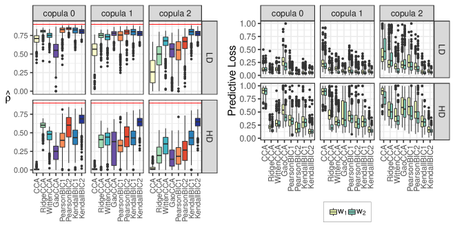
Figure 1: Truncated/truncated case. Left: The value of $\widehat{\rho}$ from (7). The horizontal lines indicate the true canonical correlation value $\rho=$ 0$\cdot$9. Right: The value of predictive loss (8). Results over 500 replications. CCA: Sample canonical correlation analysis; RidgeCCA: Canonical ridge of González et al. (2008); WittenCCA: method of Witten et al. (2009); GaoCCA: method of  Gao et al. (2017); PearsonBIC1, PearsonBIC2: proposed algorithm with Pearson sample correlation matrix; KendallBIC1, KendallBIC2: proposed algorithm with rank-based estimator $\widetilde{R}$; bic₁ or bic₂ refer to tuning parameter selection criteria; LD: low-dimensional setting ($p_{1}=p_{2}=25$); HD: high-dimensional setting ($p_{1}=p_{2}=100$).

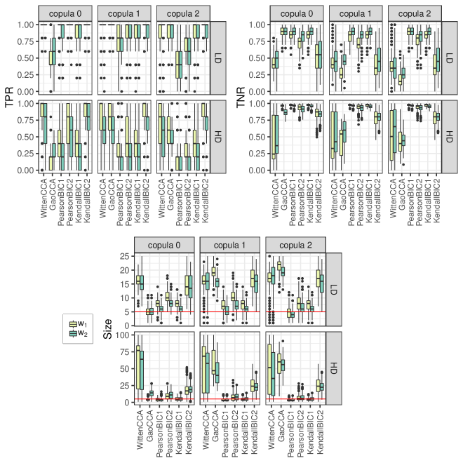
Figure 2: Truncated/truncated case. TopLeft: True positive rate (TPR); TopRight: True negative rate (TNR); BottomMiddle: Selected model size. Results over 500 replications. WittenCCA: method of Witten et al. (2009); GaoCCA: method of  Gao et al. (2017); PearsonBIC1, PearsonBIC2: proposed algorithm with Pearson sample correlation matrix; KendallBIC1, KendallBIC2: proposed algorithm with rank-based estimator $\widetilde{R}$; bic₁ or bic₂ refer to tuning parameter selection criteria; LD: low-dimensional setting ($p_{1}=p_{2}=25$); HD: high-dimensional setting ($p_{1}=p_{2}=100$).

The results for the truncated/truncated case over 500 replications are presented in Figures 1–2. From Figure 1, the majority of methods achieve higher values of $\widehat{\rho}$ in the absence of data transformation (copula 0) compared to cases where transformation is applied (copula 1 and 2). The only exception is our approach based on Kendall’s $\tau$, which as expected has comparable performance across the copula types. The performance of all methods deteriorates with increased dimension leading to smaller values of $\widehat{\rho}$ and larger predictive losses. The classical canonical correlation analysis performs especially poorly in high-dimensional settings with $\widehat{\rho}$ being almost 0 and predictive loss being close to 1 for both $w_{1}$ and $w_{2}$. Canonical ridge works well in the copula 0 setting, however its performance is strongly affected in the presence of transformations (copula 1 and 2). Surprisingly to us, Gao’s method, as implemented in SCCALab, performs poorly compared to other approaches. Since Gao’s method is designed for Gaussian data, the poor performance is likely due to its sensitivity to the presence of copulas and zero truncation (in the copula 0 case, proportions of zero values for each variable range from $5\%$ to $70\%$). We also use the default values in SCCALab for all of the parameters, so better performance could possibly be achieved by adjusting those values. Sparse canonical correlation analysis based on Pearson’s correlation outperforms all other methods in low dimensional setting when no data transformation is applied (copula 0), however its performance deteriorates when the monotone transformations are applied to the data (copulas 1 and 2). It also performs worse than our rank-based approach in high-dimensional setting. This is likely due to the increase in variables with zero inflation due to truncation, which Pearson’s correlation doesn’t take into account. In low-dimensional settings, bic₁ and bic₂ criteria lead to similar values of $\widehat{\rho}$, with larger variance in bic₁ performance. In high-dimensional settings, bic₂ is clearly better than bic₁ in predictive performance, and this better performance is irrespective of the choice of the estimator for the latent correlation matrix (Pearson’s correlation matrix or proposed rank-based correlation matrix). Overall, our method based on Kendall’s $\tau$ with bic₂ criterion leads to highest values of $\widehat{\rho}$ and smallest values of predictive loss across dimensions and different copula types.

Figure 2 illustrates variable selection performance of each method. The classical canonical correlation analysis and canonical ridge are excluded as they do not perform variable selection. To ensure the results are consistent with numerical precision of optimization algorithm, we treat variable as nonzero if its loading is above $10^{-6}$ threshold in absolute value. Unexpected to us, the number of selected variables varies significantly across replications for Witten’s method (bottom figure in Figure 2), leading to significant variations in true positive and true negative rates. We suspect this is due to the use of a permutation approach for selection of tuning parameters. Our approach based on Kendall’s $\tau$ leads to a more favorable combination of true positive and true negative rates compared to competing methods, especially when data transformations are applied. Furthermore, this advantage is maintained independently of tuning parameter selection scheme. In Section S3$\cdot$3 of the Supplementary Material, we compare the true positive versus false positive curves obtained by each method over the range of tuning parameters, and find that our rank-based estimator leads to highest area under the curve in the copula settings. Comparing bic₁ with bic₂ performance in Figure 2, bic₁ leads to the sparsest model and the highest true negative rate for both Pearson correlation and our rank-based correlation , at the expense of missing some true variables in the high-dimensional settings. Given the comparison in predictive performance between the two selection criteria, we conclude that bic₁ is better suited for variable selection, especially when it is desired to have a high true negative rate, whereas bic₂ works better for prediction.

In addition to the truncated/truncated case, we also consider truncated/continuous and truncated/binary cases in Section S3$\cdot$4 of the Supplementary Material. The conclusions of methods’ comparison are similar to the truncated/truncated case. Overall, all the methods perform best in the truncated/continuous case and worst in the truncated/binary case, which is not surprising, since dichotomization of continuous variable leads to a loss of information, thus reducing the effective sample size.

5 Application to TCGA data

The Cancer Genome Atlas (TCGA) project collects data from multiple platforms using high-throughput sequencing technologies. We consider gene expression data ($p_{1}=891$) and micro RNA data ($p_{2}=431$) for $n=500$ matched subjects from the TCGA breast cancer database. We treat gene expression data as continuous and micro RNA data as truncated continuous. The range of proportions of zero values contained in each variable in micro RNA data is $0-\text{49$\cdot$8}\%$. The subjects belong to one of the 5 breast cancer subtypes: Normal, Basal, Her2, LumA and LumB, with 37 subjects having missing subtype information (denoted as NA). The goal of the analysis is to characterize the association between gene expression and micro RNA data, and investigate whether this association is related to breast cancer subtypes.

To investigate the performance of our method relative to other approaches, we randomly split the data 500 times. Each time $400$ samples are used for training, and the remaining $100$ test samples are used to assess the association via

$$\widehat{\rho}_{\text{test}}=\left|\dfrac{\widehat{w}_{1,\text{train}}^{\top}\Sigma_{12,\text{test}}\widehat{w}_{2,\text{train}}}{(\widehat{w}_{1,\text{train}}^{\top}\Sigma_{1,\text{test}}\widehat{w}_{1,\text{train}})^{1/2}(\widehat{w}_{2,\text{train}}^{\top}\Sigma_{2,\text{test}}\widehat{w}_{2,\text{train}})^{1/2}}\right|.$$

Here $\Sigma_{\text{test}}$ is evaluated based on the test samples, and is either the rank-based estimator $\widetilde{R}$ for our method, or the sample covariance matrix for other methods. We also compare the number of selected genes and selected micro RNAs, and the results are presented in Table 1. We have not considered the method of Gao et al. (2017) in this section due to its poor performance in Section 4 and high computational cost (it takes around 40 minutes per replication on these data on a Windows 3$\cdot$60GHz Intel Core i7 CPU machine).

Method	Selected Genes				Selected micro RNAs				$\widehat{\rho}_{\text{test}}$
CCA			891$\cdot$00	(0$\cdot$00)			431$\cdot$00	(0$\cdot$00)		0$\cdot$004	(0$\cdot$109)
RidgeCCA			891$\cdot$00	(0$\cdot$00)			431$\cdot$00	(0$\cdot$00)		0$\cdot$712	(0$\cdot$126)
WittenCCA			338$\cdot$36	(194$\cdot$58)			165$\cdot$53	(100$\cdot$30)		0$\cdot$789	(0$\cdot$041)
PearsonBIC1			9$\cdot$92	(2$\cdot$62)			16$\cdot$08	(3$\cdot$18)		0$\cdot$813	(0$\cdot$044)
PearsonBIC2			27$\cdot$68	(6$\cdot$20)			40$\cdot$50	(12$\cdot$54)		0$\cdot$857	(0$\cdot$034)
KendallBIC1			18$\cdot$24	(3$\cdot$51)			9$\cdot$68	(3$\cdot$15)		$\mathbf{0}$$\cdot$$\mathbf{880}$	(0$\cdot$030)
KendallBIC2			38$\cdot$18	(8$\cdot$47)			31$\cdot$01	(6$\cdot$74)		$\mathbf{0}$$\cdot$$\mathbf{913}$	(0$\cdot$029)

Table 1: Mean support sizes and values of $\widehat{\rho}_{\text{test}}$’s over 500 random splits of breast cancer data. The standard deviation is given in parentheses

Of course, neither the sample canonical correlation analysis nor the canonical ridge method performs variable selection. In addition, $\widehat{\rho}_{\text{test}}$ is very close to $0$ for the sample canonical correlation, confirming poor performance of the method. Canonical ridge leads to significantly higher values of $\widehat{\rho}_{\text{test}}$ demonstrating the advantage of added regularization, however it still has smaller correlation values compared to other approaches. The method of Witten et al. (2009) leads to higher correlation values compared to both sample canonical correlation analysis and canonical ridge, however it still selects a significant number of variables, with highly variable model sizes across replications. We suspect this is due to the use of a permutation-based algorithm for tuning parameter selection: similar behaviour is also observed in Section 4. Sparse canonical correlation analysis based on Pearson’s correlation selects a much smaller number of genes and micro RNAs but achieves higher values of $\widehat{\rho}_{\text{test}}$ than the method of Witten et al. (2009). This is consistent with results in Section 4. The highest values of $\widehat{\rho}_{\text{test}}$ are achieved by our approach based on Kendall’s $\tau$ with smaller number of selected variables, confirming that found association is not due to over-fitting as it generalizes well to out-of-sample data. bic₁ criterion leads to the sparser model than bic₂ consistently for both Pearson and Kendall-based correlation estimates, with bic₂ criterion having the larger out-of-sample correlation value. In light of these results and results of Section 4, we conclude that bic₁ is advantageous for variable selection due to its selection of sparser model and higher true negative rate observed in simulations, whereas bic₂ is advantageous for prediction.

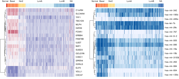
Figure 3: Genes and micro RNAs selected often more than 80% of 500 repetitions by our approach with the bic₂ criterion are used for heatmap. Left: A heatmap of 19 genes. The blue indicates positive expression level, and red for negative expression level. The white means zero expression level. Right: A heatmap of 16 micro RNAs. The saturation level of colors are assigned based on variable-specific quantiles. For both figures, the dissimilarity measure is set as $1-\widetilde{R}$ with our rank-based correlation $\widetilde{R}$, and Ward linkage is used.

We next investigate possible relationships between selected variables and breast cancer subtypes. Since the selected variables may change across the random data splits, we consider the selection frequency of each gene and micro RNA across all 500 replications of our method with bic₂ criterion, and choose the variables that are selected at least 80% of the times. Figure 3 shows heatmaps of expression levels of resulting 19 genes and 16 micro RNAs, with samples ordered by their respective cancer subtype. The heatmaps show clear separation between Basal and other subtypes, suggesting that the found association is relevant to cancer biology.

Many of the selected genes and micro RNAs can be found in recent literature which supports their association with breast cancer. Kim et al. (2016) indicates that ERBB4 is a prognostic marker for triple negative breast cancer, which is often used interchangeably with Basal-like breast cancer. In agreement with our results, Castilla et al. (2014) identifies that VGLL1 and miR-934 are highly correlated with each other, and that both are overexpressed in the Basal-like subtype. They also find that selected FOXA1 and GATA3 genes, as well as ESR1 gene (not selected at 80% frequency threshold, but still has a 73.4% frequency), have strong negative correlation with both VGLL1 and miR-934. The expression level of selected ELF5 is shown to play a key role in determining breast cancer molecular subtype in Kalyuga et al. (2012) and Piggin et al. (2016). Furthermore, Jonsdottir et al. (2012) validate that selected hsa-miR-18a and hsa-miR-505 miRNAs are significantly correlated with prognostic breast cancer biomarkers, and high expression of hsa-miR-18a is strongly associated with Basal-like breast cancer features. Finally, the selected hsa-miR-135b is reported to be related to breast cancer cell growth in Aakula et al. (2015) and Hua et al. (2016).

6 Discussion

One of the main contributions of this work is a truncated Gaussian copula model for the zero-inflated data, and corresponding development of a rank-based estimator for the latent correlation matrix. While our focus is on canonical correlation analysis, our estimator can be used in conjunction with other covariance-based approaches. For example it can be used for constructing graphical models as in Fan et al. (2017) in cases where some or all of the variables have an excess of zeros. Micro RNA data is one example that we have explored in this work, however another prominent example is microbiome abundance data. It would be of interest to further explore the potential of our modeling approach in different application areas. The R package mixedCCA with our method’s implementation is available from the authors github page https://github.com/irinagain/mixedCCA.

References

- Aakula et al. (2015) Aakula, A., Leivonen, S.-K., Hintsanen, P., Aittokallio, T., Ceder, Y., Børresen-Dale, A.-L., Perälä, M., Östling, P. & Kallioniemi, O. (2015). MicroRNA-135b regulates ER, AR and HIF1AN and affects breast and prostate cancer cell growth. Molecular Oncology 9, 1287–1300.
- Agniel & Cai (2017) Agniel, D. & Cai, T. (2017). Analysis of multiple diverse phenotypes via semiparametric canonical correlation analysis. Biometrics 73, 1254–1265.
- Bach & Jordan (2005) Bach, F. R. & Jordan, M. I. (2005). A probabilistic interpretation of canonical correlation analysis. Tech. Rep. 688, Department of Statistics, University of California, Berkeley.
- Boyd & Vandenberghe (2004) Boyd, S. P. & Vandenberghe, L. (2004). Convex Optimization. Cambridge: Cambridge Univ Press.
- Castilla et al. (2014) Castilla, M. Á., López-García, M. Á., Atienza, M. R., Rosa-Rosa, J. M., Diaz-Martin, J., Pecero, M. L., Vieites, B., Romero-Pérez, L., Benítez, J., Calcabrini, A. & Palacios, J. (2014). VGLL1 expression is associated with a triple-negative basal-like phenotype in breast cancer. Endocrine-Related Cancer 21, 587 – 599.
- Chen et al. (2013) Chen, M., Gao, C., Ren, Z. & Zhou, H. H. (2013). Sparse CCA via precision adjusted iterative thresholding. arXiv , 1311.6186v1.
- Chen & Liu (2011) Chen, X. & Liu, H. (2011). An efficient optimization algorithm for structured sparse cca, with applications to eQTL mapping. Statistics in Biosciences 4, 3–26.
- Chi et al. (2013) Chi, E. C., Allen, G. I., Zhou, H., Kohannim, O., Lange, K. & Thompson, P. M. (2013). Imaging genetics via sparse canonical correlation analysis. In 2013 IEEE 10th International Symposium on Biomedical Imaging.
- Cruz-Cano & Lee (2014) Cruz-Cano, R. & Lee, M.-L. T. (2014). Fast regularized canonical correlation analysis. Computational Statistics & Data Analysis 70, 88–100.
- Fan et al. (2017) Fan, J., Liu, H., Ning, Y. & Zou, H. (2017). High dimensional semiparametric latent graphical model for mixed data. J. R. Statist. Soc. B 79, 405–421.
- Gao et al. (2015) Gao, C., Ma, Z., Ren, Z. & Zhou, H. H. (2015). Minimax estimation in sparse canonical correlation analysis. Annals of Statistics 43, 2168–2197.
- Gao et al. (2017) Gao, C., Ma, Z. & Zhou, H. H. (2017). Sparse CCA: Adaptive estimation and computational barriers. Annals of Statistics 45, 2074–2101.
- González et al. (2008) González, I., Déjean, S., Martin, P. G. & Baccini, A. (2008). CCA: An R package to extend canonical correlation analysis. Journal of Statistical Software 23, 1–14.
- Gorski et al. (2007) Gorski, J., Pfeuffer, F. & Klamroth, K. (2007). Biconvex sets and optimization with biconvex functions: a survey and extensions. Mathematical Methods of Operations Research 66, 373–407.
- Guo et al. (2016) Guo, Y., Ding, X., Liu, C. & Xue, J.-H. (2016). Sufficient canonical correlation analysis. IEEE Transactions on Image Processing 25, 2610–2619.
- Hardoon et al. (2004) Hardoon, D. R., Szedmak, S. & Shawe-Taylor, J. (2004). Canonical correlation analysis: An overview with application to learning methods. Neural Computation 16, 2639–2664.
- Hotelling (1936) Hotelling, H. (1936). Relations between two sets of variates. Biometrika 28, 321–377.
- Hua et al. (2016) Hua, K., Jin, J., Zhao, J., Song, J., Song, H., Li, D., Maskey, N., Zhao, B., Wu, C., Xu, H. et al. (2016). miR-135b, upregulated in breast cancer, promotes cell growth and disrupts the cell cycle by regulating LATS2. International Journal of Oncology 48, 1997–2006.
- Jonsdottir et al. (2012) Jonsdottir, K., Janssen, S. R., Da Rosa, F. C., Gudlaugsson, E., Skaland, I., Baak, J. P. A. & Janssen, E. A. M. (2012). Validation of expression patterns for nine miRNAs in 204 lymph-node negative breast cancers. PLOS ONE 7, 1–9.
- Kalyuga et al. (2012) Kalyuga, M., Gallego-Ortega, D., Lee, H. J., Roden, D. L., Cowley, M. J., Caldon, C. E., Stone, A., Allerdice, S. L., Valdes-Mora, F., Launchbury, R., Statham, A. L., Armstrong, N., Alles, M. C., Young, A., Egger, A., Au, W., Piggin, C. L., Evans, C. J., Ledger, A., Brummer, T., Oakes, S. R., Kaplan, W., Gee, J. M. W., Nicholson, R. I., Sutherland, R. L., Swarbrick, A., Naylor, M. J., Clark, S. J., Carroll, J. S. & Ormandy, C. J. (2012). ELF5 suppresses estrogen sensitivity and underpins the acquisition of antiestrogen resistance in luminal breast cancer. PLOS Biology 10, 1–17.
- Kim et al. (2016) Kim, J.-Y., Jung, H. H., Do, I.-G., Bae, S., Lee, S. K., Kim, S. W., Lee, J. E., Nam, S. J., Ahn, J. S., Park, Y. H. et al. (2016). Prognostic value of ERBB4 expression in patients with triple negative breast cancer. BMC Cancer 16, 138.
- Liu et al. (2009) Liu, H., Lafferty, J. & Wasserman, L. (2009). The nonparanormal: Semiparametric estimation of high dimensional undirected graphs. Journal of Machine Learning Research 10, 2295–2328.
- Mai & Zhang (2019) Mai, Q. & Zhang, X. (2019). An iterative penalized least squares approach to sparse canonical correlation analysis. Biometrics 75, 734–744.
- Parkhomenko et al. (2009) Parkhomenko, E., Tritchler, D. & Beyene, J. (2009). Sparse canonical correlation analysis with application to genomic data integration. Statistical Applications in Genetics and Molecular Biology 8, 1–34.
- Piggin et al. (2016) Piggin, C. L., Roden, D. L., Gallego-Ortega, D., Lee, H. J., Oakes, S. R. & Ormandy, C. J. (2016). ELF5 isoform expression is tissue-specific and significantly altered in cancer. Breast Cancer Research 18, 4.
- Reid et al. (2016) Reid, S., Tibshirani, R. & Friedman, J. (2016). A study of error variance estimation in lasso regression. Statistica Sinica 26, 35–67.
- Safo et al. (2018) Safo, S. E., Li, S. & Long, Q. (2018). Integrative analysis of transcriptomic and metabolomic data via sparse canonical correlation analysis with incorporation of biological information. Biometrics 74, 300–312.
- Tibshirani (1996) Tibshirani, R. (1996). Regression shrinkage and selection via the lasso. J. R. Statist. Soc. B 58, 267–288.
- Tibshirani & Taylor (2012) Tibshirani, R. J. & Taylor, J. (2012). Degrees of freedom in lasso problems. Annals of Statistics 40, 1198–1232.
- Tseng (1988) Tseng, P. (1988). Coordinate ascent for maximizing nondifferentiable concave functions. Tech. rep., Massachusetts Institute of Technology, Laboratory for Information and Decision Systems.
- Wilms & Croux (2015) Wilms, I. & Croux, C. (2015). Sparse canonical correlation analysis from a predictive point of view. Biometrical Journal 57, 834–851.
- Witten & Tibshirani (2009) Witten, D. M. & Tibshirani, R. J. (2009). Extensions of sparse canonical correlation analysis with applications to genomic data. Statistical Applications in Genetics and Molecular Biology 8, 1–27.
- Witten et al. (2009) Witten, D. M., Tibshirani, R. J. & Hastie, T. (2009). A penalized matrix decomposition, with applications to sparse principal components and canonical correlation analysis. Biostatistics 10, 515–534.
- Zoh et al. (2016) Zoh, R. S., Mallick, B., Ivanov, I., Baladandayuthapani, V., Manyam, G., Chapkin, R. S., Lampe, J. W. & Carroll, R. J. (2016). PCAN: Probabilistic correlation analysis of two non-normal data sets. Biometrics 72, 1358–1368.