Rebalancing Frequency Considerations for Kelly-Optimal
Stock Portfolios in a Control-Theoretic Framework
Abstract
In this paper, motivated by the celebrated work of Kelly, we consider the problem of portfolio weight selection to maximize expected logarithmic growth. Going beyond existing literature, our focal point here is the rebalancing frequency which we include as an additional parameter in our analysis. The problem is first set in a control-theoretic framework, and then, the main question we address is as follows: In the absence of transaction costs, does high-frequency trading always lead to the best performance? Related to this is our prior work on betting, also in the Kelly context, which examines the impact of making a wager and letting it ride. Our results on betting frequency can be interpreted in the context of weight selection for a two-asset portfolio consisting of one risky asset and one riskless asset. With regard to the question above, our prior results indicate that it is often the case that there are no performance benefits associated with high-frequency trading. In the present paper, we generalize the analysis to portfolios with multiple risky assets. We show that if there is an asset satisfying a new condition which we call dominance, then an optimal portfolio consists of this asset alone; i.e., the trader has “all eggs in one basket” and performance becomes a constant function of rebalancing frequency. Said another way, the problem of rebalancing is rendered moot. The paper also includes simulations which address practical considerations associated with real stock prices and the dominant asset condition.
I Introduction
The main results of this paper pertain to the effect of “rebalancing frequency” for portfolio weight selection problems with performance measured using Kelly’s celebrated expected logarithmic growth criterion, which was first used for a variety of sequential betting problems [1]; see also [2]-[7] where further results along these lines are given. In this regard, the work reported in this paper is part of a line of research using this criterion in the context of portfolio optimization in the stock market; e.g., see [8] and [9] for a good introduction, [10] for a rather comprehensive exposition on the properties of solutions obtained using expected logarithmic growth, and [11]-[17] for a sampling of some more recent developments. Initial results about rebalancing frequency are reported in [11] and [12] for the case when the stock prices follow a continuous-time geometric Brownian motion. Additionally, a drawback in [12] is that the betting fraction is chosen without regard to the frequency at which the portfolio is rebalanced. Subsequently, when this same fraction is used to find an optimal rebalancing period, the resulting levels of logarithmic growth are suboptimal. To complete this overview, we single out [17] for emphasis since it provides a comprehensive survey covering many of the most important papers in this line of research.
Most closely related to this paper is our recent work [21] which considers a repeated betting game and the impact on expected logarithmic growth resulting from making a wager and letting it ride for several steps in lieu of updating. This can be interpreted as weight selection for a two-asset portfolio and “letting it ride” to capture the effect of the frequency of rebalancing. With this as background, this paper is aimed at generalizing these initial results on frequency dependence to trading a multi-stock portfolio.
The appeal of this research to the control community is based on the fact that the Kelly-based rebalancing problem can be formulated as a stochastic control problem with a linear feedback and randomly varying inputs corresponding to the vector of stagewise returns on portfolio assets; see [15]-[16], [18]-[20], and [22] where a similar control-theoretic set-up is considered for finance problems in continuous time. To study the effect of rebalancing frequency for portfolio problems, let be the time between portfolio updates. With being the number of steps between rebalancings, the frequency is
Subsequently, for each , the expected logarithmic growth using optimal portfolio weights is denoted by , which we study as a function of .
The main questions we address in this paper are as follows: Does high-frequency trading, corresponding to , always lead to the best performance? Under what conditions can a low-frequency trader using match or exceed the optimal high-frequency performance level ? Indeed, in the presence of transaction costs, our previous work mentioned above, carried out in the context of sequential betting, includes a demonstration that is possible when transaction costs are in play. That is, the prohibitive costs associated with trading too often may render high-frequency trading suboptimal. However, for the zero transaction-cost case, we also showed that it is possible to obtain for all although it is still an open question whether is possible. For this case, in the sequel, we generalize these results in [21] to the multiple-risky-asset case, and prove that there are many scenarios where the low-frequency trader’s performance can actually match that of the high-frequency trader — the extreme case with very large corresponding to buy and hold. This performance matching is proven when at least one of the assets in the portfolio is dominant in the sense that it is relatively more attractive than every other potential asset under consideration. In this case, it becomes arguable that dynamic portfolio rebalancing is a “waste of time” to even consider.
To complete this overview, we should also mention another result in the literature involving rebalancing frequency considerations. In [11], the returns are assumed to follow a continuous-time geometric Brownian motion and two extreme cases are considered — when the time between rebalancing is either very large or very small. In contrast to [11], we consider the entire range of frequencies from low to high. To this end, our objective here is to analyze, in discrete time, the more general case when both the probability distribution of the returns and the time interval between updates are arbitrary.
Preview of Main Result: For the case when the portfolio is comprised of two or more potentially investable assets with each having i.i.d. returns and possibly correlated, Asset is said to be dominant if
holds for all . In this case, our main result, which we call the Dominant Asset Theorem, tells us that when this condition is satisfied, an optimal strategy is obtained by investing all of the trader’s funds in Asset . Figuratively speaking, this result says that an optimal portfolio is obtained by putting all eggs in one basket. Of equal importance, as a consequence of the theorem, it is seen that the performance of the high-frequency trader and the buy and holder are identical. That is, for all . Thus, performance is invariant to the rebalancing frequency and it follows that there is no benefit associated with trading often; it suffices to buy and hold. Said another way, if all funds are invested in a single asset, which could be cash, then rebalancing is rendered moot. Equivalently, the performance must be a constant function of .
Theoretical Versus Practical Considerations: Consistent with the vast preponderance of results in the literature, our approach is model based in the sense that the probability distribution for the asset returns is known; see Section II for details. The reader is also referred to [8] and [24] where binomial lattice models are used to approximate geometric Brownian motion. In practice, the probability distribution of the returns is typically estimated from historical data. In view of the fact that real-world stock returns are generally nonstationary, in practice, frequent updates of the model accompanied by portfolio rebalancing are in order. That is, at best, model-based results should be viewed as useful only for a limited amount of time. In Section V, the reader is provided with the flavor of these practical issues in the context of the dominance result described above.
II Control-Theoretic Formulation
In this section, we begin with a trader who is forming a portfolio and considering potential assets for inclusion. We now formulate the frequency-dependent portfolio problem in control-theoretic terms. Indeed, the system output at stage is taken to be the trader’s time-varying account value for and, for , we use feedback gains to represent the fraction of this amount allocated to the -th asset. The inequality means that the trader is going long and short selling is disallowed. In addition, forces the amount invested to be no more than the account value . In other words, this disallows the use of leverage and possible margin costs. This no-leverage requirement, applied to the portfolio in its entirety, leads to the constraint
That is, with , we have a guarantee that no more than 100% of the account value is invested; see the conclusion for further discussion. Now, the -th control signal is a linear feedback of the form
which is called the -th investment function.
The Asset Returns: If Asset is a stock whose price at time is , then its return is
In the sequel, we assume a “perfect model” for the stochastic process driving the stock prices. That is, for risky assets, we assume that the return vectors have a known distribution with components which can be arbitrarily correlated. It is also assumed that these vectors are independent and identically distributed (i.i.d.) with components satisfying
with known bounds above and with being finite and . This means that the loss per time step is limited to less than and is interpreted to mean that the price of a stock cannot drop to zero. To avoid triviality, we assume that at least one of the assets is riskless with nonnegative rate of return . That is, if Asset is riskless, its return is deterministic and is treated as a degenerate random variable for all with probability one. The quantity is called an interest rate, and it is noted that this formulation also allows for the trader to maintain cash in the account by taking 111 There are rare cases when the best possible riskless asset has negative returns and the optimal portfolio, which will be discussed in Section IV, might be one which involves losing money as slowly as possible.
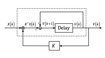
Dynamics and Trading Frequency Considerations: The update in account value from stage to for the resulting closed-loop system, depicted in Figure 1, is
Letting be the number of steps between rebalancings, at time , the trader begins with investment and waits steps in the spirit of “buy and hold.” Then, when , the investment is updated to be
Continuing in this manner, a waiting period of stages is enforced between each rebalance. Now, to study performance as a function of frequency, we use the compound returns
which are readily seen to satisfy for all and . In the sequel, we work with the random vector having -th component . Then, for any fixed rebalancing period and initial account value , the corresponding account value at stage is given by
The Frequency Dependent Optimization Problem: As a function of , we study the problem of maximizing the expected logarithmic growth
which is concave in . The associated optimal expected logarithmic growth is obtained as
and any satisfying is called an optimal Kelly fraction for the rebalancing period of length .
III Relative Attractiveness and Dominance
As discussed in Section I, in our prior work [21], the Kelly betting problem results can be interpreted in the context of weight selection for a two-asset portfolio consisting of one risky asset and one riskless asset. We proved that under a simple condition which we called “sufficient attractiveness,” is a constant function of . Thus, when this condition holds, trading faster does not lead to performance improvement over a simple buy-and-hold strategy. To extend these results to the case of a portfolio of arbitrary size , we generalize the notion of sufficient attractiveness with the definition below.
Definition (Relative Attractiveness and Dominance): Given a collection of assets, we say that Asset is relatively more attractive than Asset if
Equivalently, Asset is relatively more attractive than Asset if the correlation between and is at most one. Asset is said to be dominant if it is relatively more attractive than every other asset .
Remarks: When , we note that Asset is dominant if and only if it is relatively more attractive than Asset . If and Asset is riskless with , then the dominance of Asset is equivalent to its sufficient attractiveness as defined in [21]. If , a riskless Asset with interest rate is easily seen to be relatively more attractive than risky Asset if and only if
For a risky Asset to be relatively more attractive than the riskless Asset , we require more than just . For example, consider returns with
Then with , a straightforward calculation leads to
but
which violates the relative attractiveness inequality. Although the condition is not sufficient for a risky Asset to be relatively more attractive than a riskless Asset , the condition is necessary. This can be seen by applying Jensen’s inequality to obtain
If Asset is relatively more attractive than riskless Asset , then the right hand side above is one at most, and we obtain
from which it follows that
Thus, is necessary, but not sufficient for risky Asset to be relatively more attractive than riskless Asset . The reader should not confuse the definition of dominant asset with the definition of stochastic dominance. Recall that stochastic dominance involves only the marginal distributions of two random variables, while the dominant asset definition involves the correlation between and , which depends on the joint distribution of and .
IV Dominant Asset Theorem
The theorem below tells us that the satisfaction of the dominant asset inequality leads to an optimal portfolio which involves investing 100% of available funds in a single asset. In other words, if an asset is dominant, “bet the farm” on it.
Dominant Asset Theorem: Given a collection of assets, if Asset is dominant, then, for all , is maximized by
where is the unit vector in the -th coordinate direction. Furthermore, the resulting optimal expected logarithmic growth rate is given by
Proof: In order to prove , it suffices to show that for . For notational convenience, we work with the random vector
representing the total return with -th component . Letting , since for , it follows that
Hence, by applying Jensen’s inequality to the concave logarithm function above, we obtain a chain of inequalities
where the last inequality follows from the dominance of Asset and the fact that . Now, since , it follows that
and
To complete the proof, it remains to show that . This is easily obtained by recalling that the are i.i.d. and observing that
V Application to Stock-Market Data
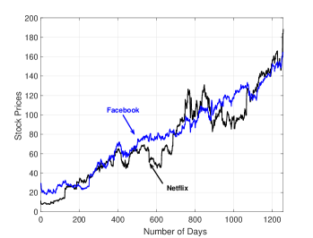
Per discussion in the introduction, in this section, our objective is to illustrate some of the practical issues which arise when studying asset domination using historical data. To this end, we consider three assets as portfolio candidates. Asset 1 is Netflix (ticker: NFLX), Asset 2 is Facebook (ticker: FB) and Asset 3 is a riskless asset with daily interest rate . We consider the problem of rebalancing our positions in these assets over a four-year period beginning on January 24, 2013. We work with the adjusted daily closing prices for this period and demonstrate how the Dominant Asset Theorem might apply in practice. The price plot for the two stocks in Figure 2 begins with the 126-day period prior to the start of trading. This data was used as a “training set” to initialize the analysis to follow.
Given the fact that a practitioner should rightfully view the stochastic process model for the stock returns as nonstationary, when testing for satisfaction of the relative attractiveness inequality, we work with a sliding window consisting of the most recent trading days. Hence, at day , we use an empirical estimate of the expected value for the attractiveness ratio involving the -th and -th assets which is given by
The simulations to follow use a window size of which corresponds to about six months. Beginning with the initial condition established using the training set, we generate the over the period of interest. In view of the nonstationarity of the returns, as seen in the simulation to follow, the are time-varying. Hence, an asset which is dominant at some point in time may no longer be dominant at a later time.
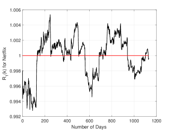
With the considerations above, we begin our analysis with and consider the following two questions. Question 1: In a zero interest rate environment, over what time periods is Netflix the dominant asset? During such periods, in accordance with the theorem, the trader is non-diversified with the entire portfolio in Netflix. Question 2: At stage , how large must the interest rate be so that the riskless asset is dominant? That is, when the interest rate is suitably high, our theory dictates that the trader has a portfolio which is 100% in fixed income with no positions in Netflix and Facebook.
To answer the first question, we provide a plot of
versus in Figure 3, and, consistent with the theorem, we deem Netflix to be dominant over the subset of time periods for which Over the periods when , there are various additional scenarios which can be studied with the given data. For example, sometimes there is no dominant asset and at other times either Facebook or the riskless asset is dominant.
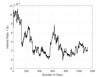
To answer the second question, we begin with the following observation: The theorem tells us that Asset 3, the riskless asset, is dominant if and only if
Again taking the nonstationarity of the data into account, we let denote the estimated value of the left hand size above based on the most recent -day window. That is, we take
In Figure 4, we see that there are time periods when the market is performing quite well and it takes a remarkably high interest rate in order to forego investing in the stocks.
VI Conclusion and Future Work
In this paper, we showed that if an asset is dominant, an optimal trading strategy is to invest all available funds into it. For such cases, rebalancing becomes moot and the trading performance, namely , is a constant. It is also worth mentioning that the paradigm presented in this paper remains valid for a wide variety of other choices for the admissible feedback gain set associated with leveraged investments with some components . For example, in [16], this is achieved by imposing a “survival” constraint which disallows any trade that can potentially lead to .
Regarding further research, one obvious continuation would be to study the case when is allowed. As mentioned in Section II, this corresponds to short selling. In this situation, we envision a similar definition of dominant asset and results along the lines of those given here. A second direction for further work involves the case when no dominant asset exists, Might it ever be true that ? We believe that an affirmative answer to this question would be important. It would tell us that a low-frequency trader such as a buy and holder might strictly outperform the high-frequency trader.
Finally, it would be important to develop new results on Kelly-based trading which do not rely knowledge of a perfect stochastic model for the returns . For cases when the model is either partially known or completely unknown, we plan to investigate the extent to which the theory in this paper can be extended. Our preliminary work along these lines suggests that there may be a more general version of the Dominant Asset Theorem which is established using asymptotic analysis to obtain performance guarantees for suitably large.
References
- [1] J. L. Kelly, “A New Interpretation of Information Rate,” Bell System Technical Journal, vol. 35.4, pp. 917-926, 1956.
- [2] H. A. Latané, “Criteria for Choice Among Risky Ventures,” Journal Political Economy, vol. 67, pp. 144-155, 1959.
- [3] L. Breiman, “Optimal Gambling Systems for Favorable Games.” Proceedings of the 4th Berkeley Symposium on Mathematical Statistics and Probability, vol 1, pp. 63-68, 1961.
- [4] N. H. Hakansson, “On Optimal Myopic Portfolio Policies With and Without Serial Correlation,” Journal of Business, vol. 44, pp. 324-334, 1972.
- [5] E. O. Thorp, “Optimal Gambling Systems for Favorable Games,” Review of The International Statistical Institute, vol. 37, pp. 273-293, 1969.
- [6] P. H. Algoet and T. M. Cover, “Asymptotic Optimality and Asymptotic Equipartition Properties of Log-Optimum Investment,” The Annals of Probability, vol. 16, pp. 876-898, 1988.
- [7] T. M. Cover and J. A. Thomas, Elements of Information Theory, John Wiley and Sons, 2012.
- [8] D. G. Luenberger, Investment Science, Oxford University Press, New York, 2011.
- [9] E. O. Thorp, “The Kelly Criterion in Blackjack Sports Betting and The Stock Market,” Handbook of Asset and Liability Management: Theory and Methodology, vol. 1, pp. 385-428, Elsevier Science, 2006.
- [10] L. C. Maclean, E. O. Thorp, and W. T. Ziemba “Long-term Capital Growth: The Good and Bad Properties of The Kelly and Fractional Kelly Capital Growth Criteria,” Quantitative Finance, vol. 10, pp. 681-687, 2010.
- [11] D. Kuhn and D. G. Luenberger, “Analysis of the Rebalancing Frequency in Log-Optimal Portfolio Selection,” Quantitative Finance, vol. 10, pp. 221-234, 2010.
- [12] S. R. Das, D. Kaznachey and M. Goyal, “Computing Optimal Rebalance Frequency for Log-Optimal Portfolios,” Quantitative Finance, vol. 14, pp.1489-1502, 2014.
- [13] V. Nekrasov, “Kelly Criterion for Multivariate Portfolios: A Model-Free Approach,” Social Science Research Network, 2014.
- [14] A. W. Lo, H. A. Orr, and R. Zhang “The Growth of Relative Wealth and the Kelly Criterion,” Social Science Research Network, 2017.
- [15] C. H. Hsieh and B. R. Barmish, “On Kelly Betting: Some Limitations,” Proceedings of the Allerton Conference on Communication, Control, and Computing, pp. 165-172, Monticello, 2015.
- [16] C. H. Hsieh, B. R. Barmish, and J. A. Gubner, “Kelly Betting Can be Too Conservative,” Proceedings of the IEEE Conference on Decision and Control, pp. 3695-3701, Las Vegas, 2016.
- [17] L. C. Maclean, E. O. Thorp, and W. T. Ziemba, The Kelly Capital Growth Investment Criterion: Theory and Practice, World Scientific Publishing Company, 2011.
- [18] G. C. Calafiore and B. Monastero, “Triggering Long-Short Trades on Indexes,” International Journal of Trade, Economics and Finance, vol. 1, pp. 289-296, 2010.
- [19] C. H. Hsieh and B. R. Barmish, “On Drawdown-Modulated Feedback in Stock Trading,” IFAC-PapersOnLine, vol. 50, no. 1 pp. 952-958, 2017.
- [20] C. H. Hsieh and B. R. Barmish, “On Inefficiency of Markowitz-Style Investment Strategies When Drawdown is Important,” Proceedings of the IEEE Conference on Decision and Control, pp. 3075-3080, Melbourne, Australia, 2017.
- [21] C. H. Hsieh, B. R. Barmish, and J. A. Gubner, “At What Frequency Should the Kelly Bettor Bet,” Proceedings of the IEEE American Control Conference, pp. 5485-5490, Milwaukee, 2018.
- [22] B. R. Barmish and J. A. Primbs, “On a New Paradigm for Stock Trading Via a Model-Free Feedback Controller,” IEEE Transactions on Automatic Control, AC-61, pp. 662-676, 2016.
- [23] J. A. Gubner, Probability and Random Processes for Electrical and Computer Engineers, Cambridge University Press, 2006.
- [24] J. Cox, S. Ross, and S. Rubinstein, “Option Pricing: A Simplified Approach,” Journal of Financial Economics, vol. 7, pp. 229-263, 1979.