A one-variable bracket polynomial for some Turk’s head knots

Abstract

We compute the Kauffman bracket polynomial of the three-lead Turk’s head, the chain sinnet and the figure-eight chain shadow diagrams. Each of these knots can in fact be constructed by repeatedly concatenating the same $\displaystyle 3$-tangle, respectively, then taking the closure. The bracket is then evaluated by expressing the state diagrams of the concerned $\displaystyle 3$-tangle by means of the Kauffman monoid diagram’s elements.

Keywords: bracket polynomial, tangle shadow, Kauffman state, flat sinnet.

1 Introduction

The present paper is a follow-up on our previous work which aims at collecting statistics on knot shadows [5]. We would like to establish the bracket polynomial for knot diagram generated by the $\displaystyle 3$-tangle shadows below:

$$\begin{array}[]{cccccccc}\includegraphics[width=32.52017pt,valign={c}]{genB1}&&\includegraphics[width=32.52017pt,valign={c}]{genB2}&&\includegraphics[width=32.52017pt,valign={c}]{genB3}\\ T&&C&&E\end{array}.$$ (1)

The knot diagrams under consideration are those obtained by repeatedly multiplying (or concatenating) the same $\displaystyle 3$-tangle, then taking the closure of the resulting $\displaystyle 3$-tangle (i.e., connecting the endpoints in a standard way, without introducing further crossings between the strands). Knots obtained from the $\displaystyle 3$-tangles pictured in (1) belong to the Ashley’s Turk’s head family [1, p. 226, Chap. 17]: the three-lead Turk’s head [1, #1305], the chain sinnet [1, #1374] and the figure-eight chain [1, #1376], respectively (e.g. see Figure 1).

$\displaystyle\begin{array}[]{cccccccc}\includegraphics[width=97.56714pt,valign={c}]{braid1}&&\includegraphics[width=97.56714pt,valign={c}]{braid2}&&\includegraphics[width=97.56714pt,valign={c}]{braid3}\\ \mbox{Three-lead Turk's head}&&\mbox{Chain sinnet}&&\mbox{Figure-eight chain}\end{array}$

Figure 1: Some flat Turk’s-head knot diagrams.

The remainder of this paper is arranged as follows. In section 2, we establish the expression of the bracket polynomial for any $\displaystyle 3$-tangle shadow diagram. Then in section 3, we apply those results to the flat sinnet Turk’s heads mentioned earlier.

2 The Kauffman bracket of a $\displaystyle 3$-tangle shadow

In this paper, the Kauffman bracket maps a shadow diagram $\displaystyle D$ to $\displaystyle\left<D\right>\in$ $\displaystyle\mathbb{Z}[x]$ and is constructed from the following rules:

• $\displaystyle\left<\bigcirc\right>=x$;

• $\displaystyle\left<\bigcirc\sqcup D\right>=x\left<D\right>$;

• $\displaystyle\left<\includegraphics[width=13.00806pt,valign={c}]{crossing}\right>=\left<\includegraphics[width=13.00806pt,valign={c}]{split_2}\right>+\left<\includegraphics[width=15.17828pt,valign={c}]{split_1}\right>$.

The diagram $\displaystyle\bigcirc$ in $\displaystyle(\mathbf{K1})$ represents that of a single loop, and the symbol $\displaystyle\sqcup$ in $\displaystyle(\mathbf{K2})$ denotes the disjoint union operation. Formula in $\displaystyle(\mathbf{K3})$ expresses the splitting of a crossing. Recall that the choice of such splittings for any single crossing is referred to as the so-called Kauffman state. Rules $\displaystyle(\mathbf{K1})$, $\displaystyle(\mathbf{K2})$ and $\displaystyle(\mathbf{K3})$ can be summarized by the summation which is taken over all the states for $\displaystyle D$, namely $\displaystyle\left<D\right>=\sum_{S}x^{|S|}$ , where $\displaystyle|S|$ gives the number of loops in the state $\displaystyle S$. Kauffman shows that the states elements of a $\displaystyle 3$-tangle diagram $\displaystyle B:=\includegraphics[width=21.68231pt,valign={c}]{3tangleB}$ are generated by the product of a loop and the following $\displaystyle 5$ elements of the $\displaystyle 3$-strand diagram monoid $\displaystyle\mathcal{D}_{3}$ [2, 8]:

$$\begin{array}[]{ccccccccc}\includegraphics[width=30.35657pt,valign={c}]{1_3}&&\includegraphics[width=32.52017pt,valign={c}]{U_1}&&\includegraphics[width=32.52017pt,valign={c}]{U_2}&&\includegraphics[width=32.52017pt,valign={c}]{r}&&\includegraphics[width=32.52017pt,valign={c}]{s}\\ 1_{3}&&U_{1}&&U_{2}&&r&&s\end{array}.$$

In other words, given a state $\displaystyle S$, there exist a nonnegative integer $\displaystyle k$ and an element $\displaystyle U$ in $\displaystyle\mathcal{D}_{3}$ such that one writes $\displaystyle S=\bigcirc^{k}\sqcup U$, where $\displaystyle\bigcirc^{k}=\bigcirc\sqcup\bigcirc\sqcup\cdots\sqcup\bigcirc$ denotes the disjoint union of $\displaystyle k$ loops [3, p. 100]. The bracket of the $\displaystyle 3$-tangle $\displaystyle B$ becomes $\displaystyle\left<B\right>=\sum_{S}\left<S\right>$, where $\displaystyle\left<S\right>=x^{|S|}\left<U\right>$ for certain $\displaystyle U\in\mathcal{D}_{3}$.

Therefore $\displaystyle\left<B\right>$ is a linear combination of the brackets $\displaystyle\left<1_{3}\right>$, $\displaystyle\left<U_{1}\right>$, $\displaystyle\left<U_{2}\right>$,$\displaystyle\left<r\right>$ and $\displaystyle\left<s\right>$, i.e., there exist five polynomials $\displaystyle a,b,c,d,e$ in $\displaystyle\mathbb{Z}[x]$ such that

$$\left<B\right>=a\left<1_{3}\right>+b\left<U_{1}\right>+c\left<U_{2}\right>+d\left<r\right>+e\left<s\right>.$$ (2)

Lemma 1.

Given two $\displaystyle 3$-tangles $\displaystyle B$ and $\displaystyle D$, we have

$$\displaystyle\left<BD\right> \displaystyle=a_{B}a_{D}\left<1_{3}\right>+\left(b_{B}a_{D}+\left(a_{B}+b_{B}x+d_{B}\right)b_{D}+\left(d_{B}x+b_{B}\right)e_{D}\right)\left<U_{1}\right>$$

$$\displaystyle\hphantom{=}+\left(c_{B}a_{D}+\left(a_{B}+c_{B}x+e_{B}\right)c_{D}+\left(c_{B}+e_{B}x\right)d_{D}\right)\left<U_{2}\right>$$

$$\displaystyle\hphantom{=}+\left(d_{B}a_{D}+\left(d_{B}x+b_{B}\right)c_{D}+\left(a_{B}+b_{B}x+d_{B}\right)d_{D}\right)\left<r\right>$$

$$\displaystyle\hphantom{=}+\left(e_{B}a_{D}+\left(c_{B}+e_{B}x\right)b_{D}+\left(a_{B}+c_{B}x+e_{B}\right)e_{D}\right)\left<s\right>.$$

.

Proof.

We first establish the states of $\displaystyle B$ leaving $\displaystyle D$ intact, and then in $\displaystyle D$:

$$\displaystyle\left<BD\right> \displaystyle=a_{B}a_{D}\left<1_{3}^{2}\right>+a_{B}b_{D}\left<1_{3}U_{1}\right>+a_{B}c_{D}\left<1_{3}U_{2}\right>+a_{B}D\left<1_{3}r\right>+a_{B}e_{D}\left<1_{3}s\right>$$

$$\displaystyle\hphantom{=}+b_{B}a_{D}\left<U_{1}1_{3}\right>+b_{B}b_{D}\left<U_{1}^{2}\right>+b_{B}c_{D}\left<U_{1}U_{2}\right>+b_{B}d_{D}\left<U_{1}r\right>+b_{B}e_{D}\left<U_{1}s\right>$$

$$\displaystyle\hphantom{=}+c_{B}a_{D}\left<U_{2}1_{3}\right>+c_{B}b_{D}\left<U_{2}U_{1}\right>+c_{B}c_{D}\left<U_{2}^{2}\right>+c_{B}d_{D}\left<U_{2}r\right>+c_{B}e_{D}\left<U_{2}s\right>$$

$$\displaystyle\hphantom{=}+d_{B}a_{D}\left<r1_{3}\right>+d_{B}b_{D}\left<rU_{1}\right>+d_{B}c_{D}\left<rU_{2}\right>+d_{B}d_{D}\left<r^{2}\right>+d_{B}e_{D}\left<rs\right>$$

$$\displaystyle\hphantom{=}+e_{B}a_{D}\left<s1_{3}\right>+e_{B}b_{D}\left<sU_{1}\right>+e_{B}c_{D}\left<sU_{2}\right>+e_{B}d_{D}\left<sr\right>+e_{B}e_{D}\left<s^{2}\right>.$$

The brackets for the pairs in the right-hand side can be evaluated by applying the following multiplication table.

.	$\displaystyle 1_{3}$	$\displaystyle U_{1}$	$\displaystyle U_{2}$	$\displaystyle r$	$\displaystyle s$
$\displaystyle 1_{3}$	$\displaystyle 1_{3}$	$\displaystyle U_{1}$	$\displaystyle U_{2}$	$\displaystyle r$	$\displaystyle s$
$\displaystyle U_{1}$	$\displaystyle U_{1}$	$\displaystyle\bigcirc\sqcup U_{1}$	$\displaystyle s$	$\displaystyle U_{1}$	$\displaystyle\bigcirc\sqcup s$
$\displaystyle U_{2}$	$\displaystyle U_{2}$	$\displaystyle r$	$\displaystyle\bigcirc\sqcup U_{2}$	$\displaystyle\bigcirc\sqcup r$	$\displaystyle U_{2}$
$\displaystyle r$	$\displaystyle r$	$\displaystyle\bigcirc\sqcup r$	$\displaystyle U_{2}$	$\displaystyle r$	$\displaystyle\bigcirc\sqcup U_{2}$
$\displaystyle s$	$\displaystyle s$	$\displaystyle U_{1}$	$\displaystyle\bigcirc\sqcup s$	$\displaystyle\bigcirc\sqcup U_{1}$	$\displaystyle s$

Table 1: Multiplication of elements in $\displaystyle\mathcal{D}_{3}$.

The proof is then completed by factoring with respect to the resulting brackets, eventually simplified according to $\displaystyle(\mathbf{K2})$. ∎

Notation 2.

Let $\displaystyle B_{n}:=BB\cdots B$ denote the $\displaystyle 3$-tangle obtained by multiplying the $\displaystyle 3$-tangle $\displaystyle B$ $\displaystyle n$ times, with $\displaystyle B_{0}:=1_{3}$. For convenience, we shall identify the bracket formal expression in (2) by the $\displaystyle 5$-tuple $\displaystyle[a,b,c,d,e]^{T}$. Similarly, assume that $\displaystyle\left<B_{n}\right>$ is identified by $\displaystyle[a_{n},b_{n},c_{n},d_{n},e_{n}]^{T}$.

Lemma 3.

The bracket $\displaystyle 5$-tuple for $\displaystyle B_{n}$ is given by

$$\begin{bmatrix}a_{n}\\ b_{n}\\ c_{n}\\ d_{n}\\ e_{n}\end{bmatrix}=\begin{bmatrix}a&0&0&0&0\\ b&a+bx+d&0&0&dx+b\\ c&0&a+cx+e&c+ex&0\\ d&0&dx+b&a+bx+d&0\\ e&c+ex&0&0&a+cx+e\end{bmatrix}^{n}\begin{bmatrix}1\\ 0\\ 0\\ 0\\ 0\end{bmatrix}.$$ (3)

Proof.

We write $\displaystyle B_{n+1}=BB_{n}$, then from Lemma 1 we have

$$\begin{bmatrix}a_{n+1}\\ b_{n+1}\\ c_{n+1}\\ d_{n+1}\\ e_{n+1}\end{bmatrix}=\begin{bmatrix}a&0&0&0&0\\ b&a+bx+d&0&0&dx+b\\ c&0&a+cx+e&c+ex&0\\ d&0&dx+b&a+bx+d&0\\ e&c+ex&0&0&a+cx+e\end{bmatrix}\begin{bmatrix}a_{n}\\ b_{n}\\ c_{n}\\ d_{n}\\ e_{n}\end{bmatrix}.$$ (4)

We conclude by unfolding the recurrence and taking into consideration the initial condition $\displaystyle[a_{0},b_{0},c_{0},d_{0},e_{0}]^{T}=[1,0,0,0,0]^{T}$. ∎

We let $\displaystyle M_{B}$ denote the $\displaystyle 5\times 5$ matrix in (3), and we will later refer to it as the states matrix for the $\displaystyle 3$-tangle $\displaystyle B$. Using the standard method for computing (3) we obtain the characteristic polynomial for $\displaystyle M_{B}$

$$\chi\left(M_{B},\lambda\right)=-(\lambda-a)\left(\lambda-\dfrac{1}{2}\left(p-q\right)\right)^{2}\left(\lambda-\dfrac{1}{2}\left(p+q\right)\right)^{2},$$

then

$$\displaystyle a_{n} \displaystyle=a^{n},$$ (5)

$$\displaystyle b_{n} \displaystyle=\dfrac{-1}{2q\left(x^{2}-1\right)}\left(2a^{n}qx+\left(\dfrac{p-q}{2}\right)^{n}\left((b-c)x^{2}+(-d-e-q)x-2b\right)\right.$$

$$\displaystyle\hphantom{=+\dfrac{-1}{2q(x^{2}-1)}}\left.+\left(\dfrac{p+q}{2}\right)^{n}\left((-b+c)x^{2}+(d+e-q)x+2b\right)\right),$$ (6)

$$\displaystyle c_{n} \displaystyle=\dfrac{-1}{2q\left(x^{2}-1\right)}\left(2a^{n}qx+\left(\dfrac{p+q}{2}\right)^{n}\left((b-c)x^{2}+(d+e-q)x+2c\right)\right.$$

$$\displaystyle\hphantom{=+\dfrac{-1}{2q(x^{2}-1)}}\left.+\left(\dfrac{p-q}{2}\right)^{n}\left((-b+c)x^{2}+(-d-e-q)x-2c\right)\right),$$ (7)

$$\displaystyle d_{n} \displaystyle=\dfrac{1}{2q\left(x^{2}-1\right)}\left(2a^{n}q+\left(\dfrac{p-q}{2}\right)^{n}\left(-2dx^{2}+(-b-c)x+d-e-q\right)\right.$$

$$\displaystyle\hphantom{=+\dfrac{-1}{2q\left(x^{2}-1\right)}}\left.+\left(\dfrac{p+q}{2}\right)^{n}\left(2dx^{2}+\left(b+c\right)x-d+e-q\right)\right),$$ (8)

$$\displaystyle e_{n} \displaystyle=\dfrac{1}{2q\left(x^{2}-1\right)}\left(2a^{n}q+\left(\dfrac{p-q}{2}\right)^{n}\left(-2ex^{2}+(-b-c)x-d+e-q\right)\right.$$

$$\displaystyle\hphantom{=+\dfrac{1}{2q\left(x^{2}-1\right)}}\left.+\left(\dfrac{p+q}{2}\right)^{n}\left(2ex^{2}+(b+c)x+d-e-q\right)\right),$$ (9)

where

$$\displaystyle p \displaystyle:=(b+c)x+2a+d+e,$$ (10)

$$\displaystyle q \displaystyle:=\sqrt{\left(b^{2}-2bc+c^{2}+4de\right)x^{2}+\left(2bd+2cd+2be+2ce\right)x+4bc+d^{2}-2de+e^{2}}.$$ (11)

Now let $\displaystyle\overline{B_{n}}$ denote the tangle closure of $\displaystyle B_{n}$. In order to evaluate $\displaystyle\left<\overline{B_{n}}\right>$ from formula (3) we need to apply the closure to the elements of $\displaystyle\mathcal{D}_{3}$.

Lemma 4.

The expression of the bracket polynomial for the closure $\displaystyle\overline{B_{n}}$ is given by

$$\left<\overline{B_{n}}\right>=x^{3}a_{n}+x^{2}\left(b_{n}+c_{n}\right)+x\left(d_{n}+e_{n}\right).$$ (12)

The splitting at each crossing do not conflict with the closing process, hence the only point remaining concerns the evaluation of the brackets to the closure of the elements of $\displaystyle\mathcal{D}_{3}$, namely

$$\begin{array}[]{ccccccccc}\includegraphics[width=43.36464pt,valign={c}]{1_3_bar}&&\includegraphics[width=43.36464pt,valign={c}]{U_1_bar}&&\includegraphics[width=43.36464pt,valign={c}]{U_2_bar}&&\includegraphics[width=43.36464pt,valign={c}]{r_bar}&&\includegraphics[width=43.36464pt,valign={c}]{s_bar}\\ \left<\overline{1_{3}}\right>=x^{3}&&\left<\overline{U_{1}}\right>=x^{2}&&\left<\overline{U_{2}}\right>=x^{2}&&\left<\overline{r}\right>=x&&\left<\overline{s}\right>=x\end{array}.$$

Next, combining (3), (5)–(9) and (12), we obtain a better expression of the bracket:

Lemma 5.

The bracket polynomial for the knot $\displaystyle\overline{B_{n}}$ is given by

$$\left<\overline{B_{n}}\right>=xa^{n}\left(x^{2}-2\right)+x\left(\left(\dfrac{p-q}{2}\right)^{n}+\left(\dfrac{p+q}{2}\right)^{n}\right),$$ (13)

where $\displaystyle p$ and $\displaystyle q$ are expressions defined in (10) and (11).

Finally, we let $\displaystyle\overline{B}(x;y):=\sum_{n\geq 0}\left<\overline{B_{n}}\right>y^{n}$ denote the generating function of $\displaystyle\big{(}\left<\overline{B_{n}}\right>\big{)}_{n}$. By (13) we deduce

$$\displaystyle\overline{B}(x;y) \displaystyle=\leavevmode\resizebox{385.05476pt}{}{$\displaystyle\frac{\left((b+c)x+2a+d+e\right)y-2}{\left(\left(de-bc\right){{x}^{2}}+\left(-ac-ab\right)x+\left(-d-a\right)e-ad+bc-{{a}^{2}}\right){{y}^{2}}+\left((b+c)x+2a+d+e\right)y-1}$}$$

$$\displaystyle\hphantom{=}+\frac{x\left({{x}^{2}}-2\right)}{1-ay}.$$

3 Application

Throughout this section, let us refer to the $\displaystyle 3$-tangles in (1) as generators. Recall that in the expression $\displaystyle\left<\overline{B_{n}}\right>=\sum_{k>0}s_{B}(n,k)x^{k}$ we have $\displaystyle b_{n,k}=\#\{S\mid\textit{$\displaystyle S$ is a state of $\displaystyle B_{n}$ and $\displaystyle|S|=k$}\}$, with $\displaystyle B\in\{T,C,E\}$. For each flat sinnet Turk’s head below, we will give the corresponding distribution $\displaystyle\left(s_{B}{(n,k)}\right)_{n,k}$ for small values of $\displaystyle n$ and $\displaystyle k$.

1. Three-lead Turk’s head. Let $\displaystyle\sum_{k\geq 0}s_{T}(n,k)x^{k}:=\left<\overline{T_{n}}\right>$.

   • Bracket for the generator $\displaystyle T$:

     $$\displaystyle\left<\includegraphics[width=19.5121pt,valign={c}]{genB1}\right> \displaystyle=\left<\includegraphics[width=19.5121pt,valign={c}]{T12}\right>+\left<\includegraphics[width=19.5121pt,valign={c}]{T11}\right>$$

     $$\displaystyle=\left<\includegraphics[width=19.5121pt,valign={c}]{T24}\right>+\left<\includegraphics[width=19.5121pt,valign={c}]{T23}\right>+\left<\includegraphics[width=19.5121pt,valign={c}]{T22}\right>+\left<\includegraphics[width=19.5121pt,valign={c}]{T21}\right>$$

     $$\displaystyle\left<T\right> \displaystyle=\left<1_{3}\right>+\left<U_{1}\right>+\left<U_{2}\right>+\left<s\right>.$$

   • States matrix:

     $$M_{T}=\begin{bmatrix}1&0&0&0&0\\ 1&x+1&0&0&1\\ 1&0&x+2&x+1&0\\ 0&0&1&x+1&0\\ 1&x+1&0&0&x+2\end{bmatrix}.$$

   • Bracket for $\displaystyle T_{n}$:

     $$\left<\overline{T_{n}}\right>=x\left(x^{2}-2\right)+x\left(\left(\dfrac{2x+3-\sqrt{4x+5}}{2}\right)^{n}+\left(\dfrac{2x+3+\sqrt{4x+5}}{2}\right)^{n}\right).$$

   • Generating function:

     $$\overline{T}(x;y)=\dfrac{x\left(\left(-2x-3\right)y+2\right)}{\left({{x}^{2}}+2x+1\right){{y}^{2}}+\left(-2x-3\right)y+1}+\dfrac{x\left({{x}^{2}}-2\right)}{1-y}.$$

   • Distribution of $\displaystyle\left(s_{T}{(n,k)}\right)_{n,k}$: [6, A316659]

     $\displaystyle\begin{array}[]{c|rrrrrrrrrrrrrrrrrrrrrrrrr}n\ \backslash\ k&0&1&2&3&4&5&6&7&8&9&10&11\\ \hline\cr 0&0&0&0&1\\ 1&0&1&2&1\\ 2&0&5&8&3\\ 3&0&16&30&16&2\\ 4&0&45&104&81&24&2\\ 5&0&121&340&356&170&35&2\\ 6&0&320&1068&1411&932&315&48&2\\ 7&0&841&3262&5209&4396&2079&532&63&2\\ 8&0&2205&9760&18281&18784&11440&4144&840&80&2\\ 9&0&5776&28746&61786&74838&55809&26226&7602&1260&99&2\\ 10&0&15125&83620&202841&282980&249815&144488&54690&13080&1815&120&2\\ \end{array}$

     Table 2: Values of $\displaystyle s_{T}(n,k)$ for $\displaystyle 0\leq n\leq 10$ and $\displaystyle 0\leq k\leq 11$.

2. Chain sinnet. Let $\displaystyle\sum_{k\geq 0}s_{C}(n,k)x^{k}:=\left<\overline{C_{n}}\right>$.

   • Bracket for the generator $\displaystyle C$:

     $$\displaystyle\left<\includegraphics[width=19.5121pt,valign={c}]{genB2}\right> \displaystyle=\left<\includegraphics[width=19.5121pt,valign={c}]{C12}\right>+\left<\includegraphics[width=19.5121pt,valign={c}]{C11}\right>$$

     $$\displaystyle=\left<\includegraphics[width=19.5121pt,valign={c}]{C24}\right>+\left<\includegraphics[width=19.5121pt,valign={c}]{C23}\right>+\left<\includegraphics[width=19.5121pt,valign={c}]{C22}\right>+\left<\includegraphics[width=19.5121pt,valign={c}]{C21}\right>$$

     $$\displaystyle=\left<\includegraphics[width=19.5121pt,valign={c}]{C38}\right>+\left<\includegraphics[width=19.5121pt,valign={c}]{T24}\right>+\left<\includegraphics[width=19.5121pt,valign={c}]{T24}\right>+\left<\includegraphics[width=19.5121pt,valign={c}]{T23}\right>+\left<\includegraphics[width=19.5121pt,valign={c}]{C34}\right>+\left<\includegraphics[width=19.5121pt,valign={c}]{T22}\right>+\left<\includegraphics[width=19.5121pt,valign={c}]{T22}\right>+\left<\includegraphics[width=19.5121pt,valign={c}]{T21}\right>$$

     $$\displaystyle\left<C\right> \displaystyle=(x+2)\left<1_{3}\right>+(x+2)\left<U_{1}\right>+\left<U_{2}\right>+\left<s\right>.$$

   • States matrix:

     $$M_{C}=\begin{bmatrix}x+2&0&0&0&0\\ x+2&{{x}^{2}}+3x+2&0&0&x+2\\ 1&0&2x+3&x+1&0\\ 0&0&x+2&{{x}^{2}}+3x+2&0\\ 1&x+1&0&0&2x+3\end{bmatrix}.$$

   • Bracket for $\displaystyle C_{n}$:

     $$\displaystyle\left<\overline{C_{n}}\right> \displaystyle=x\left(x^{2}-2\right)(x+2)^{n}+x\left(\left(\dfrac{x^{2}+5x+5-\sqrt{{{x}^{4}}+2{{x}^{3}}+3{{x}^{2}}+10x+9}}{2}\right)^{n}\right.$$

     $$\displaystyle\hphantom{=}+\left.\left(\dfrac{x^{2}+5x+5+\sqrt{{{x}^{4}}+2{{x}^{3}}+3{{x}^{2}}+10x+9}}{2}\right)^{n}\right).$$

   • Generating function

     $$\overline{C}(x;y)=\frac{x\left(\left(-{{x}^{2}}-5x-5\right)y+2\right)}{\left(2{{x}^{3}}+8{{x}^{2}}+10x+4\right){{y}^{2}}+\left(-{{x}^{2}}-5x-5\right)y+1}+\frac{x\left({{x}^{2}}-2\right)}{1-\left(x+2\right)y}.$$

   • Distribution of $\displaystyle\left(s_{C}(n,k)\right)_{n,k}$:

     $\displaystyle\begin{array}[]{c|rrrrrrrrrrrrrrrrrrrrrrrrr}n\ \backslash\ k&0&1&2&3&4&5&6&7&8&9&10&11&12&13\\ \hline\cr 0&0&0&0&1\\ 1&0&1&3&3&1\\ 2&0&9&22&21&10&2\\ 3&0&49&141&164&105&42&10&1\\ 4&0&225&796&1186&1008&569&232&67&12&1\\ 5&0&961&4115&7677&8400&6205&3393&1435&461&105&15&1\\ 6&0&3969&20106&45481&61630&57078&39298&21239&9198&3151&822&153&18&1\end{array}$

     Table 3: Values of $\displaystyle s_{C}(n,k)$ for $\displaystyle 0\leq n\leq 6$ and $\displaystyle 0\leq k\leq 13$.

3. Figure-eight chain. Let $\displaystyle\sum_{k\geq 0}s_{E}(n,k)x^{k}:=\left<\overline{E_{n}}\right>$.

   • Bracket for the generator $\displaystyle E$:

     $$\displaystyle\left<\includegraphics[width=19.5121pt,valign={c}]{genB3}\right> \displaystyle=\left<\includegraphics[width=19.5121pt,valign={c}]{E12}\right>+\left<\includegraphics[width=19.5121pt,valign={c}]{E11}\right>$$

     $$\displaystyle=\left<\includegraphics[width=19.5121pt,valign={c}]{E22}\right>+\left<\includegraphics[width=19.5121pt,valign={c}]{E21}\right>+\left<\includegraphics[width=19.5121pt,valign={c}]{genB2}\right>=(x+1)\left<\includegraphics[width=19.5121pt,valign={c}]{E21}\right>+\left<C\right>$$

     $$\displaystyle=(x+1)\left(\left<\includegraphics[width=19.5121pt,valign={c}]{C38}\right>+\left<\includegraphics[width=19.5121pt,valign={c}]{T24}\right>+\left<\includegraphics[width=19.5121pt,valign={c}]{T24}\right>+\left<\includegraphics[width=19.5121pt,valign={c}]{T23}\right>\right)+\left<C\right>$$

     $$\displaystyle\left<E\right> \displaystyle=\left(x^{2}+4x+4\right)\left<1_{3}\right>+(x+2)\left<U_{1}\right>+(x+2)\left<U_{2}\right>+\left<s\right>.$$

   • States matrix:

     $$M_{E}=\begin{bmatrix}{{x}^{2}}+4x+4&0&0&0&0\\ x+2&2{{x}^{2}}+6x+4&0&0&x+2\\ x+2&0&2{{x}^{2}}+6x+5&2x+2&0\\ 0&0&x+2&2{{x}^{2}}+6x+4&0\\ 1&2x+2&0&0&2{{x}^{2}}+6x+5\end{bmatrix}.$$

   • Bracket for $\displaystyle\overline{E_{n}}$:

     $$\displaystyle\left<\overline{E_{n}}\right> \displaystyle=x(x^{2}-2)\left(x^{2}+4x+4\right)^{n}+x\left(\left(\dfrac{4{{x}^{2}}+12x+9-\sqrt{8{{x}^{2}}+24x+17}}{2}\right)^{n}\right.$$

     $$\displaystyle\hphantom{=}+\left.\left(\dfrac{4{{x}^{2}}+12x+9+\sqrt{8{{x}^{2}}+24x+17}}{2}\right)^{n}\right).$$

   • Generating function

     $$\displaystyle\overline{E}(x;y) \displaystyle=\frac{x\left(\left(-4{{x}^{2}}-12x-9\right)y+2\right)}{\left(4{{x}^{4}}+24{{x}^{3}}+52{{x}^{2}}+48x+16\right){{y}^{2}}+\left(-4{{x}^{2}}-12x-9\right)y+1}$$

     $$\displaystyle\hphantom{=}+\frac{x\left({{x}^{2}}-2\right)}{1-{{\left(x^{2}+4x+4\right)}}y}.$$

   • Distribution of $\displaystyle\left(s_{E}(n,k)\right)_{n,k}$:

     $\displaystyle\begin{array}[]{c|rrrrrrrrrrrrrrrrrrrrrrrrr}n\ \backslash\ k&0&1&2&3&4&5&6&7&8&9&10&11&12&13\\ \hline\cr 0&0&0&0&1\\ 1&0&1&4&6&4&1\\ 2&0&17&56&80&64&30&8&1\\ 3&0&169&660&1120&1096&684&280&74&12&1\\ 4&0&1377&6640&14112&17504&14128&7808&3008&800&142&16&1\\ 5&0&10201&59660&156624&244280&252460&182544&94960&35904&9800&1880&242&20&1\end{array}$

     Table 4: Values of $\displaystyle s_{E}(n,k)$ for $\displaystyle 0\leq n\leq 5$ and $\displaystyle 0\leq k\leq 13$.

Remark 6.

Column $\displaystyle 1$ in Table 2 is sequence A004146 in the OEIS [6], the sequence of alternate Lucas numbers minus $\displaystyle 2$, which is the determinant of the Turk’s Head Knots $\displaystyle THK(3,n)$ [4]. Column $\displaystyle 2$ is the $\displaystyle x$-coefficients of a generalized Jaco-Lucas polynomials for even indices [7] (see column $\displaystyle 1$ in triangle A122076) and is also a subsequence of a Fibonacci-Lucas convolution A099920 for odd indices. Column $\displaystyle 1$ in Table 3 is A060867 with a leading $\displaystyle 0.$

Rows $\displaystyle 1$ in Table 2, Table 3, Table 4 match the coefficients of the bracket for the $\displaystyle 2$-twist loop (see row $\displaystyle 1$ in A300184, A300192 and row $\displaystyle 0$ in A300454), the $\displaystyle 3$-twist loop and the $\displaystyle 4$-twist loop modulo planar isotopy and move on the $\displaystyle 2$-sphere [5], respectively (see Figure 2 2(a), 2(b) and 2(d)). Row $\displaystyle 2$ in Table 2 gives those of the figure-eight knot (see Figure 2 2(b) and row $\displaystyle 1$ in A300454).

(a) $\displaystyle T_{1}$

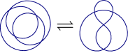
(b) $\displaystyle T_{2}$

(c) $\displaystyle C_{1}$

(d) $\displaystyle E_{1}$

Figure 2: Equivalent knot shadow diagrams.

2010 Mathematics Subject Classifications: 05A19; 57M25.