Studying the Milky Way Pulsar Population with Cosmic-Ray Leptons

Abstract

Recent measurements of cosmic-ray electron and positron spectra at energies from a GeV to 5 TeV, as well as radio, X-ray and a wide range of gamma-ray observations of pulsar-wind nebulae, indicate that pulsars are significant sources of high-energy cosmic-ray electrons and positrons. Here we calculate the local cosmic-ray $e^{\pm}$ energy spectra from pulsars taking into account models for (a) the distribution of the pulsars spin-down properties; (b) the cosmic-ray source spectra; and (c) the physics of cosmic-ray propagation. We then use the measured cosmic-ray fluxes from AMS-02, CALET and DAMPE to constrain the space of pulsar and cosmic-ray-propagation models and in particular, local cosmic-ray diffusion and energy losses, the pulsars’ energy-loss time-dependence, and the injected $e^{\pm}$ spectra. We find that the lower estimates for the local $e^{\pm}$ energy losses are inconsistent with the data. We also find that pulsar braking indexes of 2.5 or less for sources with ages more than 10 kyr are strongly disfavored. Moreover, the cosmic-ray data are consistent with a wide range of assumptions on the $e^{\pm}$ injection spectral properties and on the distribution of initial spin-down powers. Above a TeV in energy, we find that pulsars can easily explain the observed change in the $e^{+}+e^{-}$ spectral slope. These conclusions are valid as long as pulsars contribute $\gtrsim 10\%$ of the observed cosmic-ray $e^{\pm}$ at energies $\gtrsim 100$ GeV.

I Introduction

Observations of of electromagnetic radiation from pulsars and their surrounding environment, including the pulsar wind nebulae (PWNe), from radio wavelengths to $\gamma$-rays Kuiper et al. (2001, 2004); Thompson (2004); Gaensler and Slane (2006) suggest that pulsars are a significant source of high-energy cosmic-ray electrons and positrons. In particular, HAWC Abeysekara et al. (2017a, b) and Milagro Abdo et al. (2009) both recently observed $\gamma$-ray halos at energies of 10 TeV and above around Geminga and Monogem, two nearby pulsars. These observations are well accounted for by the escape of cosmic-ray $e^{\pm}$ from the relevant PWNe which then produce the observed gamma-rays via inverse-Compton scattering (ICS) of background light within a volume of $\sim 10^{3}$ pc³ around the pulsar Hooper et al. (2017); Abeysekara et al. (2017b). Follow-up observations will soon address remaining uncertainties in the diffusion and energy losses of these leptons in the interstellar medium (ISM) and the possible effects of convective winds around Geminga and Monogem. Still, current data already indicate that pulsars and PWNe can accelerate significant fluxes of $e^{\pm}$ with potential implications for future pulsar searches Linden et al. (2017).

Cosmic-ray electrons are also thought to be shock-accelerated to energies between a keV and $\sim 100$ TeV in supernova remnants. At low energies, cosmic-ray electrons and positrons may also be produced from inelastic collisions of cosmic-ray nuclei with nuclei in the ISM. These are commonly known as secondary electrons and positrons, and numerical codes calculating their spectra have been developed e.g., in Refs. Moskalenko et al. (2002); Kachelriess et al. (2015); http://galprop.stanford.edu/. ; Carmelo et al. (2008); http://dragon.hepforge.org .

There is roughly one pulsar born in the Galaxy per century Dragicevich et al. (1999); Vranesevic et al. (2004); Faucher-Giguere and Kaspi (2006); Lorimer et al. (2006); Keane and Kramer (2008). Electrons and positrons suffer from energy losses due to synchrotron radiation and ICS off the cosmic microwave background (CMB) and infrared/optical starlight as they diffusively propagate through the ISM. The interplay of diffusion and energy losses gives a rough maximum energy $E_{\rm max}\sim 100\,{\rm GeV}(R/2\,{\rm kpc})^{-2}$ Cholis et al. (2018) for $e^{\pm}$ that survive at a distance $R$ from their source. Thus, fewer sources can contribute to the $e^{\pm}$ flux observed at higher energies at any given location. A rate of one pulsar per century suggests that only a few dozen pulsars contribute to the $e^{\pm}$ flux above 500 GeV. The discreteness of the source population can result in spectral features in the $e^{\pm}$ energy spectra Malyshev et al. (2009); Grasso et al. (2009) that might be sought, e.g., with a fluctuation analysis of the energy spectra Cholis et al. (2018).

The aim of this paper is to use existing measurements of the $e^{\pm}$ energy spectra to constrain the properties of the pulsar population within a few kpc from the Earth. We do so by simulating a large number of realizations of pulsar distributions for an array of models of the astrophysical conditions impacting the cosmic-ray spectra from pulsars. We first simulate the spatial distribution of pulsars. Then for each simulation, we calculate the local CR $e^{\pm}$ spectrum for an array of different assumptions on the injected $e^{\pm}$ spectra and cosmic-ray propagation conditions. By requiring the local cosmic-ray $e^{\pm}$ energy spectra to agree with measurements, we exclude over three quarters of the models and find several conclusions that can be drawn even after marginalizing over the model uncertainties. These conclusions include that braking indexes of 2.5 or less, that have been observed for some very young pulsars, are excluded by CR data that rely on the characteristics of sources older than 10 kyr. Furthermore, we show that if the local ISM conditions result in low energy losses, then pulsars can not explain the data. If such conditions are avoided, pulsars can explain the CR data with the positron fraction above 300 GeV being either flat, increasing or decreasing with energy. Additionally, a total $e^{+}+e^{-}$ spectrum with a softer slope is a typical expectation of pulsar sources if very young sources such as Vela are still subdominant contributors in the local $e^{\pm}$.

This paper is organized as follows: In Section II we describe the simulations, enumerate the assumptions made, and clarify the astrophysical uncertainties involved in the simulations. In Section III we present the simulations that are allowed by the data. We discuss first our fits to the AMS-02 positron fraction ($e^{+}/(e^{+}+e^{-})$) measurement. Then we show the impact of adding into our analysis $e^{+}+e^{-}$ fluxes from CALET and DAMPE. We conclude and discuss future directions in Section IV.

II Method

II.1 Cosmic Ray Data

We use the published AMS-02 data from Ref. Accardo et al. (2014) collected over a period of 2.5 years. We ignore the measurement associated with energies below 5 GeV since at these energies the spectra are strongly affected by the solar wind and because pulsars contribute marginally. We focus instead on the measurement above 5 GeV and up to 500 GeV. In addition, we consider the impact of a turnover in the positron fraction above 500 GeV, as suggested recently Collaboration (2018). Since this is not a published measurement, we indicate the impact if the result stands, but also provide results without it. In addition, we use the 1.5 years of spectral measurements of the combined $e^{+}+e^{-}$ CR flux, from 25 GeV up to 5 TeV, by DAMPE Chang et al. (2017); Ambrosi et al. (2017) as well as the same spectral measurements by CALET Adriani et al. (2015, 2017, 2018) at energies between 10 GeV and 5 TeV, taken over an extension of two years. We note that the measurements by DAMPE and CALET are in statistical tension with each other and thus avoid fiting to both data sets. Instead, we only check for consistency between the AMS-02 positron fraction and each of these electron- plus-positron spectra separately.

II.2 Studying the Pulsar Population

The contribution of local pulsars to the measured CR spectra is influenced by uncertainties. We model these uncertainties by producing astrophysical realizations spanning the relevant multi-dimensional parameter space in a discrete manner. We call these unique points on this space pulsar astrophysical realizations or just simulations. An example of four such pulsar astrophysical realizations is shown in Fig. 1. The current data show that the positron fraction rises monotonically from 7 GeV to $\sim$300 GeV. We show several simulations that fit the data over the range that it is measured. These fitted simulations show that the spectrum can either continue to rise to a value $\mathrel{\raise 1.29167pt\hbox{$>$\kern-7.5pt\lower 4.30554pt\hbox{$\sim$}}}0.20$ at an energy of a TeV or flatten to a value of $\simeq 0.16$, or even drop to $\simeq 0.1$ at that energy. AMS-02 will have the sensitivity to eventually observe such values of the positron fraction. Moreover, different astrophysical realizations can predict a pulsar spectrum that is inherently smooth and featureless or one that has detectable features Cholis et al. (2018).

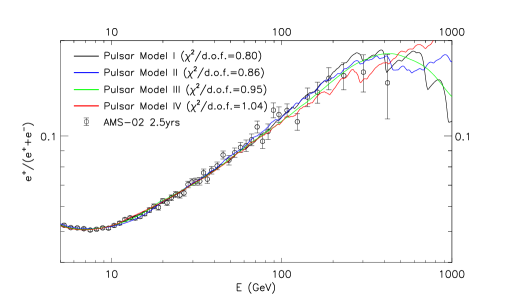
Figure 1: Four different pulsar astrophysical realizations. The predicted positron-fraction spectrum, which is observed to increase from 7 to $\sim$300 GeV, can either drop at higher energies (model I, in black line), flatten out (model II, in blue line), or keep rising up to a TeV (model IV, in red line). Also depending on the exact ISM assumptions (see text for details and Fig. 3), it can be smooth (green line) or have features associated with individual pulsars whose presence can potentially be detected Cholis et al. (2018).

II.2.1 Neutron star birth distribution

As discussed in the Introduction, the cosmic-ray $e^{\pm}$ observed locally come from sources within a radius $R$ from us where, as described in the Introduction, that radius is smaller at higher energies. Thus, the observed cosmic-ray $e^{\pm}$ flux is sensitive to the spatial distribution and birth rate within this volume. The birth rate and spatial distribution of pulsars within the Milky have been subjects of extensive work Lorimer (2003); Lorimer et al. (2006); Faucher-Giguere and Kaspi (2006); Yusifov and Kucuk (2004). Yet there are great uncertainties in both, given the lack of a complete pulsar survey of the sky at radio wavelengths. Moreover, the pulsars’ radio emission is highly anisotropic, beamed with an opening angle spanning about one tenth of the pulsars’ $4\pi$ steradians. In fact, observations suggest that this ratio (typically referred to as the beaming fraction) is time-dependent, being larger at the earlier stages of the pulsar’s evolution (as high as $\simeq 50\%$ during its first 10 kyr) and gradually decreasing Tauris and Manchester (1998). At gamma-ray wavelengths, the surveys do span the entirety of the sky but are sensitive only to the brightest sources, i.e., the most powerful, younger, and nearby members of the pulsar population.

The Milky Way pulsar birth rate has been estimated to be $1.4\pm 0.2$ per century in Ref. Lorimer et al. (2006), with alternative estimates that range between one and four per century at one $\sigma$ Vranesevic et al. (2004); Faucher-Giguere and Kaspi (2006); Keane and Kramer (2008) and even as high as $\simeq 8$ per century Dragicevich et al. (1999). In our analysis, the pulsar birth rate is degenerate with the fraction of spin-down power that goes to high energy $e^{\pm}$ and thus for simplicity we choose it to be one per century. The spatial distribution of pulsars at birth is expected to follow the stellar distribution in the Milky Way’s spiral arms. It has been modeled in Refs. Faucher-Giguere and Kaspi (2006); Lorimer (2003); Lorimer et al. (2006) based on the Parkes multi-beam survey at 1.4 GHz Manchester et al. (2001). We generate simulations of Milky Way pulsar populations. To generate simulations of Milky Way pulsar populations, we follow both the parametrization of Ref. Lorimer (2003) and Ref. Lorimer et al. (2006) taking the latter as the canonical distribution. More precisely, for the distribution of pulsars in galactocentric distance $r$ we use the radial density profile,

$$\rho(r;B,C)=A\left(\frac{r}{R_{\odot}}\right)^{B}\exp\left(-C\left[\frac{r-R_{\odot}}{R_{\odot}}\right]\right),$$ (1)

where $B=1.9$, $C=5.0$, $R_{\odot}=8.5$ kpc, and $A$ is normalized to a pulsar birth rate of one per century. Furthermore, in our generated simulations, pulsars have a distance $z$ away from the disk that follows a Laplace distribution with a scale height of 50 pc and mean of 0 pc, in accordance with Ref. Faucher-Giguere and Kaspi (2006). Finally, we do not try to simulate the spiral arms of the Galaxy, but simply assume a uniform distribution in Galactocentric angle.

II.2.2 Neutron-Star spin-down

Neutron stars (NSs) are born from the core collapse of massive stars in the range of 8–25 $M_{\odot}$. Given their violent birth combined with supernova explosions not being perfectly spherically symmetric, neutron stars have large three-dimensional kick velocities (e.g. Ref. Hobbs et al. (2005) find kick velocity to be $400\pm 40$km/s) and also large ($\sim 10^{49}$ erg) initial rotational energies. They also have strong magnetic fields due to the contraction of the initial core, with large uncertainties in the magnetic-field strengths due to magnetohydrodynamic instabilities formed in the early stages of the NS birth. The strength of the initial magnetic fields at the poles ranges between $\sim 10^{12}-10^{15}$ G. These rapidly rotating strong magnets will suffer the loss of rotational energy with initial spin-down powers that may also span orders of magnitude given the large uncertainties in the initial magnetic fields and rotational frequencies. This spin-down power evolves with time as,

$$\dot{E}(t)=\dot{E_{0}}\left(1+\frac{t}{\tau_{0}}\right)^{-\frac{\kappa+1}{\kappa-1}}.$$ (2)

Here, $E_{0}$ is the initial rotational energy (i.e. $E_{0}=1/2\;I_{0}\Omega_{0}^{2}$, with $I_{0}$ the neutron-star moment of inertia and $\Omega_{0}$ its initial angular frequency),

$$\tau_{0}=\frac{\dot{\Omega}}{(\kappa-1)\Omega}\left[1-\left(\frac{\Omega}{\Omega_{0}}\right)^{\kappa-1}\right]$$ (3)

is the characteristic timescale, or age, of a pulsar, and $\kappa$ is the braking index describing the time evolution of the neutron stars’ angular frequency $\Omega$ through $\dot{\Omega}\propto\Omega^{\kappa}$. Setting $\kappa=3$ describes the spin-down due to magnetic-dipole radiation Manchester and Taylor (1977). Measurement of $\kappa$ demands knowledge of $\Omega$, $\dot{\Omega}$ and $\ddot{\Omega}$ ($\kappa\equiv\ddot{\Omega}\Omega/\dot{\Omega}^{2}$). This biases the measurement toward young pulsars where $\ddot{\Omega}$ is not too small to measure, and young pulsars may not be characteristic of the general distribution. Typical observed values give $\kappa\mathrel{\raise 1.29167pt\hbox{$<$\kern-7.5pt\lower 4.30554pt\hbox{$\sim$}}}3$ Lyne et al. (1993); Gouiffes et al. (1992); Livingstone et al. (2005a); Lyne et al. (1996); Camilo et al. (2000); Kaspi et al. (1994); Livingstone et al. (2005b); Espinoza et al. (2017); Marshall et al. (2016), but there are also recent measurements of young pulsars with higher braking-index values Archibald et al. (2016). Moreover the pulsar braking index may evolve with time Manchester and Taylor (1977); Tauris and Manchester (1998) depending on the specific properties of the pulsar Johnston and Karastergiou (2017).

Given these uncertainties, our simulations test three different choices, $\kappa=2.5$, 3.0, and 3.5 for the braking-index. For each choice, we also choose a value for the characteristic spin-down timescale $\tau_{0}$. Finally, we account for pulsars not having a universal initial spin-down power given the wide ranges of observed magnetic fields for young pulsars ($\sim 10^{12}-10^{14.5}$ G). We simulate pulsars with an initial spin-down power $\dot{E_{0}}$ given by

$$\dot{E}_{0} = 10^{x}\textrm{ erg/s}=10^{x_{\textrm{cutoff}}-y}\textrm{ erg/s},\textrm{ with}$$

$$f(y) = \frac{\textrm{Exp}\left\{-\frac{[-\mu_{y}+ln(y)]^{2}}{2\sigma_{y}^{2}}\right\}}{\sqrt{2\pi}y\sigma_{y}}.$$ (4)

The values for $x_{\textrm{cutoff}}$ and $\mu_{y}$ are constrained by radio observations of rotation periods and modeled surface magnetic fields of Myr old pulsars Faucher-Giguere and Kaspi (2006). Moreover observation of the Crab pulsar at $\simeq 1$ kyr imposes a hard cut-off on observed spin-down power of pulsars larger than $10^{38.7}$ erg/s Manchester et al. (2005); http://www.atnf.csiro.au/research/pulsar/psrcat . In our simulations we take $\sigma_{y}=[0.25,0.36,0.5,0.75]$. Those observational constraints result in pulsars with $\tau_{0}$ values as small as 0.6 kyr for $\kappa=2.5$ and as large as 30 kyr for $\kappa=3.5$, with typical values of 6–10 kyr for breaking index of 3.0. In Fig. 2, we show normalized histograms of $\dot{E}$ for each value of $\sigma_{y}$ for simulations that are allowed by the data.

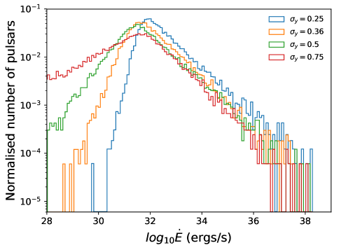
Figure 2: Shown here are normalized histograms of pulsar luminosities from various realizations. This is not their birth luminosity, but the luminosity evolved to today using Eq. 2. All simulations shown have a braking index of $\kappa=3.0$. The surface magnetic fields as well as periods of pulsars with distributions in orange and red are in good agreement with results shown in Fig. 6 of Ref. Faucher-Giguere and Kaspi (2006). For the blue histogram, the surface magnetic fields of simulated pulsars and for the green, their periods agree well with Ref. Faucher-Giguere and Kaspi (2006). At high luminosities one can notice the Poisson fluctuations that arise in each individual simulation. All distributions shown are associated with models that are allowed by the data.

We allow for a wide range of assumptions regarding the true underlying current period of pulsars with ages $\leq 10$ Myr, as well as their surface magnetic fields. Since we rely on observations of pulsars with ages of order $10^{5}$-$10^{7}$ years, we probe predominantly that population and not the spin-down conditions in the very early stages. We then use the CR measurements to constrain the birth properties of the pulsar population.

We also note that neutron-star kick velocities of $\sim 100$ km/s result in a displacement of $\sim 100$ pc of the NSs from their birth location within 1 Myr, but only a few pc in their first $\sim$10 kyr ($\simeq\tau_{0}$) that is relevant for our work. We thus take their distribution in space to be their distribution at birth.

II.2.3 Injection properties of cosmic-ray $e^{\pm}$

From radio and microwave observations of synchrotron radiation close to the NS magnetic poles and of inverse Compton scattering in gamma rays further away from the NS, we know that $e^{\pm}$ pairs are produced and get accelerated inside the pulsar magnetospheres (up to distance scales $O(10^{4}-10^{5})$ km) Rees and Gunn (1974); Arons and Schrlemann (1979); Cheng et al. (1986); Daugherty and Harding (1996); Contopoulos et al. (1999); Komissarov (2006); Gruzinov (2005); Contopoulos and Spitkovsky (2006); Spitkovsky (2006); Harding et al. (2008); Kalapotharakos and Contopoulos (2009); Watters et al. (2009); Bai and Spitkovsky (2010); Bühler and Blandford (2014); Cerutti et al. (2015). In addition, $e^{\pm}$ can get accelerated outside the pulsar magnetosphere before or at the PWN termination shock that typically extends out to $\sim$pc distances from the NS Goldreich and Julian (1969); Hoshino et al. (1992); Lyubarsky and Kirk (2001); Lyubarsky (2003); Sironi and Spitkovsky (2011); Bühler and Blandford (2014); Sironi and Spitkovsky (2014); Zenitani and Hoshino (2001); Kargaltsev et al. (2015). In fact, there is evidence for the presence of $\sim 100$ TeV $e^{\pm}$ at even larger distances, of $\simeq 10$ pc, from HAWC observations of gamma rays at $\sim 10$ TeV from the pulsars Geminga and Monogem Abeysekara et al. (2017a, b). All these observations suggest that pulsars are environments that are rich in high-energy $e^{\pm}$, a fraction of which may escape into the ISM as cosmic rays.

Following Ref. Malyshev et al. (2009), we assume that each pulsar is a point source of CR $e^{\pm}$ described by a source term,

$$Q(E,\vec{x},t) = \frac{dN}{dE}\delta(\vec{x})\left(1+\frac{t}{\tau_{0}}\right)^{-\frac{\kappa+1}{\kappa-1}},\;\textrm{with}$$

$$\frac{dN}{dE} = Q_{0}\big{(}\frac{E}{1\textrm{GeV}}\big{)}^{-n}Exp\{-\frac{E}{E_{\textrm{cut}}}\},$$ (5)

the CR energy density from a given pulsar. Here, $\delta(\vec{x})$ is a Dirac delta function localized at the pulsar position, and the normalization of $Q_{0}$ is such that Malyshev et al. (2009),

$$\int\int\int dE\,d\vec{x}\,dt\,Q(E,\vec{x},t)=\eta W_{0},$$ (6)

where $\eta$ is the fraction of the rotational energy $W_{0}$ that has already been lost through CR $e^{\pm}$ injected into the ISM. This gives,

$$Q_{0}=\frac{E_{\textrm{cut}}^{2-n}}{\Gamma(2-n)}\,\frac{2}{(\kappa-1)\tau_{0}},$$ (7)

where $\Gamma(2-n)$ is the Euler gamma-function, $n<2$, and $\kappa>1$. The total amount of available rotational energy depends on the exact initial spin-down power and its time evolution. We use Eq. 2, which for $t\gg\tau_{0}$, gives $W_{0}=\dot{E_{0}}\tau_{0}$, while for $t\sim\tau_{0}$, there is a correction factor of $(1+t/\tau_{0})^{(\kappa+1)/(\kappa-1)}$.

We are agnostic on the exact values of $\eta$ and $n$ of each pulsar, but X-ray and $\gamma$-ray observations suggest values of $n\simeq 1.4-2.0$ Bietenholz et al. (1997); Halpern and Ruderman (1993); Fierro et al. (1998); Thompson (1999); Atoyan (1999); Kuiper et al. (2001); Abdo et al. (2010a, b, 2013), even though observations of gamma rays from the Crab pulsar reveal a significantly softer spectrum for the high-energy CR $e^{\pm}$Fierro et al. (1998); Abdo et al. (2010a). There are thus significant observed source-to-source variations among pulsars, especially at higher energies. In our simulations, we do not assume that all pulsars have the same values of CR $e^{\pm}$ injection indexes and spin-down power efficiencies (to CRs). Instead, the parameter $n$ follows a uniform distribution $g(n)$. We use two different assumptions for $g(n)$ in assigning an injection index $n$ to each pulsar of a given simulation; they are

$$n\epsilon\begin{cases}[1.6,1.7],\,\,\,\,\,\,\,\textrm{option "a"}\\ [1.4,1.9],\,\,\,\,\,\,\,\textrm{option "b"}.\end{cases}$$ (8)

Similarly, each pulsar in a given simulation has a value of $\eta$ taken from a log-normal distribution Cholis et al. (2018),

$$h(\eta)=\frac{Exp\left\{-\frac{\left[-\mu+ln(-1+\eta)\right]^{2}}{2\sigma^{2}}\right\}}{\sqrt{2\pi}(\eta-1)\sigma}.$$ (9)

We do not know what the exact range of the $\eta$ values should be. We therefore have in our simulations three options in choosing values for $\mu$ and $\sigma$ in Eq. 9. The more physically intuitive quantities are the mean efficiency $\bar{\eta}=1+\textrm{Exp}\left\{\mu+\frac{\sigma^{2}}{2}\right\}$ and the parameter $\zeta=10^{\sqrt{\sigma}}$. For a given produced simulation, $\zeta$ is fixed but $\bar{\eta}$ is normalized to the CR data. The three choices for log-normal distributions $h(\eta)$ are

$$(\bar{\eta},\zeta)=\begin{cases}(2\times 10^{-2},1.29),\,\,\,\,\,\,\,\textrm{option "a"}\\ (4\times 10^{-3},1.47),\,\,\,\,\,\,\,\textrm{option "b"}\\ (1\times 10^{-3},2.85),\,\,\,\,\,\,\,\textrm{option "c"},\end{cases}$$ (10)

where the $\bar{\eta}$ values refer to the starting point before the fit. Typically, the values of $\bar{\eta}$ do not change by more than a factor of a few, with large values of $\zeta$ leading to smaller values of $\bar{\eta}$.

We note that the exact assumption for the value of the injection upper cutoff $E_{\textrm{cut}}$ does not affect our results as $e^{\pm}$ that propagate into the ISM cool down very rapidly. We take $E_{\textrm{cut}}=10$ TeV.

II.2.4 Propagation of Cosmic rays

Cosmic rays injected into the ISM by individual pulsars have to travel from their simulated locations in the Milky Way to the Earth’s location where they are detected by the AMS-02, DAMPE, and CALET instruments. They propagate first through the ISM before entering the volume affected by the solar magnetic field and wind. During that first propagation, the $e^{\pm}$ diffuse through the complicated galactic magnetic-field structure and lose energy via synchrotron radiation as well as ICS with the CMB and ambient infrared and optical photons. The first process is described by the diffusion coefficient,

$$D(E)=D_{0}(E/1\textrm{GeV)}^{\delta},$$ (11)

assumed for simplicity to be homogeneous and isotropic within a thick several-kpc diffusion disc around the Milky Way stellar disc, where the pulsars reside. The energy losses are described by

$$dE/dt=-b\,E^{2},$$ (12)

where $b$ is proportional to the sum of the energy densities of the local (within a few kpc) magnetic field $U_{\textrm{B}}$ and the local radiation field $U_{\textrm{rad}}$. Relying on previous studies of the CR boron-to-carbon (B/C) ratio observed by both PAMELA and AMS-02 and also on the CR proton data observed by PAMELA and Voyager 1, Malyshev et al. (2009); Trotta et al. (2011); Cholis et al. (2016) we adopt five different ISM models for the CR propagation in our analysis. These are described in Table 1.

Model	$b$ ($\times 10^{-6}$GeV-1kyr-1)	$D_{0}$ (pc2/kyr)	$\delta$
A1	5.05	123.4	0.33
C1	5.05	92.1	0.40
C2	8.02	92.1	0.40
C3	2.97	92.1	0.40
E1	5.05	58.9	0.50

Table 1: The parameters for each of our five ISM propagation models; see Eqs 11, 12 and text for details.

After their ISM propagation and before their detection, CRs travel through the time-evolving solar wind. For energies $E\leq 10$ GeV, the effect on the CR spectra is known as solar modulation. This is the imprint of the diffusion, drift, and adiabatic energy losses experienced by CRs traveling through the complex magnetic field structure of the heliosphere (within $\simeq$100 au from the Sun). This solar modulation is described by imposing a translation in the energy of the CR spectra as Gleeson and Axford (1968),

$$\frac{dN^{\oplus}}{dE_{\textrm{kin}}}(E_{\textrm{kin}}) = \frac{(E_{\textrm{kin}}+m)^{2}-m^{2}}{(E_{\textrm{kin}}+m+|Z|e\Phi)^{2}-m^{2}}$$ (13)

$$\times \;\frac{dN^{\rm ISM}}{dE_{\textrm{kin}}}(E_{\textrm{kin}}+|Z|e\Phi).$$

Here, $E_{\textrm{kin}}$ is the observed kinetic CR energy at Earth ($\oplus$), while $\frac{dN^{\oplus(\textrm{ISM})}}{dE_{\textrm{kin}}}$ the differential CR flux at Earth. The equivalent $E_{\textrm{kin}}$ for the ISM spectrum is (on average) $E_{\textrm{kin}}+|Z|e\Phi$, where $\Phi$ is the modulation potential. Finally, $|Z|e$ is the absolute value of the CR charge.

Ref. Cholis et al. (2016) used archival data to obtain a time-, charge- and rigidity(R)-dependent formula

$$\Phi(R,q,t)= \phi_{0} \,\bigg{(}\frac{|B_{\rm tot}(t)|}{4\,{\rm nT}}\bigg{)}+\phi_{1}\,H(-qA(t))\,\bigg{(}\frac{|B_{\rm tot}(t)|}{4\,{\rm nT}}\bigg{)}$$ (14)

$$\times \,\bigg{(}\frac{1+(R/R_{0})^{2}}{\beta(R/R_{0})^{3}}\bigg{)}\,\bigg{(}\frac{\alpha(t)}{\pi/2}\bigg{)}^{4}$$

for the solar modulation potential. Following that work, $R_{0}$ is set to 0.5 GV. Instead $\phi_{0}$ and $\phi_{1}$ are marginalized within $[0.32,0.38]$ GV and $[0,16]$ GV respectively. The values for $B_{\textrm{tot}}(t)$ and $\alpha(t)$ are averaged over 6-month periods using the measurement by the ACE satellite http://www.srl.caltech.edu/ACE/ASC/ and the models of the Wilcox Solar Observatory http://wso.stanford.edu/Tilts.html . The potential $\Phi(R,q,t)$ is time dependent for every species, different between electrons and positrons observed at the same time and rigidity, and is smaller for larger rigidities becoming $\Phi(R,q,t)\rightarrow\phi_{0}(|B_{\textrm{tot}}(t)|)/(4\,\textrm{nT})$.

II.2.5 Combining all the pulsar-population uncertainties

To combine all the astrophysical uncertainties, we first generate a pulsar population in the Milky Way with an assumed spatial distribution and birth rate, and a given choice of $\kappa$, $\tau_{0}$, and $f(y)$ characterizing the initial spin-down power and its evolution. There are 30 different combinations of these assumptions (see Appendix A of Cholis et al. (2018) for details). These pulsars also follow the distributions $g(n)$ and $h(\eta)$ on the injection properties. There are six combinations for these two distributions, which we refer to as "aa", "ba", "ab", "bb", "ac", and "bc", where the first letter refers to the $g(n)$ options "a" or "b" of Eq. 8 and the second letter to $h(\eta)$, with its options "a-c" of Eq. 10. We also choose one of the five ISM propagation models described by Table 1, while we marginalize over parameters $\phi_{0}$ and $\phi_{1}$ of Eq. 14 to account for solar modulation. Those choices result in $30\times 6\times 5=900$ different astrophysical realizations/simulations that we test.

Each one of these astrophysical realizations is fitted to the CR data by allowing for five fitting parameters, $\phi_{0}$, $\phi_{1}$, the normalization of the primary CR electron flux, the normalization of the secondary CR $e^{\pm}$ fluxes and the normalization of the total pulsar CR $e^{\pm}$ fluxes at the location of the Sun (outside the heliosphere). The impact of these different astrophysical choices on the positron fraction spectrum is given in Fig. 3. The five different colored lines refer to the five ISM models.

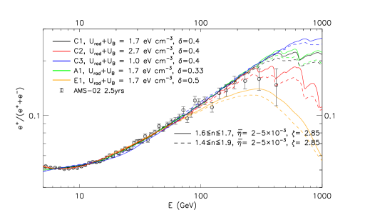
Figure 3: The effects of changing assumptions in our astrophysical pulsars realizations. Top: Different color lines depict the effect that changing only the CR propagation through the ISM, (i.e. CR diffusion and energy-losses described by Eqs. 11 and 12) has on the expected flux from what is otherwise the same simulation of pulsar sources in the Milky Way. ISM Models "C1", "C2", "C3", "A1" and "E1" are described in Table 1. As described in the main text, we fit the simulations to the AMS-02 data. The solid vs dashed lines for every given colored line show the impact on our results of changing solely the distribution of the CR injection indexes $g(n)$ (see Eq. 8 and also Eq. 5). Bottom: For a specific assumption on the ISM propagation conditions ("C2"), we show in the six types of lines, the effect of varying the assumptions on $g(n)$ and $h(\eta)$ (see Eqs 5, 8 and 9, 10 respectively and discussion therein).

In the top panel of Fig. 3 and for the choice "c" of $h(\eta)$, we give the two choices for $g(n)$; i.e., the choices "ac" and "bc" in solid and dashed lines respectively. Different ISM assumptions can enhance ("A1", "C2" choices) or suppress ("C3", "E1" choices) the small-scale (in energy range) features of the spectra. At high energies when the energy-loss rate is assumed to be larger (smaller) or the CR diffusion slower (faster), the small-scale spectral features are more (less) pronounced. Similarly, when a wider range of injection indexes $n$ is assumed, the resulting features are more evident (from the fact that Poisson fluctuations of nearby sources with hard injected spectra being dominant are more common). Moreover, since the fits are dominated by the low-energy data, different ISM models can predict significant variations at high energies. For instance, "A1" models faster diffusion of low-energy CRs, but with a smaller diffusion index $\delta=0.33$, which in turn increases the escape timescale of CRs from the Galaxy, and thus enhancing their flux at high energies. Model "E1" represents the reverse assumption (slow diffusion of low-energy CRs but with a larger diffusion index $\delta=0.5$ leading to faster escape at high energies) suppressing the high-energy fluxes. Model "C1" represents a more intermediate case. Also, larger/smaller energy losses (modeled by "C2"/"C3") suppress/enhance the high-energy CR pulsar fluxes.

The bottom panel of Fig. 3 shows, for a fixed choice ("C2") of ISM assumptions, the impact of varying the $g(n)$ and $h(\eta)$ choices. A wider range of the $\zeta$ parameter, associated with the standard deviation in the $h(\eta)$, results in more pronounced features. We also note that when $\zeta$ is larger, a few pulsars may deposit a larger fraction of their spin-down power to CR $e^{\pm}$ in the ISM. In turn, the fits are forced to compensate for that by reducing the averaged $\bar{\eta}$ value.

III Results

III.1 Using only the AMS-02 positron fraction data

Our fits to the AMS-02 positron-fraction spectrum allow us to constrain combinations of the above mentioned astrophysical uncertainties via data not previously used to probe the pulsar population properties of the Milky Way. Of the 900 astrophysical realizations, only 205(160) can fit the positron fraction spectrum within 3$\sigma(2\sigma$) from an expectation of $\chi^{2}$ of 1 for each degree of freedom These astrophysical realizations are depicted in Fig. 4.

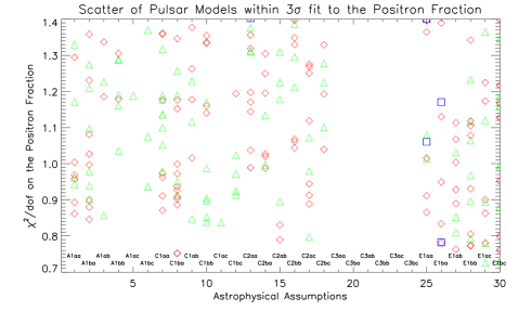
Figure 4: The scatter of astrophysical pulsar realizations that fall within our 3$\sigma$ constraint to the AMS-02 positron fraction data. On the y-axis we give the $\chi^{2}$/d.o.f. value, while on the x-axis we give the astrophysical assumptions, e.g. "A1aa" refers to ISM model "A1" and $g(n)$ and $h(\eta)$ distributions choice "aa" of Eqs. 8 and 10 respectively. Blue boxes are for braking index $\kappa$ of 2.5, red diamonds for $\kappa=3.0$ and green triangles for $\kappa=3.5$. Two evident results are that i) very few pulsar population realizations with $\kappa=2.5$ survive the positron fraction fit and ii) there are no realizations with ISM conditions "C3" allowed by the data (see text for further details).

In Fig. 4, the y-axis gives the $\chi^{2}$ per degree of freedom for the positron fraction data. The x-axis represents the probed parameter space in 30 distinct combinations of assumptions. These mark the assumptions on the CR $e^{\pm}$ ISM propagation described by the first two characters ("A1", "C1", "C2", "C3", "E1") as well as the CR injection properties both with regards to the injection index $n$-distribution $g(n)$ of Eq. 8 and the $h(\eta)$ distribution of Eq. 10. The latter assumptions are depicted by the last two characters ("aa", "ba", "ab", "bb", "ac", "bc"). For example the first discrete point in the x-axis ("A1aa") refers to ISM model "A1" of Table 1 while the third character "a" stands for $n\epsilon[1.6,1.7]$ and the last character for $(\bar{\eta},\zeta)=(2\times 10^{-2},1.29)$ (case "a"). Each allowed pulsar population simulation is represented by a shape. Blue boxes are for $\kappa=2.5$, red diamonds are for $\kappa=3.0$ and green triangles for $\kappa=3.5$.

From our fits to the positron fraction, we have two major findings. The first is that while we run 240 realizations with a braking index of $\kappa=2.5$, only 5(3) survive within the 3(2) $\sigma$ fit threshold. While there are constraints from radio observations on the period and NS surface B-field, we try to adopt as wide as possible assumptions on the initial spin-down properties of the pulsar populations. These wide assumptions have a significant impact also on the observed pulsar populations as we show in Fig. 2. For the braking index value of 2.5 assumed in the 240 simulations, values for $\tau_{0}$ are in the range of 0.6-1 kyr and of $10^{x_{\textrm{cutoff}}}$ from $10^{38.2}-10^{39}$ erg/s with varying assumptions on $\mu_{y}$ and $\sigma_{y}$ (see Eqs. 2 and 4 and Appendix B of Cholis et al. (2018)). Our second major finding relates to the ISM conditions. For every choice of NS population birth distribution, spin-down properties and pulsars injection of CR $e^{\pm}$ properties, we test each of our five ISM models. Our model "C3" is always excluded as can be seen by the gap in the parameter space in Fig. 4. Table 2 describes the above and provides the fraction of simulations that are allowed by the data (at 3$\sigma$) with the exact number of simulations given in the parentheses.

	A1	C1	C2	C3	E1
$\kappa=2.5$	0 (0)	0 (0)	0.02 (1)	0 (0)	0.08 (4)
$\kappa=3.0$	0.27 (21)	0.40 (31)	0.40 (31)	0 (0)	0.46 (36)
$\kappa=3.5$	0.37 (20)	0.43 (23)	0.35 (19)	0 (0)	0.41 (23)

Table 2: For combinations of the three choices of braking index $\kappa=2.5,3.0,3.5$ and the five choices of ISM propagation conditions "A1", "C1", "C2", "C3", "E1", we give the fraction of pulsar population simulations that are consistent (within our 3$\sigma$ threshold) to the AMS-02 positron fraction spectrum. In the parentheses we give the actual number of the simulations allowed. For the combination of $\kappa=3$ and "A1" we produced 78 simulations to probe the remaining astrophysical parameters, of which 21 (27$\%$) are allowed.

Both sets of assumptions (i.e. $\kappa=2.5$ or ISM model "C3") systematically predict a higher positron fraction than observed above 100 GeV. For the case of the ISM "C3" model, this is straightforward given the suppressed energy-loss coefficient $b$ of Eq. 12. For $\kappa=2.5$, the explanation is as follows. Smaller braking index values demand not only a smaller characteristic timescale $\tau_{0}$, but also result in a faster spinning-down of the pulsars at $t\gg\tau_{0}$, e.g $\dot{E}(t)\propto t^{-2.33}$ for $\kappa=2.5$ vs $\dot{E}(t)\propto t^{-2}$ for $\kappa=3$, (see Eq. 2). In setting the spin-down choices of our pulsar population simulations, we rely on radio observations. These observations probe a wide range of pulsar ages, but there are many more pulsars of age 1-10 Myr than of 10-100 kyr. In our simulations, we check that our pulsar populations are consistent with the late-age properties of the observed pulsars and then effectively evolve backwards in time the pulsars spin-down. Yet, as we explained in section II, most of the pulsars CR flux is produced in the early stages of their evolution. A more abrupt spin-down-power time-evolution as in the $\dot{E}(t)\propto t^{-2.33}$ vs $\propto t^{-2}$ case predicts a higher CR flux overall from each pulsar at a level that is already inconsistent with the CR AMS-02 data. Values of $\kappa<2.5$, as are observed for some of the youngest pulsars, are excluded. Hence, CR data also suggest a time evolution of the braking index.

Moreover, we note that changing the braking index to $\kappa\geq 3$ is enough to exclude the tension with the positron fraction data. Yet as more events are detected from AMS-02 and if indeed a cut-off / drop-off the positron fraction above 500 GeV is confirmed, we will be able to probe/exclude more simulations with $\kappa=3$. The ISM model "A1" that predicts higher CR fluxes due to its diffusion parameters (see Table 1 and Figure 3 top) is currently only mildly less preferred as shown also in Table 2, but we do find that with an observed drop-off of the positron fraction above 500 GeV, many pulsar simulations with the "A1" assumptions can be excluded, while ISM model assumptions "E1" will be slightly preferred ("C1" and "C2" being less affected by the presence of the claimed cut-off).

In addition to the above findings, we note a preference among astrophysical realizations that predict a narrower distribution $h(\eta)$, in the fraction of the spin-down power that goes into CR $e^{\pm}$, with $\zeta$ following hierarchically option "a" ($\zeta\equiv 10^{\sqrt{\sigma}}=1.29$) over option "b" ($\zeta=1.47$) over option "c" ($\zeta=2.85$) as described by Eqs. 9 and 10. This can be seen more directly by our results in Table 3, where we show the slice in parameter space describing the combination of $g(n)$ and $h(\eta)$ injection properties vs the five ISM propagation models. For the narrower $h(\eta)$, anywhere between 23$\%$ and 50$\%$ of our simulations are within our threshold of fit to the positron fraction data. For the wider distribution choices, these fractions are reduced with the widest choice (choices "ac" and "bc") having anywhere between 7$\%$ to 43$\%$ of the simulations within our 3$\sigma$ fitting threshold.

		A1	C1	C2	C3	E1
aa	$1.6\leq n\leq 1.7$, $\eta=2\times 10^{-2}$, $\zeta=1.29$	0.37 (11)	0.43 (13)	0.36 (11)	0 (0)	0.33 (10)
ba	$1.4\leq n\leq 1.9$, $\eta=2\times 10^{-2}$, $\zeta=1.29$	0.46 (14)	0.50 (15)	0.27 (8)	0 (0)	0.23 (7)
ab	$1.6\leq n\leq 1.7$, $\eta=4\times 10^{-3}$, $\zeta=1.47$	0.13 (4)	0.23 (7)	0.27 (8)	0 (0)	0.33 (10)
bb	$1.4\leq n\leq 1.9$, $\eta=4\times 10^{-3}$, $\zeta=1.47$	0.23 (7)	0.36 (11)	0.33 (10)	0 (0)	0.43 (13)
ac	$1.6\leq n\leq 1.7$, $\eta=1\times 10^{-3}$, $\zeta=2.85$	0.07 (2)	0.07 (2)	0.27 (8)	0 (0)	0.33 (10)
bc	$1.4\leq n\leq 1.9$, $\eta=1\times 10^{-3}$, $\zeta=2.85$	0.10 (3)	0.17 (5)	0.20 (6)	0 (0)	0.43 (13)

Table 3: As in Table 2, we present, for the combination of the six choices ("aa", "ba", "ab", "bb", "ac" and "bc") of $g(n)$ and $h(\eta)$ and the five ISM models, the fraction of pulsar simulations that are consistent within 3$\sigma$ with the AMS-02 positron fraction. The numbers in parentheses give the number of the simulations allowed.

We have found no preference towards a narrower or a wider distribution for $\dot{E}_{0}$—i.e., for the parameter $\sigma_{y}$ of Eq. 4.

While still more data from CRs will be necessary, the preference towards a narrow $h(\eta)$ suggests that the pulsar environments do not have very wide source-to-source variations with respect to their output of CR $e^{\pm}$ injected into the ISM.

Finally, we find that there is only a slight preference for the wider $g(n)$ injection index $n$-distribution (option "b" of Eq. 8) over the narrower one (option "a" of Eq. 8). This is evident in the slice of parameter space in Table 4 showing the $g(n)$, $h(\eta)$ parameters versus the braking index $\kappa$.

		$\kappa=2.5$	$\kappa=3.0$	$\kappa=3.5$
aa	$1.6\leq n\leq 1.7$, $\eta=2\times 10^{-2}$, $\zeta=1.29$	0.08 (3)	0.38 (25)	0.36 (16)
ba	$1.4\leq n\leq 1.9$, $\eta=2\times 10^{-2}$, $\zeta=1.29$	0.05 (2)	0.48 (31)	0.27 (12)
ab	$1.6\leq n\leq 1.7$, $\eta=4\times 10^{-3}$, $\zeta=1.47$	0 (0)	0.26 (17)	0.27 (12)
bb	$1.4\leq n\leq 1.9$, $\eta=4\times 10^{-3}$, $\zeta=1.47$	0 (0)	0.32 (21)	0.44 (20)
ac	$1.6\leq n\leq 1.7$, $\eta=1\times 10^{-3}$, $\zeta=2.85$	0 (0)	0.15 (10)	0.22 (10)
bc	$1.4\leq n\leq 1.9$, $\eta=1\times 10^{-3}$, $\zeta=2.85$	0 (0)	0.17 (11)	0.33 (15)

Table 4: Similar to the slices in parameter space given in Tables 2 and 3, we show for the combination of the six choices of $g(n)$ and $h(\eta)$ and the three choices for braking index $\kappa=2.5,3.0,3.5$, the fraction of pulsar population simulations that are consistent within 3$\sigma$ with the AMS-02 positron-fraction spectrum. As before, in the parentheses the actual number of our simulations allowed are given.

We note that more data are being collected by the AMS-02 experiment that can confirm these first indications of preferences in the parameter space of pulsar population properties. In particular, we expect that if a clear cut-off in the positron fraction is observed above 500 GeV in energy, then a significant fraction of the 205 pulsar astrophysical realizations will be excluded.

III.2 Including data from CALET or DAMPE

Recently, two more satellite experiments, CALET Adriani et al. (2015) and DAMPE Chang et al. (2017), have published their measurements of the total $e^{+}+e^{-}$ CR flux up to 5 TeV Adriani et al. (2018); Ambrosi et al. (2017). These spectra allow us to test pulsar-population models at energies where their expected fractional contribution to the total measured quantities can be very significant. For instance at 50 GeV, our fits suggest that the pulsar population is responsible for $\simeq 50\%$ of the measured positron fraction value but only for $\simeq 8\%$ of the observed $e^{+}+e^{-}$ flux. At 500 GeV, pulsars can instead be responsible for as much as $90\%$ of the positron fraction and up to $40\%$ of the $e^{+}+e^{-}$ flux, with the pulsar contribution becoming potentially even more important at higher energies.

III.2.1 The highest energies: understanding the young, nearby pulsars

At higher energies, the combination of volume and age necessary for pulsars to be able to contribute is reduced. Thus the number of sources drops, with the highest energies probing only a small number of pulsars. This should result in $e^{+}+e^{-}$ fluxes rich in features as is shown in Fig. 5, where we compare some of our simulations to the data from CALET (left) and DAMPE (right).

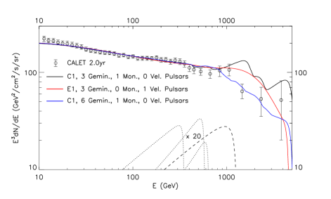
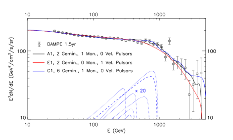
Figure 5: The simulated $e^{+}+e^{-}$ fluxes from combinations of pulsars. We include the primary $e^{-}$ and secondary $e^{\pm}$ CR components. On the left panel we present three simulations that fit well the CALET spectral data depicted, while in the right panel we do the same with the DAMPE spectral data. For the simulations presented we give the number of pulsars that have age, distance from Earth, and current spin-down power in agreement with the observed ones of Geminga ("Gemin"), Monogem ("Mon") and Vela ("Vel") (see text for details). At high energies, we note the presence of several features coming from the contribution of individual pulsars and also a cut-off/change of slope to the total $e^{\pm}$ flux above a TeV due to a small number of contributing sources. We also present for one simulation the fluxes from the individual pulsars that have properties similar to those of Geminga (dotted lines) and Monogem (dashed lines). These fluxes are multiplied by a factor of 20 to lie within the panels’ range. There are large source-to-source variations in our simulations even among Geminga-like pulsars, as we describe in the text.

Additionally at $\simeq 1$ TeV, we find in our simulations that even after smoothing the possible small-scale features, there is typically either a cut-off in the $e^{+}+e^{-}$ flux spectrum or a change in its slope. This is attributed to the fact that only $O(10)$ pulsars can contribute at these energies. The exact energy that this change in the spectrum occurs at and the resulting spectral characteristics depend on these pulsars’ individual properties.

In order to understand the impact of some known nearby pulsars, we compare with similar pulsars in our simulations that fall in our neighborhood. There is extended literature on the possible contribution from Geminga (J0633+1746) and Monogem (B0656+14) to the high-energy positron flux Profumo (2011); Cholis and Hooper (2013); Linden and Profumo (2013); Yin et al. (2013); Linden (2015); Hooper et al. (2017); Abeysekara et al. (2017b); Yuan et al. (2017); Fang et al. (2018). We test the possible contribution from these pulsars by identifying simulations that have pulsars with the same combination of distance from the Earth, age, and current spin-down luminosity as these two pulsars. More specifically, we check for pulsars with (distance, age, $\dot{E}(t=\textrm{age})$) that are within the (distance central value $\pm 1\sigma$, spin-down age${}_{-50\%}^{+100\%}$, spin-down luminosity${}_{-50\%}^{+100\%}$) of the reported (0.25${}_{-0.09}^{+0.45}$ kpc, 3.42$\times 10^{5}$ yr, 3.2$\times 10^{34}$erg/s) for Geminga and (0.29 $\pm$0.15 kpc, 1.11$\times 10^{5}$ yr, 3.8$\times 10^{34}$erg/s) for Monogem Manchester et al. (2005); http://www.atnf.csiro.au/research/pulsar/psrcat . We note that the spin-down age and luminosity rely on the measurements of the period $P$ and its time derivative $\dot{P}$ and are calculated assuming a braking index of $\kappa=3$. Since we want to be agnostic about the true braking index, we allow for the wide range around the central values of age and luminosity. Furthermore, we check for simulations with pulsars that have similar properties as Vela (B0833-45) (0.28 $\pm$ 0.14 kpc, 1.13$\times 10^{4}$ yr, 6.9$\times 10^{36}$erg/s).

In both panels of Fig. 5 we show the CR spectra from three simulations that can explain the data. For each of these simulations the number of pulsars that have distance, age, and luminosity properties similar to Geminga, Monogem, and Vela are provided. It is typically easier to get pulsars like Geminga and Monogem, while a pulsar like Vela is relatively rare. Out of our simulations that fit the positron-fraction data, 75$\%$ have at least one Geminga-like and 18$\%$ at least one Monogem-like pulsar, while only 3$\%$ have at least one Vela-like pulsar.

In each of the Fig. 5 panels, for a chosen simulation, we also plot the predicted $e^{+}+e^{-}$ fluxes from these particular pulsars. Since Vela-like pulsars are younger, their contribution can be dominant only above a few TeV, but the suppression of the total flux suggests that Vela is not a dominant source of $e^{\pm}$ either because these CRs have not yet reached us or because its $\eta$ is suppressed. In fact recent work from Ref. Evoli et al. (2018) suggests that a significant fraction of high energy CRs from very young pulsars (as is Vela) are strongly confined for $O(10)$ kyr before being released into the ISM. Monogem-like pulsars contribute at $\simeq 1$ TeV energies and Geminga-like pulsars at $\simeq 500$ GeV. The exact cut-off energy depends on the ISM energy-losses rate and the individual pulsar’s age. Even after fixing the ISM model and comparing only among the Geminga-like pulsars, there are source-to-source variations in the cut-off due to the age uncertainty that we include for these sources. The amplitude instead depends on their distance from Earth (that in turn has variations since we allow an uncertainty on this as well) and also on the $\eta$ parameter that is unique to each source. Finally the slope for energies lower than the cut-off depends on the diffusion assumptions and on the individual/unique pulsar injection index $n$ (for further details see Ref. Malyshev et al. (2009)).

We note, that we do not over-plot the CALET and DAMPE spectral data and we do not try to fit our simulations simultaneously to both. The measured spectral indexes of the $e^{+}+e^{-}$ flux are in some disagreement between these data-sets, suggesting some energy-scale-related measurement uncertainty.

III.2.2 Combining AMS-02 and CALET data

Instead, we combine the AMS-02 separately with the CALET data. We do that by taking all the original 900 simulations with their best $\chi^{2}$ fit free-parameter values to the positron fraction and test their predicted $e^{+}+e^{-}$ flux to the measurements by CALET and DAMPE respectively. We have noticed that, as is also discussed in Ref. Adriani et al. (2018), the CALET fluxes agree pretty well with the AMS-02 data. For each simulation, in fitting to the CALET (DAMPE) $e^{+}+e^{-}$ data, we allow for an additional $10(20)\%$ freedom in the primary $e^{-}$, secondary $e^{\pm}$ and pulsars $e^{\pm}$ normalizations starting from the best fit values to the positron fraction. Since all the data points are above 10 GeV in energy, the impact of solar modulation is insignificant, and we do not refit the relevant $\phi_{0},\phi_{1}$ parameters.

In Fig. 6 (top panel), we give the scatter of pulsar realizations that are in agreement with the AMS-02 and CALET data within 3$\sigma$ from what is a $\chi^{2}$/d.o.f. of 1. The axes are the same as in Fig. 4 with the exception that the y-axis now refers to the combined data fit. As in Section III.1 we portray the three tested values for the braking index $\kappa$ with there different symbols (boxes, diamonds and triangles for the simulations with $\kappa=2.5$, 3.0 and 3.5). Comparing to the $e^{+}+e^{-}$ flux data, it is easy to acquire a good fit. In fact, of the 205 simulations that are allowed within the 3$\sigma$ threshold by the positron fraction data, 145 are also allowed by the combined positron fraction and $e^{+}+e^{-}$ flux data. As in Fig. 4, those are shown by the blue boxes, red diamonds, and green triangles, respectively. Some pulsar astrophysical realizations have a good enough fit to the CALET data and although not allowed within the 3$\sigma$ threshold by only AMS-02, are allowed by the combined data. There are 14 such simulations in addition to the 145. We show these by magenta diamonds and turquoise triangles for $\kappa=3.0$ and 3.5 respectively, which typically lie on the top end of the y-axis. No additional models with $\kappa=2.5$ were added in the analysis by including the CALET data.

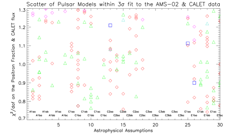
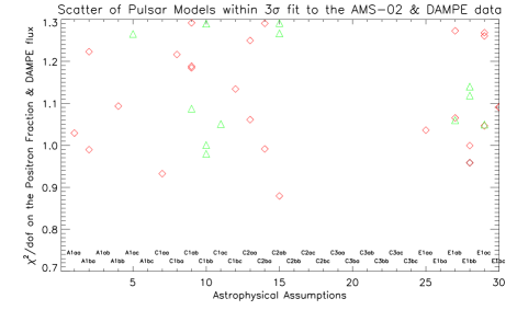
Figure 6: As in Fig. 4, we present the scatter of astrophysical pulsar realizations that fall within our 3$\sigma$ constraint to the combined AMS-02 positron fraction and CALET (top panel) or DAMPE (bottom panel) $e^{+}+e^{-}$ flux data. The y-axis is the $\chi^{2}$/d.o.f. value for the combined data (see text for details), while the x-axis describes the same astrophysical assumptions as in Fig. 4. For each of the three values of braking index that we test, we depict realizations by two colors depending on the quality of their fit to the positron fraction alone. For braking index $\kappa$ of 3.0, the red diamonds are for simulations allowed within 3$\sigma$ by the positron-fraction data. These same simulations are among the 205 simulations described in Section III.1. With magenta diamonds we depict models allowed within 3$\sigma$ by the combined data, but that are excluded by AMS-02 data alone. Similarly, for $\kappa=3.5$, green (turquoise) triangles show the realizations allowed (excluded) by the AMS-02 positron fraction. No additional models with $\kappa=2.5$ are allowed by adding the CALET measurement. With DAMPE data there are no blue, magenta and turquoise symbols.

We find that, as with the positron fraction fit, ISM model "C3" is systematically excluded by the data regardless of the other astrophysical assumptions. In fact, the addition of the flux data does not alter the conclusions of Section III.1 or set further preferences among the remaining ISM models. Similarly, it is still the case that only a small number of simulations with $\kappa=2.5$ (3 out of 159) are allowed, and beyond that, adding the flux data only slightly affects the preference for simulations with $\kappa=3.0$ versus 3.5. Regarding the fraction of the spin-down power going into CR $e^{\pm}$, the preference for narrower $h(\eta)$ is sustained, while the $g(n)$ index of injection distribution properties conclusions are unaffected by the CALET data.

In Figure 7, we also present a histogram of the fitted values of the mean fraction $\bar{\eta}$ of the pulsars population from each realization. The number on the y-axis is the number of these pulsar astrophysical realizations that are allowed. The range of $\bar{\eta}$ to explain the CR data is between $10^{-3}$ and 0.26, with a clear peak at 1–3$\times 10^{-2}$. These fractions assume a Milky Way pulsar birth rate of one per century. If that rate is doubled, those fractions are smaller by the same factor.

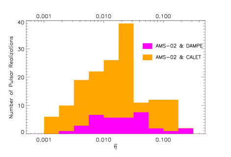
Figure 7: The distribution of the fitted values of the $\bar{\eta}$ parameter for the pulsar-population simulations, allowed within 3$\sigma$ by the combination of AMS-02 $\&$ CALET data (159 astrophysical pulsar realizations in the orange histogram), or allowed by the AMS-02 $\&$ DAMPE data (36 in the magenta histogram).

III.2.3 Combining AMS-02 and DAMPE data

On the other hand, combining the DAMPE $e^{+}+e^{-}$ flux data with the AMS-02 positron fraction dramatically cuts down the parameter space of the pulsar astrophysical realizations allowed (see bottom panel of Fig. 6). Out of the 205 simulations allowed by the positron-fraction data, only 36 remain after combining with DAMPE, while the down-weighting of the AMS-02 data does not lead to any additional simulations allowed within the 3$\sigma$ threshold. We find that none of the $\kappa=2.5$ simulations survive, while 2/3 of these astrophysical realizations are with $\kappa=3$. Regarding the impact of these data on the ISM and $h(\eta)$, $g(n)$ distributions: our results discussed above hold given the small number of remaining simulations. The range of $\bar{\eta}$ is basically the same as that from CALET and AMS-02 data (Fig. 7).

We finally note that tracking the source of the systematic difference between CALET and DAMPE $e^{+}+e^{-}$ data is of great importance in properly combining the data in future analyses.

IV Discussion and Conclusions

We have used CR $e^{\pm}$ data to study the properties of the population of local Milky Way pulsars. Using the AMS-02 positron-fraction measurement and the CALET and DAMPE $e^{+}+e^{-}$ fluxes, we have tested hundreds of pulsars simulations. These simulations probe the astrophysical uncertainties associated with the CR leptonic spectra observed at Earth. In particular, we produce 900 simulations that sample a broad range of possibilities for the spatial distribution of neutron-star birth locations in the Milky Way, for their ages, and their spin-down properties. We also study the effects of uncertainties in the spectra of CR $e^{\pm}$ injected into the ISM and those associated with CR propagation through the ISM. We describe how we model all these astrophysical effects and how we combine them in Section II.

We work under the assumption that pulsars are the dominant source for the rise of the positron fraction at high energies. We find that consistent pulsar-population models can result in a continued rise in the positron fraction with energy, a flattening at energies beyond 300 GeV, or even a drop-off. We also find that consistent models can produce a positron-fraction spectrum that is either smooth in energy or that has fluctuations with energy (see Fig. 1).

We find ISM models with energy losses that are suppressed relative to what is conventionally assumed Moskalenko et al. (2002); http://galprop.stanford.edu/. ; http://dragon.hepforge.org , but that are still allowed within reasonable uncertainties on the local magnetic and interstellar-radiation fields, are excluded by either the AMS-02 positron fraction data alone, or in combination with CALET or DAMPE data. The underlying reason for this result is that low energy losses cause the pulsar spectra (even after performing a $\chi^{2}$ fit) to overshoot the current spectral data at high energies (where the energy losses have a dominant impact). Simulations probing other typical ranges of ISM conditions are also performed as described in Section II, with the relevant results in Section III.

Furthermore, a pulsar braking index $\kappa$ of 2.5 or less is disfavored by the data, regardless of most of the other astrophysical assumptions, with a very small fraction of our simulations with $\kappa=2.5$ being allowed. In this work we consider pulsars to have a constant braking index throughout their time evolution, and set their population spin-down properties so that we can explain the radio-frequency observations from many such sources. These radio-pulsars are typically a Myr old. A braking index of 2.5 produces pulsars that are very powerful sources at their younger stages, when most of the CR $e^{\pm}$ are produced. Consequently, high energy data that probes younger pulsar sources is overshot by these simulations. We also find some small preference for a braking index of 3 versus 3.5, from the CR data. These results are also given in Figs. 4 and 6 and Tables 2 and 4.

Given that we have observed several very young pulsars (with ages of $O(10^{4})$ yrs or less) with a braking index of less than 3, these results create a tension. One solution to that, would be that pulsars have time-variable braking indexes. For instance, pulsars might start with smaller indexes leading to fast spin-down in their initial stages. As the braking index increases to a value of $\simeq$3, relevant for magnetic-dipole radiation, the pulsars spin down more slowly. If the braking index indeed changes with time, we will need additional simulations to probe all the possible paths of $\kappa(t)$, versus the $\kappa=\textrm{constant}$ studied in this work.

Since pulsars are observed to have large variations in their surface magnetic fields and original periods, we study the resulting distribution of their initial spin-down power as a population. We find no indications for any preference in terms of a narrow or a wide initial spin-down power distribution. Also, the fraction of rotational energy going to CR $e^{\pm}$ is very uncertain. By modeling it with a log-normal distribution, we find that the CR data fits hint at a narrow distribution for this fraction (see Figs. 4 and 6 and Tables 3 and 4). In terms of the averaged (of the pulsar-population) value, the fraction is fitted in half of our simulations to be $\simeq 1-3\%$ (see Fig. 7). The exact injection spectral properties of pulsars are still not well constrained by the CR data.

The CR spectra above $\simeq 500$ GeV, accessible currently by CALET and DAMPE, allow us to study young nearby pulsars. We find that above a TeV in energy, pulsar simulations can explain the observed change in the $e^{+}+e^{-}$ slope, since the number of contributing sources drops to only $O(10)$. However, as this is a small number of pulsars, large variations in the predicted CR spectra are seen between simulations, associated with the properties of the individual contributing pulsars. Finally, the $e^{\pm}$ fluxes that are from young, nearby, and energetic pulsars (like Vela) are constrained by the data.