Improved accuracy of monotone finite difference schemes on point clouds and regular grids

Abstract.

Finite difference schemes are the method of choice for solving nonlinear, degenerate elliptic PDEs, because the Barles-Sougandis convergence framework [BS91] provides sufficient conditions for convergence to the unique viscosity solution [CIL92]. For anisotropic operators, such as the Monge-Ampere equation, wide stencil schemes are needed [Obe06]. The accuracy of these schemes depends on both the distances to neighbors, $R$, and the angular resolution, $d\theta$. On uniform grids, the accuracy is $\mathcal{O}(R^{2}+d\theta)$. On point clouds, the most accurate schemes are of $\mathcal{O}(R+d\theta)$, by Froese [Fro18]. In this work, we construct geometrically motivated schemes of higher accuracy in both cases: order $\mathcal{O}(R+d\theta^{2})$ on point clouds, and $\mathcal{O}(R^{2}+d\theta^{2})$ on uniform grids.

1. Introduction

The goal of this paper is to build more accurate convergent discretizations for the class of nonlinear elliptic partial differential equations [CIL92]. Our schemes are are implemented in both two and three dimensions for a class of PDEs, which include the convex envelope operator and the Pucci operator, as well as the Monge-Ampere operator. Convergent discretizations for these operators are available on uniform grids [Obe08b], but the accuracy of these schemes depends on both the distances to neighbors, $R$, and the angular resolution, $d\theta$. On uniform grids, the accuracy is $\mathcal{O}(R^{2}+d\theta)$. More recently, [Fro18] developed methods on point clouds of accuracy $\mathcal{O}(R+d\theta)$. These schemes were used for freeform optical design to shape laser beams [FFL⁺17], an application which required nonuniform grids. In this work, we construct geometrically motivated schemes of higher accuracy in both cases: order $\mathcal{O}(R+d\theta^{2})$ on point clouds, and $\mathcal{O}(R^{2}+d\theta^{2})$ on uniform grids.

Even higher accuracy is possible when the operator is uniformly elliptic. For example, in the set of papers [BCM16, FM14, Mir14a, Mir14b], Mirebeau and coauthors developed a framework for constructing $\mathcal{O}(h^{2})$ monotone and stable schemes for several functions of the eigenvalues of the Hessian on uniform grids, in two dimensions. Related work for discretization of convex functions is studied in [Mir16]. Mirebeau studied monotone discretization of first order (Eikonal type) equations on triangulated grids [Mir14a] as well as second order Monge-Ampere type operators [Mir14b]. In the latter case, he obtains nearly optimal accuracy, but his construction is most effective when the operator is uniformly elliptic: as the operator degenerates, the width of the stencil increases. Moreover, the elegant construction based on the Stern-Brocot tree is particular to two dimensions.

Higher accuracy is also possible using filtered schemes [FO13, OS15, BPR16] Filtered schemes combine a base monotone scheme with a higher accuracy schemes: however increases accuracy of the base scheme is beneficial to the filtered scheme, since it allows for a smaller filter parameter.

The challenge of building monotone convergent finite difference schemes is illustrated in [CWL16] and [CW17], discretizing the Monge-Ampere equation in two dimensions. In [CWL16], a mixture of a 7-point stencil for the cross and a semi-Lagrangian wide stencil was used. The 7-point stencil was used for the cross derivative when it is monotone; otherwise the wide stencil was employed. This approach was later extended to a multigrid in [CW17], but does not fully solve the problem of building narrow monotone stencils, and has not been generalized to higher dimensions.

Another approach lies between the wide stencil finite difference approach, and the finite element approach. In [NNZ17] a convergent method on an unstructured mesh is constructed on two separate scales. They prove a rate of convergence (which is stronger than our results, which concern the accuracy of the discretization). However, there is a large gap between the rate of convergence, and the accuracy, which is more consistent with computational results. For a recent review, see [NSZ17].

The need for wide stencils arise from the anisotropy of the operators. For isotropic operators, such as the Laplacian, or for operators whose second order anisotropy happens to align with the grid (essentially combinations of $u_{xx}$ and $u_{yy}$ terms) an adaptive quadtree grid discretization was developed in [OZ16]. An adaptive quadtree grid was combined with the $\mathcal{O}(R+d\theta^{2})$ meshfree method of Froese [Fro18] and filtered schemes [OS15, FO13] in [FS17].

The main idea of this work is based on locating the reference point within two triangles (in two dimensions) or simplices (in three or higher dimensions), and using barycentric coordinates [DB08, §5.4 p.595] to write down the discretization. For first order derivates, only one simplex is needed. It is standard to write a gradient of a function based on linear interpolation, extending this to a directional derivative amounts to computing a dot product. However, for second directional derivatives, it is possible to use two simplices to compute a monotone discretization of the second directional derivative, with accuracy which depends on the relative sizes of the simplices.

         

Figure 1. A stencil for a first derivative at $x_{0}$ in the direction of $w$ uses barycentric coordinates of the simplex $\mathcal{S}$ formed by $x_{1}$ and $x_{2}$.

1.1. Off-directional discretizations

When the direction $w$ does not align with the grid, the $d\theta$ term appears in the expression for the finite difference accuracy. If $u$ is discretized on a regular grid, then one common approach is to choose the nearest grid direction $v_{h}$ to $w$, and take the finite difference along this approximate direction, as in [Obe08b]. In the symmetric case for the second derivative, the finite difference remains $\mathcal{O}(h^{2})$, but picks up a directional resolution error $d\theta$. This directional resolution error is first order, and is given as $d\theta=\arccos\langle w,v_{h}/\left\lVert v_{h}\right\rVert\rangle$. Overall this approach is $\mathcal{O}(d\theta+R^{2})$ accurate. On a grid with spatial resolution $h$, one can show that for a desired angular resolution $d\theta$, $R$ is $\mathcal{O}(\frac{h}{d\theta})$. With optimal choice $d\theta=\left(2h^{2}\right)^{\frac{1}{3}}$, this scheme is therefore formally $\mathcal{O}(h^{\frac{2}{3}})$. Although appealing due to its simplicity, this scheme suffers some drawbacks. It is only appropriate on uniform finite difference grids, and encounters difficulties discretizing $u$ near the boundary of the domain.

Recent work by Froese [Fro18] treats the more general case where $u$ is discretized on a cloud of point $\mathcal{G}$. Froese presents a monotone finite difference scheme for the second derivative which is $\mathcal{O}(R+d\theta)$. The parameter $R$ is a search radius, which will be defined more precisely later. Set $h=\sup_{x\in\Omega}\min_{x_{j}\in\mathcal{G}}\left\lVert x-x_{j}\right\rVert$. Then (as in the previous method) for a desired angular resolution, $R$ is $\mathcal{O}\left(\frac{h}{d\theta}\right)$, and so with the optimal choice of $d\theta=\sqrt{h}$, the method is formally $\mathcal{O}\left(\sqrt{h}\right)$. Unfortunately this scheme does not generalize easily to higher dimensions.

In what follows, we present a monotone and consistent finite difference scheme for the first and second derivatives which overcomes the deficiencies of the preceding two methods. For the second derivative, if the grid is not symmetric, our scheme has accuracy $\mathcal{O}(R+d\theta^{2})$, or formally $\mathcal{O}(h^{\frac{2}{3}})$. Further in the symmetric case, the scheme is $\mathcal{O}(R^{2}+d\theta^{2})$, and is formally $\mathcal{O}(h)$. The method works in dimension two and higher, and can be used on any set of discretization points, uniform or otherwise. It can easily be used near the boundary of a domains. In particular, the scheme easily handles Neumann boundary conditions on non rectangular domains.

Using these schemes as building blocks, we build monotone, stable and consistent schemes for non linear degenerate elliptic equations on arbitrary meshes.

Table 1 presents a summary of the second derivative schemes discussed in this paper.

Scheme	Order	Optimal $d\theta$	Formal accuracy	Comments
Nearest grid direction [Obe08b]	$\mathcal{O}(r^{2}+d\theta)$	$\mathcal{O}(h^{\frac{2}{3}})$	$\mathcal{O}(h^{\frac{2}{3}})$	Uniform grids. Difficulty at boundaries.
Froese [Fro18]	$\mathcal{O}(r+d\theta)$	$\mathcal{O}(h^{\frac{1}{2}})$	$\mathcal{O}(h^{\frac{1}{2}})$	2d, mesh free. No problem at boundary.
Linear interpolant, symmetric	$\mathcal{O}(r^{2}+d\theta^{2})$	$\mathcal{O}(h^{\frac{1}{2}})$	$\mathcal{O}(h)$	$n$-d, uniform grids. No problem at boundary.
Linear interpolant, non symmetric	$\mathcal{O}(r+d\theta^{2})$	$\mathcal{O}(h^{\frac{1}{3}})$	$\mathcal{O}(h^{\frac{2}{3}})$	$n$-d, mesh free. No problem at boundary.

Table 1. Comparison of the discretizations.

1.2. Directional discretizations

The basic building block of our discretization are first and second order directional derivatives. This is in contrast to the work of Mirebeau, where two dimensional shapes built up of triangles are chosen to match the ellipticity of the operator.

Write the first and second directional derivatives of a function $u$ in the direction $w$ (with $||w||=1$) as

$$u_{w}=\langle w,Du\rangle,\qquad u_{{ww}}=w^{\mathsf{T}}D^{2}uw.$$

where $Du$ and $D^{2}u$ are the gradient and Hessian of $u$, respectively.

Define the forward difference in the direction $v$ by

$$\mathcal{D}_{v}u(x)=\frac{u(x+v)-u(x)}{|v|}$$

The first order monotone finite difference schemes for $u_{w}$ in the directions $tw$ and $-tw$ are given by

(1) $$\mathcal{D}_{tw}u(x) =u_{w}(x)+\mathcal{O}(t)$$

$$\mathcal{D}_{-tw}u(x) =u_{w}(x)+\mathcal{O}(t)$$

The simplest finite difference scheme for $u_{ww}$ is the centred finite differences

(2) $$\frac{u(x+tw)-2u(x)+u(x-tw)}{t^{2}} =\frac{1}{t}\left[\mathcal{D}_{tw}u(x)+\mathcal{D}_{-tw}u(x)\right]$$

(3) $$=u_{{ww}}(x)+\mathcal{O}(t^{2})$$

The generalization to unequally spaced points is clear from (2)

(4) $$\frac{2}{t_{p}+t_{m}}\left[\mathcal{D}_{t_{p}w}u(x)+\mathcal{D}_{-t_{m}w}u(x)\right] =u_{{ww}}(x)+\mathcal{O}(t_{+}).$$

where $t_{+}=\max\{t_{p},t_{m}\}$ (in general, the scheme is first order accurate, unless $t_{p}=t_{m}$).

1.3. Directional finite differences using barycentric coordinates

Suppose we want to compute $u_{w}(x_{0})$ using values $u(x_{i})$ which determine a simplex. Using linear interpolation, we can approximate the value of $u(x+t_{p}w)$ on the boundary of the simplex. A convenient expression for this value is given by using barycentric coordinates, (see, for example, [DB08, §5.4 p.595]), which allows us to generalize (2).

Suppose $\mathcal{S}_{m}$ and $\mathcal{S}_{p}$ are the vertices of an $(n-1)$-dimensional simplex. Suppose further that

$$r\leq\left\lVert x_{0}-x_{i}\right\rVert\leq R,\qquad\text{ for all }x_{i}\in\left\{\mathcal{S}_{m},\mathcal{S}_{p}\right\}$$

Suppose further that

$$x_{p} =x_{0}+t_{p}w\text{ is in the simplex determined by }\mathcal{S}_{p}$$

$$x_{m} =x_{0}-t_{m}w\text{ is in the simplex determined by }\mathcal{S}_{n}$$

for $t_{m},t_{p}\in[r,R]$. Construct the corresponding linear interpolants $L_{m}$ and $L_{p}$

(5) $$L_{p}(x) =\sum_{i\in\mathcal{S}_{p}}\lambda_{p}^{i}(x)u(x_{i})$$

(6) $$L_{m}(x) =\sum_{i\in\mathcal{S}_{m}}\lambda_{m}^{i}(x)u(x_{i}).$$

Here $\lambda_{p}(x)$ and $\lambda_{m}(x)$ are the barycentric coordinates in $\mathcal{S}_{p}$ and $\mathcal{S}_{m}$ respectively. The barycentric coordinates are easily constructed. Let $v^{p}_{i}=x_{i}-x_{0}$, $i\in\mathcal{S}_{p}$, and similarly define $v^{m}_{i}$. By assumption all $v_{i}$’s satisfy $r\leq||v_{i}||\leq R$. Let $V_{p}$ be the matrix

(7) $$V_{p}=\begin{bmatrix}v^{p}_{1}&v^{p}_{2}&\dots&v^{p}_{n}\\ \end{bmatrix}.$$

Then $\lambda_{p}$ is given by solving

(8) $$V_{p}\lambda_{p}=x.$$

The barycentric coordinates $\lambda_{m}$ for $\mathcal{S}_{m}$ are defined analogously. By virtue of convexity, if $x$ lies in the (relative) interior of a simplex, its barycentric coordinates are positive and sum to one.

Barycentric coordinates allow us to define the finite difference schemes for the first and second directional derivatives as follows.

Definition 1 (First derivative schemes).

The first derivative scheme takes two forms, respectively upwind and downwind:

(9) $$\mathcal{D}_{w}u(x_{0}) :=\frac{1}{t_{p}}\left(L_{p}(x_{0}+t_{p}w)-u(x_{0})\right),\qquad t_{p}=\frac{1}{1^{\mathsf{T}}V_{p}^{-1}w}$$

(10) $$\mathcal{D}_{-w}u(x_{0}) :=\frac{1}{t_{m}}\left(L_{p}(x_{0}-t_{m}w)-u(x_{0})\right),\qquad t_{m}=\frac{-1}{1^{\mathsf{T}}V_{m}^{-1}w}$$

Definition 2 (Second derivative scheme).

The second derivative scheme is defined as

(11) $$\mathcal{D}_{{ww}}u(x_{0})=\frac{2\left(\mathcal{D}_{w}u(x_{0})+\mathcal{D}_{-w}u(x_{0})\right)}{t_{p}+t_{m}}.$$

with $t_{p}$ and $t_{m}$ given above.

Lemma 1 (Monotone and stable).

The finite difference schemes of Definitions 1 and 11 are monotone and stable.

Proof.

By convexity, we are guaranteed that $0\leq\lambda_{p,m}^{i}\leq 1$. Further, we have that both $\sum\lambda_{p}^{i}=\sum\lambda_{m}^{i}=1$. This corresponds to a monotone discretization of the operator [Obe06]. ∎

In the application below, we will use long, slender simplices, which are oriented near the directions $\pm w$, and control the interior and exterior radii, in order to establish the accuracy of the schemes.

2. The framework

In this section we introduce a framework for constructing monotone finite difference operators on a point cloud, in dimensions two or three. To implement the method, we require finding triangles (in two dimensions) or simplices (in three dimensions) which contain the reference point. The configuration of these simplices determines the accuracy of the scheme.

2.1. Notation

We use the following notation.

• $\Omega\subset\mathbb{R}^{n}$, an open convex bounded domain with Lipshitz boundary $\partial\Omega$. We focus on the cases $n=2$ and $n=3$.

• $\mathcal{G}\subset\bar{\Omega}$ is a point cloud with points $x_{i},i=1\dots N$.

• If $\mathcal{G}$ is given as the undirected graph of a triangulation, then $A$ is the corresponding adjacency matrix of the graph.

• $h=\sup_{x\in\Omega}\min_{y\in\mathcal{G}}\left\lVert x-y\right\rVert$, the spatial resolution of the graph. Every ball of radius $h$ in $\bar{\Omega}$ contains at least one grid point.

• $h_{B}=\sup_{x\in\partial\Omega}\min_{y\in\mathcal{G}\cap\partial\Omega}\left\lVert x-y\right\rVert$ is the spatial resolution of the graph on the boundary.

• $\delta=\min_{x\in\mathcal{G}\cap\Omega}\min_{y\in\mathcal{G}\cap\partial\Omega}\left\lVert x-y\right\rVert$ is minimum distance between an interior point and a boundary point.

• $\ell$ is the minmum length of all edges in the graph $\mathcal{G}$.

• $d\theta$ is the desired angular resolution. We shall require at least $d\theta<\pi$.

• $R=C_{n}h\left(1+\operatorname{cosec}(\frac{d\theta}{2})\right)$ is the maximal search radius, and depends only on the angular resolution, the spatial resolution, and a constant $C_{n}$ determined by the dimension.

• $r=C_{n}h\left(-1+\operatorname{cosec}(\frac{d\theta}{2})\right)$ is the minimal search radius. We will see that the minimal search radius is necessary to guarantee convergence of the schemes. Further, to guarantee the convergence of schemes near the boundary, it will be necessary to require $\delta\geq r$.

• $C_{n}$ is a constant determined by the dimension. In $\mathbb{R}^{2}$, $C_{2}=2$; in $\mathbb{R}^{3}$, $C_{3}=1+\frac{2}{\sqrt{3}}$.

The construction of the schemes above require the existence of simplices which intersect the vector $w$. For accuracy, we further require that angular resolution of the simplices diameter relative to the point $x_{0}$ is less than $d\theta$. The following three lemmas show that for given angular and spatial resolutions, such schemes exist. Refer to Figure 2.

         

(a) $C_{2}=2$

         

(b) $C_{3}=1+\frac{2}{\sqrt{3}}$

Figure 2. There exists an $n-1$ simplex $\mathcal{S}$ enclosing $w$, contained within ball of radius $C_{n}h$. In Fig 2(b), projections onto a plane perpendicular to $w$ are shown.

Lemma 2 (Existence of scheme away from boundary).

Take $x_{0}\in\mathcal{G}$ with $\operatorname{dist}(x_{0},\partial\Omega)\geq R$. Then it is possible to construct the simplices used in Definition 1.

Proof.

We must show that $\mathcal{S}_{p}$ and $\mathcal{S}_{m}$ exist. We first show the existence of the simplex $\mathcal{S}_{p}$; $\mathcal{S}_{m}$ follows similarly. Define the cone

(12) $$K:=\left\{x\mid\frac{\langle v,w\rangle}{\left\lVert v\right\rVert}\geq 1-\cos(\frac{d\theta}{2}),v=x-x_{0}\right\}.$$

Any two points in $K$ have angular resolution (relative to $x_{0}$) less than $d\theta$. Therefore choosing points in this cone ensures the angular resolution is satisfied.

We must now show that the set $\mathcal{G}\cap K$ contains points defining $\mathcal{S}_{p}$. By construction, any ball in the interior of $\Omega$ with radius $h$ contains at least one interior point. Therefore, we may construct a simplex intersecting the line $x_{0}+tw$, $t\in\mathbb{R}$, by placing $n$ kissing balls on a plane $w^{\perp}$ perpendicular to $w$, and choosing a point from within each ball. Using simple geometrical arguments (cf Apollonius’ problem), it can be shown that these $n$ balls of radius $h$ are all contained within a larger ball of radius $C_{n}h$ (with $C_{2}=2$ and $C_{3}=1+\frac{2}{\sqrt{3}}$). Refer to Figure 2. Thus, a candidate simplex is guaranteed to exist within every ball of radius $C_{n}h$ with center on the line $x_{0}+tw$.

Let this larger ball be $\bar{B}(x_{0}+(R-C_{n}h)w,C_{n}h)$. See Figure 3(a). Simple trigonometric arguments show that this ball is contained within the cone $K$. Therefore the cone $K$ contains the desired simplex $\mathcal{S}_{p}$.

Similar reasoning gives the existence of $\mathcal{S}_{m}$. Taken together, this allows for the construction of the schemes. ∎

         

(a) Interior simplex

         

(b) Boundary simplex

Lemma 3 (Existence of interior scheme near boundary).

Take $x_{0}\in\mathcal{G}\cap\Omega$ with $\operatorname{dist}(x_{0},\partial\Omega)<R$. If the spatial resolution of $\mathcal{G}$ on the boundary is such that $C_{n}h_{B}\leq\delta\tan(\frac{d\theta}{2})$ and the angular resolution is small enough (dependent on the regularity of the boundary) then the schemes given by Definition 1 exists.

Proof.

We first will show $S_{p}$ exists; the existence of $\mathcal{S}_{m}$ follows analogously. With the cone $K$ defined as in the previous lemma, we must show that $\mathcal{G}\cap K$ contains points defining $\mathcal{S}_{p}$.

Suppose first that $\bar{B}(x_{0},R)\cap K\subset\Omega$. Then the existence of $\mathcal{S}_{p}$ follows from Lemma 2.

Suppose instead that $\bar{B}(x_{0},R)\cap K$ is not entirely contained within $\Omega$. If $d\theta$ is small enough, then the boundary is contained within $\bar{B}(x_{0},R)\cap K$,

(13) $$\left\lVert x_{0}-y\right\rVert<R\text{ if $y\in\partial\Omega\cap K$}.$$

By construction, $\operatorname{dist}(x_{0},\partial\Omega)\geq\delta$. Therefore the diameter of this portion of the boundary is at least $\delta\tan(\frac{d\theta}{2})\geq C_{n}h$. Using similar geometrical reasoning as in the previous lemma (see Figure 3(b)), there must be $n$ points on the boundary defining the simplex $\mathcal{S}_{p}$. ∎

The previous two lemmas guarantee the first and second derivative schemes exist on the interior of the domain. The existence of the first derivative scheme on the boundary is, in general, not a simple exercise: existence depends on the regularity of the domain, the angle formed by $w$ and the boundary normal $n$, $h$, $h_{B}$, and $\delta$. For our purposes, we guarantee the existence of a scheme for the normal derivative with the following lemma.

Lemma 4 (Existence of normal derivative scheme on the boundary).

Define the set $\Omega_{\delta}:=\left\{x\in\Omega\mid\operatorname{dist}(x,\partial\Omega)\geq\delta\right\}$. Suppose $\Omega_{\delta}$ is such that for every $x\in\Omega_{\delta}$, $x\in\bar{B}(y,C_{d}h)\subset\Omega_{\delta}$ for some $y\in\Omega_{\delta}$. Suppose further that minimum distance between interior points and boundary points is less than the minimum search radius, $\delta\leq r$. Then the scheme $\mathcal{D}_{n}u(x_{0})$ for the inward pointing normal derivative exists for all boundary points.

Proof.

Let $x_{0}$ be a boundary point. If $\delta<r$ then the search ball $\bar{B}(x_{0}+(R-C_{n}h)n,R)$ is contained entirely within $\Omega$. Thus, by the same arguments as in the proof of Lemma 2, the simplex $\mathcal{S}_{p}$ exists and has angular resolution less than $d\theta$. This allows for the construction of $\eqref{eq:scheme_1st}$ for the normal derivative. ∎

Combining these three lemmas guarantees existence of the schemes.

Theorem 1 (Existence of schemes).

Suppose $\mathcal{G}$ is a point cloud in $\Omega$ with boundary resolution $C_{b}h\leq\delta\tan(\frac{d\theta}{2})$. With small enough $d\theta$, the first and second derivative schemes defined respectively by Definitions 1 and 11 exist for all interior points $x_{0}\in\mathcal{G}\cap\Omega$. If in addition every $x\in\Omega_{\delta}$ lies within a ball $\bar{B}_{C_{d}h}\subset\Omega_{\delta}$ and $\delta<r$, the scheme $\mathcal{D}_{n}u(x_{0})$ for the inward normal derivative exists for all boundary points $x_{0}\in\mathcal{G}\cap\partial\Omega$.

2.2. Consistency & Accuracy

We now derive bounds on the error of the schemes, and show that the schemes are consistent with an appropriate choice of $d\theta$ in terms of $h$. First, recall the fact that the first term for the error of a linear interpolant is given by

(14) $$u(x)-L(x)\approx\frac{1}{2}\sum\lambda_{j}(x)(x-x_{j})^{\mathsf{T}}D^{2}u(x_{j})(x-x_{j}).$$

Therefore the interpolation error at $x_{0}+t_{p}w$ is

(15) $$E[L_{p}]:= u(x_{0}+t_{p}w)-L_{p}(x_{0}+t_{p}w)$$

(16) $$\approx \frac{1}{2}\sum_{i\in\mathcal{S}_{p}}\lambda^{i}_{p}\left(v^{p}_{i}-t_{p}w\right)^{\mathsf{T}}D^{2}u(x_{i})\left(v^{p}_{i}-t_{p}w\right)$$

(17) $$\leq \frac{1}{2}||D^{2}u||_{\infty}\sum_{i\in\mathcal{S}_{p}}\lambda^{i}_{p}||v^{p}_{i}-t_{p}w||^{2}.$$

The interpolation error at $x_{0}-t_{m}w$ is bounded above in a similar fashion.

Lemma 5 (Consistency of first derivative scheme).

The first derivative schemes of Definition 1 are consistent with a formal discretization error of $\mathcal{O}(h)$.

Proof.

The angular resolution error of the upwind first derivative scheme is

(18) $$E[\mathcal{D}_{w}u,d\theta] =\frac{E[L_{p}]}{t_{p}}$$

(19) $$\leq\frac{1}{2}\left\lVert D^{2}u\right\rVert_{\infty}\sum_{i\in\mathcal{S}_{p}}\lambda_{i}^{p}\frac{\left\lVert v_{i}^{p}-t_{p}w\right\rVert^{2}}{t_{p}}$$

(20) $$\leq\frac{1}{2}\left\lVert D^{2}u\right\rVert_{\infty}\frac{\max_{i,j\in\mathcal{S}_{p}}\left\lVert v_{i}^{p}-v_{j}^{p}\right\rVert^{2}}{\min_{k\in\mathcal{S}_{p}}\left\lVert v_{k}\right\rVert}.$$

By construction, the maximum distance between any two points in a simplex of the scheme is $2C_{n}h$, and so the numerator here is bounded above by $(2C_{n}h)^{2}$. Further, the minimum distance of a vector in the scheme is bounded below by the minimum search radius $r$. That is

(21) $$\min_{k\in\mathcal{S}_{p},\mathcal{S}_{m}}\left\lVert v_{k}\right\rVert\geq r =C_{n}h\left(-1+\operatorname{cosec}(\frac{d\theta}{2})\right)$$

(22) $$=\mathcal{O}\left(\frac{h}{d\theta}\right).$$

With this in mind, (20) is bounded by

(23) $$E[\mathcal{D}_{w}u,d\theta] \leq\frac{1}{2}\left\lVert D^{2}u\right\rVert_{\infty}\frac{(2C_{n}h)^{2}}{r}$$

(24) $$=\mathcal{O}(hd\theta)$$

Fixing $d\theta$ constant as $h\rightarrow 0$ gives that the scheme is $\mathcal{O}(h)$. ∎

Lemma 6 (Consistency of second derivative schemes).

Using a non symmetric stencil, with the optimal choice $d\theta=\left(\frac{h}{2}\right)^{\frac{1}{3}}$, the second derivative scheme $\mathcal{D}_{{ww}}u$ of Definition 11 is consistent, with a formal accuracy of $\mathcal{O}(h^{\frac{2}{3}})$. Moreover on a symmetric stencil, with the optimal choice $d\theta=h^{\frac{1}{2}}$, $\mathcal{D}_{{ww}}u$ is consistent, with a formal accuracy of $\mathcal{O}(h)$.

Proof.

The angular resolution error of the second derivative scheme is

(25) $$E[\mathcal{D}_{{ww}}u,d\theta] =2\left(\frac{E[L_{p}]}{t_{p}^{2}+t_{p}t_{m}}+\frac{E[L_{m}]}{t_{m}^{2}+t_{p}t_{m}}\right)$$

(26) $$\leq\frac{1}{t_{-}^{2}}\Big{(}E[L_{p}]+E[L_{m}]\Big{)}$$

where $t_{-}=\min\{t_{p},t_{m}\}$. Arguing in a similar fashion as in the first derivative,

(27) $$E[\mathcal{D}_{{ww}}u,d\theta] \leq||D^{2}u||_{\infty}\frac{\max_{S\in\mathcal{S}_{p},\mathcal{S}_{m}}\max_{i,j\in S}||v_{i}-v_{j}||^{2}}{\min_{k\in\mathcal{S}_{p},\mathcal{S}_{m}}||v_{k}||^{2}}$$

(28) $$\leq||D^{2}u||_{\infty}\frac{(2C_{n}h)^{2}}{r^{2}}$$

(29) $$=\mathcal{O}(d\theta^{2}).$$

since $d\theta=\mathcal{O}(\frac{h}{r})$ when $d\theta$ is small.

The total error of the scheme is the sum of angular and spatial resolution errors. For the second derivative, in the non symmetric case, the error of the scheme is

(30) $$E[u_{{ww}}] =\mathcal{O}(R+d\theta^{2})$$

(31) $$=\mathcal{O}(\frac{h}{d\theta}+d\theta^{2}),$$

because $R=\mathcal{O}(\frac{h}{d\theta})$ when $d\theta$ is small. In the symmetric case the error is

(32) $$E[\mathcal{D}_{{ww}}u] =\mathcal{O}(R^{2}+d\theta^{2})$$

(33) $$=\mathcal{O}\left(\left(\frac{h}{d\theta}\right)^{2}+d\theta^{2}\right)$$

To ensure the scheme is consistent, $d\theta$ must be chosen in terms of $h$ such that the error of the scheme goes to zero as the point cloud is refined. In the non symmetric case, the best choice is $d\theta=\left(\frac{h}{2}\right)^{\frac{1}{3}}$, which gives a formal accuracy of $\mathcal{O}(h^{\frac{2}{3}})$. When the discretization is symmetric, the best choice of $d\theta$ is $\sqrt{h}$, and the scheme is formally $\mathcal{O}(h)$. ∎

Remark.

To guarantee the accuracy of the first order scheme, $d\theta$ must remain constant as $h\rightarrow 0$. In contrast, for the second order scheme to converge as $h\rightarrow 0$, it must be that $d\theta\sim\left(\frac{h}{2}\right)^{\frac{1}{3}}$ (on a non symmetric grid). Thus, for the remainder of the paper, when we speak of the angular resolution error, we mean the angular resolution error for the second derivative scheme. We assume that the angular resolution error for the first derivative scheme has been fixed to some reasonable constant, say $\frac{\pi}{4}$.

Remark.

To ensure the existence of consistent schemes near the boundary, we require that the minimal distance between interior and boundary points is greater than the minimal search radius, $\delta\geq r$.

2.3. Practical considerations

We now outline a procedure for preprocessing the point cloud $\mathcal{G}$, which will greatly speed the construction of elliptic schemes. The algorithm takes a point cloud $x_{i}\in\mathcal{G},i\in\mathcal{I}$ and returns a set $\mathcal{L}_{i}$ of candidate simplices for each point. Each simplex $\mathcal{S}_{k}\in\mathcal{L}_{i}$, $k=1,\dots,m_{i}$, is contained within the annulus formed by the minimum and maximum search radii. Further, projecting $\mathcal{L}_{i}$ onto the sphere forms a covering of the sphere. Thus all possible directions are available.

The pseudocode of the algorithm is given in Algorithm 1. Note that we assume the set of normalized neighbour points, denoted by $V$, is unique. If not, for each set of non unique points, keep only the smallest in norm.

Now suppose the list of simplices

$$\mathcal{L}_{i}=\left\{S_{k}\right\},\quad k=1,\dots,m_{i}$$

have been generated for a point $x_{i}$. Given a direction $w$ it is straight forward to choose $\mathcal{S}_{p}$ and $\mathcal{S}_{m}$ from $\mathcal{L}_{i}$. Define

$$V_{k}=\begin{bmatrix}v_{1}&v_{2}&\dots&v_{n}\\ \end{bmatrix},\quad\text{ with }v_{k}=x_{j}-x_{i},\,j\in\mathcal{S}_{k}.$$

Then by Farkas’ lemma,

$$\mathcal{S}_{p}=\left\{\mathcal{S}_{k}\in\mathcal{L}_{i}\mid V_{k}^{-1}w\geq 0\right\}$$

and

$$\mathcal{S}_{m}=\left\{\mathcal{S}_{k}\in\mathcal{L}_{i}\mid V_{k}^{-1}w\leq 0\right\}.$$

If these sets are not singletons (when $w$ aligns with a grid direction), then choose one representative element.

1

Input : A point cloud $x_{i}\in\mathcal{G}$ in $\mathbb{R}^{n}$, $i\in\mathcal{I}$, and resolution error $d\theta$

Output : A list of sets of simplices $\mathcal{L}_{i}$, $i\in\mathcal{I}$, where $\mathcal{L}_{i}=\left\{\mathcal{S}_{1},\dots,\mathcal{S}_{m_{i}}\right\}$

2

$\mathcal{T}\leftarrow\text{triangulation}(\mathcal{G})$ ;

  // triangulation of $\mathcal{G}$

3

$A\leftarrow\text{adj}(\mathcal{T})$ ;

  // Adjacency matrix of $\mathcal{T}$

4

5$\ell\leftarrow\text{ minimum length of all edges in }\mathcal{T}$ ;

6

$h\leftarrow\sup_{x\in\Omega}\min_{y\in\mathcal{G}}\left\lVert x-y\right\rVert$ ;

  // spatial resolution of point cloud

7

$R\leftarrow C_{n}h\left(1+\operatorname{cosec}\left(\frac{d\theta}{2}\right)\right)$ ;

  // maximum search radius

8

$r\leftarrow C_{n}h\left(-1+\operatorname{cosec}\left(\frac{d\theta}{2}\right)\right)$ ;

  // minimum search radius

9

$p\leftarrow\left\lceil\frac{R}{\ell}\right\rceil$ ;

  // maximum neighbour graph distance

10

11$P\leftarrow\sum_{k=1}^{p}A^{k}$ ;

12

13foreach $i\in\mathcal{I}$ do

       $\mathcal{N}\leftarrow\left\{j\mid P_{ij}\neq 0,\,i\neq j,\,r\leq\left\lVert x_{i}-x_{j}\right\rVert\leq R\right\}$ ;

        // Neighbour indices

14      

      $V\leftarrow\left\{\frac{x_{i}-x_{j}}{\left\lVert x_{i}-x_{j}\right\rVert}\mid j\in\mathcal{N}\right\}$ ;

        // assume elements of $V$ are unique

15      

16      $C\leftarrow\text{Convex hull of }V$ ;

17       $\mathcal{L}_{i}\leftarrow\emptyset$ ;

18       foreach Facet $\mathcal{F}$ of $C$ do

             // $\mathcal{F}$ is a set of indices of the points in $V$

19             $\mathcal{S}\leftarrow\left\{x_{k}\mid k=\mathcal{N}_{j},\,j\in\mathcal{F}\right\}$ ;

20            

21            $\mathcal{L}_{i}=\mathcal{L}_{i}\cup\{\mathcal{S}\}$ ;

22            

23       end foreach

24      

25 end foreach

return $\left\{\mathcal{L}_{i}\right\},\,i\in\mathcal{I}$

Algorithm 1 Algorithm for preprocessing the point cloud

Remark.

The proofs of Section 2 relied on choosing the maximal and minimal search radii to respectively be $R,r=C_{n}h(\pm 1+\operatorname{cosec}(\frac{d\theta}{2}))$. This choice makes the proofs relatively straightforward. However, it is possible to still guarantee existence and accuracy of the finite difference scheme with the narrower band of search radii $R,r=h(\pm 1+C_{n}\operatorname{cosec}(\frac{d\theta}{2})$. In practice this set of search radii limits the appearance of ‘spikey’ stencils. We have found that it is best to choose a set set of simplices whose boundary has minimal surface area, thus limiting the amount of interpolation error.

3. Application: Eigenvalues of the Hessian

It is relatively straight forward to employ $\mathcal{D}_{{ww}}u$ to find maximal and minimal eigenvalues of the Hessian about a point $x_{i}\in\mathcal{G}$. We will illustrate the procedure for the maximal eigenvalue, but the procedure is analogous for the minimal eigenvalue.

Define the finite difference operator $\Lambda_{+}^{h,d\theta}u(x_{i}):=\sup_{\left\lVert w\right\rVert=1}\mathcal{D}_{{ww}}u(x_{i})$ as the approximation of the maximum eigenvalue of the Hessian.

Actually computing $\Lambda_{+}^{h,d\theta}u(x_{i})$ reduces to an optimization problem. Define $K(\mathcal{S})$ as the cone generated by a set $S$. We say that two cones overlap if their intersection is non empty. For each pair $\{\mathcal{S}_{p},\mathcal{S}_{m}\}$ of overlapping antipodal simplices in $\mathcal{L}_{i}$ (with $K(\mathcal{S}_{p})\cap K(-\mathcal{S}_{m})\neq\emptyset)$, one computes

$$P[\mathcal{S}_{m},\mathcal{S}_{p}]= \underset{\lambda_{p},\lambda_{m}}{\text{maximize}} 2\left[\frac{\sum_{i\in\mathcal{S}_{p}}\lambda^{i}_{p}u(x_{i})-u(x_{0})}{t^{2}_{p}+t_{p}t_{m}}+\frac{\sum_{i\in\mathcal{S}_{m}}\lambda^{i}_{m}u(x_{i})-u(x_{0})}{t^{2}_{m}+t_{p}t_{m}}\right]$$

subject to $$0\leq\lambda_{p},\lambda_{m}\leq 1$$

$$1^{\mathsf{T}}\lambda_{p}=1$$

$$1^{\mathsf{T}}\lambda_{m}=1$$

$$t_{p}=||V_{p}\lambda_{p}||$$

$$t_{m}=||V_{m}\lambda_{m}||$$

The variables $t_{p}$ and $t_{m}$ are dummy variables. On a two dimensional uniform grid, this simplifies to a straightforward optimization problem over one variable, which can be solved analytically.

To find the maximal eigenvalue, one takes the maximal value computed over all antipodal pairs:

(34) $$\Lambda_{+}^{h,d\theta}u(x_{i})=\max_{\begin{subarray}{c}\mathcal{S}_{m},\,\mathcal{S}_{p}\in\mathcal{L}_{i}\\ K(\mathcal{S}_{m})\cap K(-\mathcal{S}_{p})\neq\emptyset\end{subarray}}P[\mathcal{S}_{m},\mathcal{S}_{p}]$$

The error of the scheme is

(35) $$E[\Lambda_{+}^{h,d\theta}] =\left|\max_{\left\lVert v\right\rVert=1}v^{\mathsf{T}}D^{2}u(x_{i})v-\max_{\left\lVert w\right\rVert=1}\mathcal{D}_{{ww}}u(x_{i})\right|$$

(36) $$\leq\max_{\left\lVert w\right\rVert=1}w^{\mathsf{T}}D^{2}u(x_{i})w-\mathcal{D}_{{ww}}u(x_{i})$$

(37) $$=\mathcal{O}(R+d\theta^{2}),$$

on a non symmetric grid. As before, on a symmetric grid the error is $\mathcal{O}(R^{2}+d\theta^{2})$.

Remark.

In cases other than on a symmetric grid in two dimensions, the optimization problem (34) is difficult to implement. As a compromise, one may instead compute finitely many directional derivative $\mathcal{D}_{w_{i}w_{i}}u$, $i=1,\dots,k$. Define the effective angular resolution through

(38) $$\cos d\theta_{e}=\max_{i}\min_{j\neq i}\langle w_{i},w_{j}\rangle.$$

Because the directional derivative may be taken off grid, one may choose sufficiently many directions $\left\{w_{i}\right\}$ such that $d\theta_{e}\leq d\theta^{2}$. With this choice of directional derivatives, the maximal eigenvalue of the Hessian can be defined as

(39) $$\Lambda_{+}^{h,d\theta_{e}}u(x_{i})=\max_{i}\mathcal{D}_{w_{i}w_{i}}u(x_{i}).$$

A simple computation shows that $\Lambda_{+}^{h,d\theta_{e}}$ also has accuracy $\mathcal{O}(R+d\theta^{2})$.

4. Solvers

Before continuing with specific numerical examples, we first detail the numerical solver used. All solutions in Section 5 were computed with a global semi-smooth Newton method. Without modification, the Newton method fails, because the Newton method is guaranteed to be only a local method. However, the Newton method is achieves supralinear rates of convergence when the starting condition is close enough to the true solution.

Thus to guarantee convergence, we use a global semi-smooth Newton method [FP07, Chapter 8]. Let $F^{h}[u]$ be a finite difference approximation of an elliptic operator $F[u]$. After each Newton step, we check for a sufficient decrease in the energy $\left\lVert F^{h}[u]\right\rVert^{2}$. If the Newton step does not decrease, the method switches to performing Euler steps, which is a guaranteed descent direction. We perform Euler steps for the same amount of CPU time as one Newton step, which was first proposed in [Car17]. Because the Euler step is a guaranteed descent direction, the method is globally convergent [FP07].

5. Numerical Examples

Here we test our meshfree finite difference method on two examples. We demonstrate the convergence rates of the method, and compare our method with that of [Fro18].

Our code, written in Python, is publicly available at https://github.com/cfinlay/pyellipticfd.

5.1. Convex envelope

Our first example is the convex envelope of a function $g(x)$ on a convex domain $\Omega$. The convex envelope has been well studied. In [Obe07] it was shown that the convex envelope solves the partial differential equation

(40) $$\begin{cases}\max\{u(x)-g(x),-\Lambda_{-}u(x)\}=0&\qquad x\in\Omega\\ u(x)=g(x)&\qquad x\in\partial\Omega,\end{cases}$$

where $\Lambda_{-}u(x)$ is the minimal eigenvalue of the Hessian. A stable, monotone convergent finite difference scheme for computing the convex envelope was presented in [Obe08a].

In what follows, we take $g(x)$ to be the Euclidian distance to two points $p_{1}$ and $p_{2}$,

(41) $$g(x)=\min_{i=1,2}\{\|x-p_{i}\|\},$$

or in otherwords, a double cone.

We start by computing the solution on the square $[-1,1]^{2}$, with $p_{1,2}=(\pm\frac{3}{7},0)$. We discretize $\Lambda_{-}u(x)$ using our symmetric linear interpolation finite difference scheme for eigenvalues of the Hessian, presented in Section 3, and using the wide stencil method developed in [Obe08a]. We call the latter a nearest neighbour scheme. For both methods, we solved the equation using stencils with radius two and three. Figure 4(b) and Table 2 present convergence rates in the max norm. We can see that for stencil radius two, angular resolution error arises quickly as $h$ is decreased, and the error plateaus. However, with stencil radius three, we get a better handle on the convergence rate of the error. The standard wide stencil method achieves roughly $\mathcal{O}(h^{\frac{2}{3}})$, while the symmetric linear interpolation method achieves $\mathcal{O}(h)$, as expected.

Although the convergence rate of the linear interpolation method is better than the nearest neighbour method, for the values of $h$ we studied, the linear interpolation method has higher absolute error. This is because in order to guarantee convergence, the linear interpolation method must choice points greater than the minimum search radius, whereas the standard wide stencil finite difference scheme may choose its nearest neighbours. Thus the spatial resolution error of the linear interpolation scheme is generally higher than the nearest neighbour scheme.

We are also interested in the error of the schemes as a function of the angular resolution. To this end, for fixed $h$, we compare the error of the schemes when the grid has been rotated off axis. Our results are presented in Figure 5. The mean of the error of the linear interpolation scheme is higher than the nearest neighbour scheme, due to the fact that the linear interpolation scheme chooses points further from the stencil centre. However, the variance of the error for the linear interpolation scheme nearest neighbour scheme is much less than that of the nearest neighbour scheme. That is, the linear interpolation scheme depends less on the angular resolution of the stencil relative to the rotation of the grid.

Finally, we compare the linear interpolation scheme with Froese’s scheme on the unit disc, using an irregular triangulation of points. We generate the interior points using the triangulation software DistMesh [PS04], and augment the boundary with additional points to ensure a sufficient boundary resolution. Convergence rates are presented in Figure 4(a) and Table 2. We can see that the linear interpolation scheme achieves both the best rate of convergence and a better absolute error.

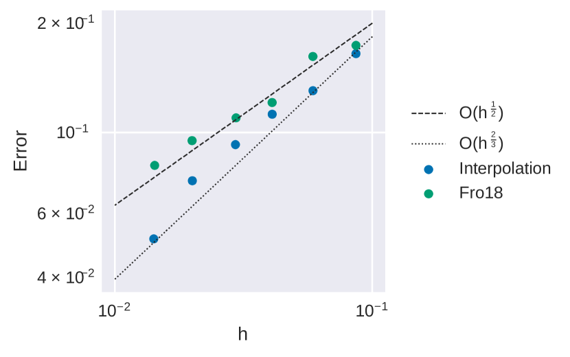
(a) Triangular mesh

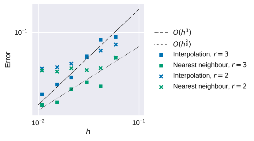
(b) Regular grid

Figure 4. Figure 4(a): Convergence plot for the convex envelope on the unit disc with triangular mesh. Figure 4(b): Convergence plot for the convex envelope on a regular grid over the square $[-1,1]^{2}$.

Triangular mesh, interpolation
$h$	$N$	Error	rate
$8.610-2$	427	0.16	–
$5.910-2$	785	0.13	0.61
$4.010-2$	1452	0.11	0.41
$2.910-2$	2713	0.09	0.58
$2.010-2$	5101	0.07	0.59
$1.410-2$	9674	0.05	1.07
Regular grid, interpolation, $r=2$
$h$	$N$	Error	rate
$5.910-2$	392	$7.510-2$	–
$4.110-2$	721	$6.510-2$	0.43
$3.010-2$	1288	$5.510-2$	0.51
$2.110-2$	2492	$4.710-2$	0.43
$1.510-2$	4616	$4.310-2$	0.26
$1.010-2$	9017	$4.210-2$	0.09
Regular grid, interpolation, $r=3$
$h$	$N$	Error	rate
$5.910-2$	528	$9.010-2$	–
$4.210-2$	913	$8.410-2$	0.20
$3.010-2$	1552	$5.610-2$	1.24
$2.110-2$	2868	$3.410-2$	1.45
$1.510-2$	5136	$2.910-2$	0.52
$1.010-2$	9757	$2.210-2$	0.68

Triangular mesh, Fro17
$h$	$N$	Error	rate
$8.610-2$	427	0.17	–
$5.010-2$	810	0.16	0.18
$4.110-2$	1533	0.12	0.80
$3.010-2$	2908	0.11	0.30
$2.010-2$	5526	0.09	0.37
$1.410-2$	10542	0.08	0.47
Regular grid, Nearest neighbour, $r=2$
$h$	$N$	Error	rate
$5.910-2$	392	$5.410-2$	–
$4.210-2$	721	$4.210-2$	0.73
$3.010-2$	1288	$4.010-2$	0.15
$2.110-2$	2492	$4.210-2$	-0.13
$1.510-2$	4616	$3.910-2$	0.24
$1.010-2$	9017	$4.010-2$	-0.07
Regular grid, Nearest neighbour, $r=3$
$h$	$N$	Error	rate
$5.910-2$	528	$5.410-2$	–
$4.210-2$	913	$2.710-2$	2.0
$3.010-2$	1552	$3.010-2$	-0.29
$2.110-2$	2868	$2.510-2$	0.47
$1.510-2$	5136	$1.910-2$	0.98
$1.010-2$	9757	$1.710-2$	0.18

Table 2. Errors and convergence order for the convex envelope.

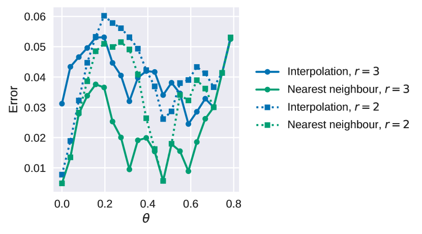
Figure 5. Error of the numerical solutions of the convex envelope PDE on a regular grid, as a function of rotation of the grid.

5.2. Pucci equation

Our next example is the Pucci equation,

(42) $$\begin{cases}\alpha\Lambda_{+}u(x)+\Lambda_{-}u(x)=0\qquad&x\in\Omega\\ u(x)=g(x)\qquad&x\in\partial\Omega\end{cases}$$

where $\alpha$ is a positive scalar, and $\Lambda_{-}u$ and $\Lambda_{+}u$ are respectively the minimal and maximal eigenvalues of the Hessian. A convergent, monotone and stable finite difference scheme for the Pucci equation was first developed in [Obe08b]. Following [DG05, Obe08b] we take

(43) $$u(x,y)=-\rho^{1-\alpha},\quad\rho(x,y)=\sqrt{(x+2)^{2}+(y+2)^{2}}.$$

We compute solutions on the unit disc and the square $[-1,1]^{2}$.

We discretized the square using a regular grid, and use either the nearest neighbour scheme, or the symmetric finite difference interpolation scheme presented in Section 3. We use stencils of radius two or three. Errors and rates of convergence on the grid are presented in Table 3 and in Figure 6(b). Both methods achieve roughly the same convergence rate before angular resolution error dominates. The nearest neighbour scheme achieves a slightly better error rate.

As in the convex envelope example, we used DistMesh to triangulate the unit disc. Error and convergence rates are shown Table 3 and Figure 6(a). Both methods achieve nearly $\mathcal{O}(1)$ convergence rate, which is better than predicted by our analysis. We hypothesize this is due to the fact that this example is smooth on the domain studied.

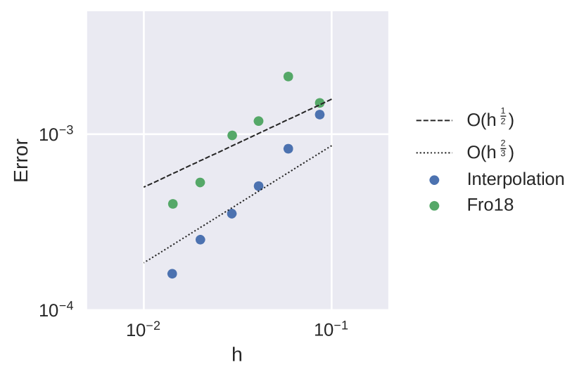
(a) Triangular mesh

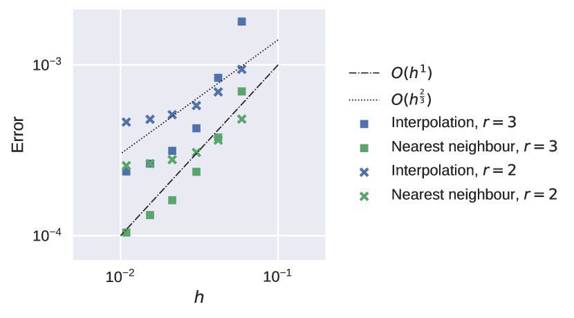
(b) Regular grid

Figure 6. Figure 6(a): Convergence plot for the Pucci equation on the unit disc with triangular mesh. Figure 6(b): Convergence plot for the Pucci equation on a regular grid over the square $[-1,1]^{2}$.

Triangular mesh, interpolation
$h$	$N$	Error	rate
$8.610-2$	427	$1.310-3$	–
$5.010-2$	785	$8.310-4$	1.16
$4.110-2$	1452	$5.010-4$	1.34
$3.010-2$	2713	$3.510-4$	1.09
$2.010-2$	5101	$2.510-4$	0.88
$1.410-2$	9674	$1.610-4$	1.29
Regular grid, interpolation, $r=2$
$h$	$N$	Error	rate
$5.910-2$	392	$9.410-4$	–
$4.110-2$	721	$7.010-4$	0.88
$3.010-2$	1288	$5.810-4$	0.58
$2.110-2$	2492	$5.110-4$	0.35
$1.510-2$	4616	$4.810-4$	0.19
$1.010-2$	9017	$4.610-4$	0.11
Regular grid, interpolation, $r=3$
$h$	$N$	Error	rate
$5.910-2$	528	$1.010-3$	–
$4.110-2$	913	$8.410-4$	2.20
$3.010-2$	1552	$4.210-4$	2.14
$2.110-2$	2868	$3.110-4$	0.86
$1.510-2$	5136	$2.610-4$	0.53
$1.010-2$	9757	$2.310-4$	0.30

Triangular mesh, Fro17
$h$	$N$	Error	rate
$8.610-2$	427	$1.510-3$	–
$5.010-2$	810	$2.110-3$	-0.90
$4.110-2$	1533	$1.210-3$	1.60
$3.010-2$	2908	$9.910-4$	0.58
$2.010-2$	5526	$5.310-4$	1.57
$1.410-2$	10542	$4.010-4$	0.841
Regular grid, Nearest neighbour, $r=2$
$h$	$N$	Error	rate
$5.910-2$	392	$4.810-4$	–
$4.110-2$	721	$3.610-4$	0.83
$3.010-2$	1288	$3.010-4$	0.52
$2.110-2$	2492	$2.810-4$	0.28
$1.510-2$	4616	$2.610-4$	0.16
$1.010-2$	9017	$2.610-4$	0.07
Regular grid, Nearest neighbour, $r=3$
$h$	$N$	Error	rate
$5.910-2$	528	$7.010-4$	–
$4.110-2$	913	$3.810-4$	1.80
$3.010-2$	1552	$2.410-4$	1.45
$2.110-2$	2868	$1.610-4$	1.08
$1.510-2$	5136	$1.310-4$	0.62
$1.010-2$	9757	$1.010-4$	0.68

Table 3. Errors and convergence order for the Pucci equation.

5.2.1. Solver comparison

Finally, we performed a comparison of the three solvers (semi-smooth Newton, Euler, and a combination of the two) in terms of CPU time, for the Pucci equation on a regular grid. Results are presented in Table 4.

As a function of number of grid points, the CPU time of Euler’s method is roughly $\mathcal{O}(N^{2})$ for both methods, interpolation and nearest neighbour. For the interpolation finite different schemes, both semi-smooth Newton and the combination solver is nearly $\mathcal{O}(N)$: we calculated a log-log line of best fit, and found semi-smooth Newton and the combination solver to be about $\mathcal{O}(N^{1.2})$.

Of all solvers and finite difference methods, the nearest neighbour finite difference scheme with the combination solver achieves the best CPU time, followed by the semi-smooth Newton. However, as a function of number of grid points, the CPU time is roughly $\mathcal{O}(N^{1.75})$. This rate is worse than the interpolation finite different scheme, and so we expect on even larger grids, eventually the interpolation finite difference method would be faster with either semi-smooth Newton or the combination solver.

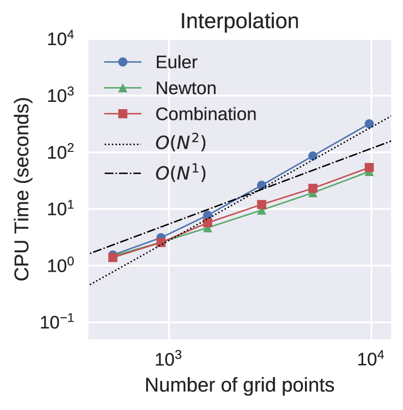
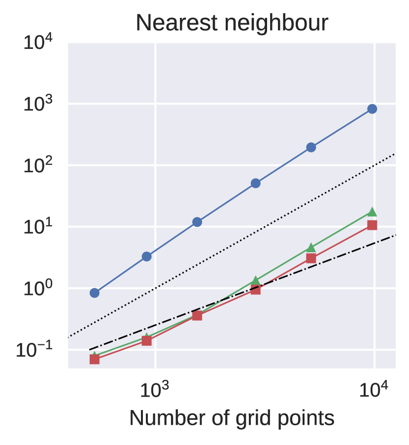
Figure 7. CPU time taken to compute solution of the Pucci equation on a regular grid, with stencil width $r=3$, for both methods.

Interpolation, $r=2$
$N$	392	721	1288	2492	4616	9017
Euler	1.16	3.22	9.43	34.39	125.49	500.98
Newton	0.74	1.29	2.70	5.86	12.32	28.86
Combination	0.75	1.36	2.50	6.07	12.39	28.35
Nearest neighbour, $r=2$
$N$	392	721	1288	2492	4616	9017
Euler	0.43	1.62	5.75	24.23	90.90	383.43
Newton	0.06	0.11	0.25	1.04	3.40	13.51
Combination	0.05	0.10	0.23	0.73	2.66	9.54
Interpolation, $r=3$
$N$	528	913	1552	2868	5136	9757
Euler	1.54	3.11	7.73	26.17	86.05	317.98
Newton	1.47	2.59	4.66	9.54	19.29	45.68
Combination	1.39	2.56	5.70	11.97	23.12	53.77
Nearest neighbour, $r=3$
$N$	528	913	1552	2868	5136	9757
Euler	0.84	3.28	11.93	50.90	195.14	823.99
Newton	0.08	0.16	0.37	1.35	4.63	17.66
Combination	0.07	0.14	0.36	0.95	3.07	10.61

Table 4. Comparison of wall clock time of solvers for the Pucci equation (42) in two dimensions on a regular grid. Time is reported in seconds. Results are for stencils of either radius $r=2$ or $r=3$.

References

- [BCM16] Jean-David Benamou, Francis Collino, and Jean-Marie Mirebeau. Monotone and consistent discretization of the monge-ampere operator. Mathematics of computation, 85(302):2743–2775, 2016.
- [BPR16] Olivier Bokanowski, Athena Picarelli, and Christoph Reisinger. High-order filtered schemes for time-dependent second order hjb equations. arXiv preprint arXiv:1611.04939, 2016.
- [BS91] Guy Barles and Panagiotis E. Souganidis. Convergence of approximation schemes for fully nonlinear second order equations. Asymptotic Anal., 4(3):271–283, 1991.
- [Car17] Rebecca M. Carrington. Speed Comparison of Solution Methods for the Obstacle Problem. Master’s thesis, McGill University, August 2017.
- [CIL92] Michael G. Crandall, Hitoshi Ishii, and Pierre-Louis Lions. User’s guide to viscosity solutions of second order partial differential equations. Bull. Amer. Math. Soc. (N.S.), 27(1):1–67, 1992.
- [CW17] Yangang Chen and Justin WL Wan. Multigrid methods for convergent mixed finite difference scheme for monge–ampère equation. Computing and Visualization in Science, pages 1–15, 2017.
- [CWL16] Yangang Chen, Justin WL Wan, and Jessey Lin. Monotone mixed finite difference scheme for monge–ampère equation. Journal of Scientific Computing, pages 1–29, 2016.
- [DB08] Germund Dahlquist and Åke Björck. Numerical methods in scientific computing, volume i. Society for Industrial and Applied Mathematics, 8, 2008.
- [DG05] Edward J Dean and Roland Glowinski. On the numerical solution of a two-dimensional pucci’s equation with dirichlet boundary conditions: a least-squares approach. Comptes Rendus Mathematique, 341(6):375–380, 2005.
- [FFL+17] Zexin Feng, Brittany D. Froese, Rongguang Liang, Dewen Cheng, and Yongtian Wang. Simplified freeform optics design for complicated laser beam shaping. Appl. Opt., 56(33):9308–9314, Nov 2017.
- [FM14] Jérôme Fehrenbach and Jean-Marie Mirebeau. Sparse Non-negative Stencils for Anisotropic Diffusion. Journal of Mathematical Imaging and Vision, 49(1):123–147, 2014.
- [FO13] Brittany D. Froese and Adam M. Oberman. Convergent filtered schemes for the Monge-Ampère partial differential equation. SIAM J. Numer. Anal., 51(1):423–444, 2013.
- [FP07] Francisco Facchinei and Jong-Shi Pang. Finite-dimensional variational inequalities and complementarity problems. Springer Science & Business Media, 2007.
- [Fro18] Brittany D. Froese. Meshfree finite difference approximations for functions of the eigenvalues of the hessian. Numerische Mathematik, 138(1):75–99, Jan 2018.
- [FS17] Brittany D Froese and Tiago Salvador. Higher-order Adaptive Finite Difference Methods for Fully Nonlinear Elliptic Equations. arXiv preprint arXiv:1706.07741, 2017.
- [Mir14a] J. Mirebeau. Anisotropic Fast-Marching on Cartesian Grids Using Lattice Basis Reduction. SIAM Journal on Numerical Analysis, 52(4):1573–1599, 2014.
- [Mir14b] Jean-Marie Mirebeau. Minimal Stencils for Monotony or Causality Preserving Discretizations of Anisotropic PDEs. 2014.
- [Mir16] Jean-Marie Mirebeau. Adaptive, anisotropic and hierarchical cones of discrete convex functions. Numerische Mathematik, 132(4):807–853, 2016.
- [NNZ17] Ricardo H Nochetto, Dimitrios Ntogkas, and Wujun Zhang. Two-scale method for the monge-ampere equation: Pointwise error estimates. arXiv preprint arXiv:1706.09113, 2017.
- [NSZ17] Michael Neilan, Abner J. Salgado, and Wujun Zhang. Numerical analysis of strongly nonlinear pdes. Acta Numerica, 26:137–303, 2017.
- [Obe06] Adam M. Oberman. Convergent difference schemes for degenerate elliptic and parabolic equations: Hamilton-Jacobi equations and free boundary problems. SIAM J. Numer. Anal., 44(2):879–895 (electronic), 2006.
- [Obe07] Adam Oberman. The convex envelope is the solution of a nonlinear obstacle problem. Proceedings of the American Mathematical Society, 135(6):1689–1694, 2007.
- [Obe08a] Adam M Oberman. Computing the convex envelope using a nonlinear partial differential equation. Mathematical Models and Methods in Applied Sciences, 18(05):759–780, 2008.
- [Obe08b] Adam M Oberman. Wide stencil finite difference schemes for the elliptic Monge-Ampere equation and functions of the eigenvalues of the Hessian. Discrete Contin. Dyn. Syst. Ser. B, 10(1):221–238, 2008.
- [OS15] Adam M Oberman and Tiago Salvador. Filtered schemes for Hamilton–Jacobi equations: A simple construction of convergent accurate difference schemes. J. Comput. Phys., 284:367–388, 2015.
- [OZ16] Adam M Oberman and Ian Zwiers. Adaptive finite difference methods for nonlinear elliptic and parabolic partial differential equations with free boundaries. Journal of Scientific Computing, 68(1):231–251, 2016.
- [PS04] Per-Olof Persson and Gilbert Strang. A simple mesh generator in matlab. SIAM review, 46(2):329–345, 2004.