Heterogeneous inputs to central pattern generators
can shape insect gaits.

Abstract

In our previous work [1], we studied an interconnected bursting neuron model for insect locomotion, and its corresponding phase oscillator model, which at high speed can generate stable tripod gaits with three legs off the ground simultaneously in swing, and at low speed can generate stable tetrapod gaits with two legs off the ground simultaneously in swing. However, at low speed several other stable locomotion patterns, that are not typically observed as insect gaits, may coexist. In the present paper, by adding heterogeneous external input to each oscillator, we modify the bursting neuron model so that its corresponding phase oscillator model produces only one stable gait at each speed, specifically: a unique stable tetrapod gait at low speed, a unique stable tripod gait at high speed, and a unique branch of stable transition gaits connecting them. This suggests that control signals originating in the brain and central nervous system can modify gait patterns.

Key words. insect gaits, bursting neurons, phase reduction, coupling functions, phase response curves, bifurcation, unfolding, stability

AMS subject classifications. 34C15, 34C60, 37G10, 92B20, 92C20

1 Introduction

This paper is based on our previous work [1], in which we studied the effect of stepping frequency on transitions from multiple tetrapod insect gaits with two legs off the ground simultaneously in swing, to tripod gaits with three legs off the ground simultaneously in swing. In that paper, we used an ion-channel bursting neuron model to describe each of six mutually inhibitory units that form the central pattern generator (CPG) located in the insect’s thorax. We assumed that each unit drives one leg of the insect and that the units are connected to their nearest neighbors in a homogeneous network as shown in Figure 2 below, but where input currents are identical, $I_{i}=I_{ext}$.

Employing phase reduction, we collapsed the network of bursting neurons represented by 24 ordinary differential equations to 6 coupled nonlinear phase oscillators, each corresponding to a sub-network of neurons controlling one leg. Assuming that the left and right legs maintain constant phase differences (contralateral symmetry), we reduced from 6 equations to 3, allowing analysis of a dynamical system with 2 phase differences defined on a 2-dimensional torus.

With certain balance conditions on the coupling strengths among the homogeneous oscillators, described in Section 4 below, we showed that at low speeds, the phase differences model on the torus can generate multiple fixed points, including stable tetrapod and unstable tripod gaits. In contrast, at high speeds, it generates a unique stable tripod gait. Moreover, as speed increases, the gait transition occurs through degenerate bifurcations, at which a subset of the multiple fixed points merge to produce a unique stable fixed point [1, Figure 23].

In the current paper, we study this degenerate bifurcation in the phase difference model, by unfolding the original system. To this end we relax the condition of homogeneous (identical) ion-channel bursting neuron models in the network of CPGs and allow heterogeneous (nonidentical) models by adding different external inputs to each oscillator. We subsequently show that this heterogeneity is equivalent to perturbing the coupling functions or the contralateral coupling strengths in a phase reduced oscillator model; i.e. different heterogeneities can have the same effects on dynamics. (see Section 6 below).

The paper is organized as follows. In Section 2, we review the ion-channel model for bursting neurons which was developed in [2, 3], and the influence of its parameters on speed, which was studied in [1]. In Section 3, we review the derivation of phase equations for heterogeneous networks and apply these techniques to the interconnected bursting neuron model. In Section 4, we define approximate tetrapod, tripod and transition gaits for heterogeneous networks and then, by assuming constant phase differences between left- and right-hand oscillators, as in the homogeneous case, we reduce the 6 phase equations to 2 phase difference equations. In Section 5, we describe the main results of this paper. By choosing appropriate heterogeneous external inputs, we show that the phase differences model generates only one stable fixed point, which at low speed, corresponds to a tetrapod gait and at high speed, corresponds to a tripod gait. Interpreting the heterogeneities as small bifurcation parameters, we find cases in which two or three saddle-node bifurcations occur as heterogeneity increases and a unique tetrapod gait emerges from multiple tetrapod gaits and other, ill-defined gaits. This shows that specific fixed points (gaits) can be preserved, or removed, by small external input currents. In Section 6, we show that our heterogeneities are equivalent to perturbing the coupling functions or the contralateral coupling strengths in a phase reduced oscillator model. In Section 7, we conclude.

2 A network of weakly interconnected bursting neurons

In [1, Section 2.1], we employed an ion-channel bursting neuron model for an insect central pattern generator which was developed in [2, 3]. The bursting neuron model of each unit of the CPG contains a system of 4 ODEs describing trans-membrane cell voltages, slow and fast ionic gates, and the dynamics of neurotransmitter release at synapses, as follows:

$$C\dot{v} =-\left\{I_{Ca}(v)+I_{K}(v,m)+I_{KS}(v,{w})+I_{L}(v)\right\}+I_{ext},$$ (1a)

$$\dot{m} =\displaystyle\frac{\gamma}{\tau_{m}(v)}[m_{\infty}(v)-m],$$ (1b)

$$\dot{{w}} =\displaystyle\frac{\delta}{\tau_{{w}}(v)}[{w}_{\infty}(v)-{w}],$$ (1c)

$$\dot{s} =\displaystyle\frac{1}{\tau_{s}}[s_{\infty}(v)(1-s)-s],$$ (1d)

where the ionic currents are of the following forms

$$I_{Ca}(v)\;=\;\bar{g}_{Ca}n_{\infty}(v)(v-E_{Ca}),\qquad I_{K}(v,m)\;=\;\bar{g}_{K}\;m\;(v-E_{K}),$$ (2)

$$I_{KS}(v,{w})\;=\;\bar{g}_{KS}{w}\;(v-E_{KS}),\qquad I_{L}(v)\;\;=\;\;\bar{g}_{L}(v-E_{L}).$$

The steady state gating variables associated with ion channels and their time scales take the forms

$$m_{\infty}(v)\;=\;\frac{1}{1+e^{-2k_{K}(v-v_{K})}}\;,\qquad\qquad{w}_{\infty}(v)\;=\;\frac{1}{1+e^{-2k_{KS}(v-v_{KS})}}\;,$$ (3)

$$n_{\infty}(v)\;=\;\frac{1}{1+e^{-2k_{Ca}(v-v_{Ca})}}\;,\qquad\qquad s_{\infty}(v)\;=\;\frac{a}{1+e^{-2k_{s}(v-E^{pre}_{s})}}\;,$$

and

$$\tau_{m}(v)=\mbox{sech}\,(k_{K}(v-v_{K})),\quad\tau_{{w}}(v)=\mbox{sech}\,(k_{KS}(v-v_{KS})).$$ (4)

The external current $I_{ext}$, which represents input from the central nervous system and brain, varies between $35.65$ and $37.7$ as speed increases. Other parameters are generally fixed as specified in Table 1 and are chosen such that the model (1) possesses an attracting hyperbolic limit cycle $\Gamma$. Most of the parameter values are taken from [3], but some of our notations are different. See [1, Section 2.1] for further details of the model and its parameters.

$I_{ext}$	$\bar{g}_{Ca}$	$\bar{g}_{K}$	$\bar{g}_{KS}$	$\bar{g}_{L}$	$\bar{g}_{syn}$	$E_{Ca}$	$E_{K}$	$E_{KS}$	$E_{L}$	$E^{post}_{s}$	$E^{pre}_{s}$
varies	4.4	9.0	0.5	2.0	0.01	120	-80	-80	-60	-70	2

$k_{Ca}$	$k_{K}$	$k_{KS}$	$k_{s}$	$v_{Ca}$	$v_{K}$	$v_{KS}$	a	$C$	$\gamma$	$\tau_{s}$	$\delta$
0.056	0.1	0.8	0.11	-1.2	2	-26	444.48	1.2	5.0	5.56	0.027

Table 1: The constant parameters in the bursting neuron model.

As shown in Figure 1(left), the periodic orbit in $(v,m,{w})$ space contains a sequence of spikes (a burst) followed by a quiescent phase, which correspond respectively to the swing and stance durations of one leg. The burst from the CPG inhibits depressor motoneurons and excites levator motoneurons, allowing the swing leg to lift from the ground [2, Figure 2] and [4, Figure 11] (see also [5, 6]). We denote the period of the periodic orbit by $T$, i.e., it takes $T$ time units (ms here) to complete the stance and swing cycle of each leg. The number of steps completed by one leg per unit of time is the stepping frequency and is equal to $\omega=2\pi/T$. In [1, Figure 2], we observed that as one of the two parameters in the bursting neuron model, either the slow time scale $\delta$ or the external current $I_{ext}$, increases, the period of the periodic orbit decreases, primarily by decreasing stance duration, and so the insect’s speed increases. There, we used these parameters as speed parameters, denoted by ${\xi}$, and studied transitions from tetrapod to tripod gaits as ${\xi}$ increases. Gait transition is not the main focus of the present paper, although here we will show gait transitions using only $I_{ext}$ as a speed parameter. To see how $I_{ext}$ affects the frequency of the periodic orbit, see Figure 1(right).

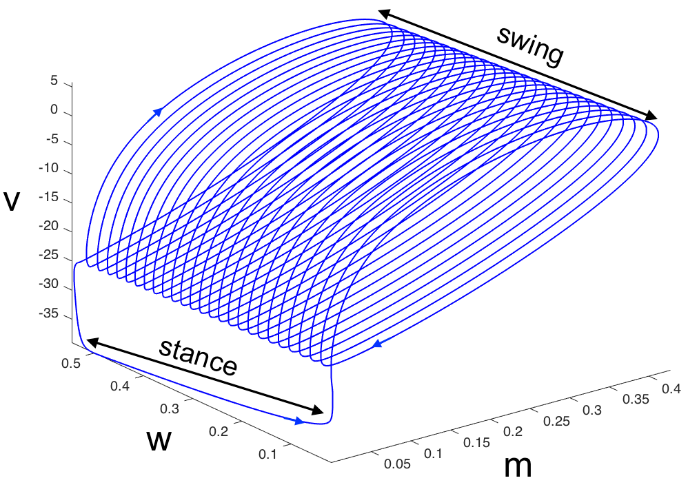
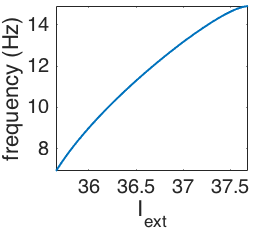
Figure 1: Left: A periodic orbit of the bursting neuron model, Equation (1), in $(v,m,{w})$ space. Right: The effect of $I_{ext}$ on the stepping frequency of the periodic orbit.

In [1], we assumed that inhibitory coupling is achieved via synapses that produce negative postsynaptic currents. The synapse variable $s$ enters the postsynaptic cell in Equation (1a) as an additional term, $I_{syn}$,

$$C\dot{v}_{i} =-\left\{I_{Ca}+I_{K}+I_{KS}+I_{L}\right\}+I_{ext}+I_{syn}\;,$$ (5)

where

$$I_{syn}=\sum_{j\in\mathcal{N}_{i}}I_{syn}(v_{i},s_{j})=\sum_{j\in\mathcal{N}_{i}}-\bar{c}_{ji}\bar{g}_{syn}s_{j}\left(v_{i}-E_{s}^{post}\right),$$ (6)

$\bar{g}_{syn}$ denotes the synaptic strength, and $\mathcal{N}_{i}$ denotes the set of the nodes adjacent to node $i$. The multiplicative factor $\bar{c}_{ji}$ accounts for the fact that multiple bursting neurons are interconnected in the insects, and $-\bar{c}_{ji}\bar{g}_{syn}$ represents an overall coupling strength between hemi-segments. Following [7] we assumed contralateral symmetry and included only nearest neighbor coupling, so that there are three contralateral coupling strengths ${c}_{1},{c}_{2},{c}_{3}$ and four ipsilateral coupling strengths ${c}_{4},{c}_{5},{c}_{6},$ and ${c}_{7}$; see Figure 2. For example, $\bar{c}_{21}={c}_{5}$, $\bar{c}_{41}={c}_{1},$ etc. We chose reversal potentials $E^{post}_{s}$ that make all synaptic connections inhibitory; this implies that the $c_{i}$’s are positive.

The following system of $24$ ordinary differential equations (ODEs) describes the dynamics of the $6$ coupled cells in the network as shown in Figure 2. We assume that each cell, which is governed by Equation (1), represents one leg of the insect. Cells $1,2$, and $3$ represent right front, middle, and hind legs, and cells $4,5$, and $6$ represent left front, middle, and hind legs, respectively:

$$\begin{array}[]{ll}&\dot{x}_{1}\;=\;f(x_{1})+{c}_{1}g(x_{1},x_{4})+{c}_{5}g(x_{1},x_{2}),\\ &\dot{x}_{2}\;=\;f(x_{2})+{c}_{2}g(x_{2},x_{5})+{c}_{4}g(x_{2},x_{1})+{c}_{7}g(x_{2},x_{3}),\\ &\dot{x}_{3}\;=\;f(x_{3})+{c}_{3}g(x_{3},x_{6})+{c}_{6}g(x_{3},x_{2}),\\ &\dot{x}_{4}\;=\;f(x_{4})+{c}_{1}g(x_{4},x_{1})+{c}_{5}g(x_{4},x_{5}),\\ &\dot{x}_{5}\;=\;f(x_{5})+{c}_{2}g(x_{5},x_{2})+{c}_{4}g(x_{5},x_{4})+{c}_{7}g(x_{5},x_{6}),\\ &\dot{x}_{6}\;=\;f(x_{6})+{c}_{3}g(x_{6},x_{3})+{c}_{6}g(x_{6},x_{5}),\end{array}$$ (7)

where $x_{i}=(v_{i},m_{i},{w}_{i},s_{i})^{\top}$, $f(x_{i})$ is as the right hand side of Equations (1) and

$$g(x_{i},x_{j})=\left(-\bar{g}_{syn}s_{j}\left(v_{i}-E_{s}^{post}\right),0,0,0\right)^{\top},$$ (8)

is the coupling function with a small synaptic coupling strength $\bar{g}_{syn}$. This assumption of weak coupling is necessary for the use of phase reduction in Section 3.

This 6-bursting neuron model was used to drive agonist-antagonist muscle pairs in a neuro-mechanical model with jointed legs that reproduced the dynamics of freely-running cockroaches [8], also see [14]. These papers and subsequent phase-reduced models [15, 7] support our belief that the bursting neuron model is capable of producing realistic inputs to muscles in insects. In [1, Figures 5 and 6], we showed that the 24 ODEs coupled bursting neuron model with small $I_{ext}$ (or $\delta$) can produce a tetrapod gait with two legs lifted off the ground simultaneously in swing; and as $I_{ext}$ (or $\delta$) increases, it can produce a tripod gait with three legs lifted off the ground simultaneously in swing.

In [1, Section 2.2] we considered a network of six identical mutually inhibiting homogeneous units, representing the hemi-segmental CPG networks contained in the insect’s thorax. In the present paper, we assume that in addition to $I_{ext}$, each unit receives a different external input denoted by ${I_{ext}^{i}(t)}$, as shown in Figure 2, where ${I_{ext}^{i}(t)}$ is a periodic function with frequency $\omega_{i}$ close to $\omega$ and a magnitude of order $\mathcal{O}(\bar{g}_{syn})$, and $\bar{g}_{syn}$ is the synaptic strength. Therefore, in all the previous equations, $I_{ext}$ will be replaced by $I_{ext}+{I_{ext}^{i}(t)}$, where $i$ denotes the leg number. Later we also assume that for $i=1,2,3$, ${I_{ext}^{i}(t)}=I_{ext}^{i+3}$, to preserve the contralateral symmetry condition; see Assumption 2 in Section 4.

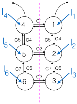
Figure 2: The network of heterogeneous CPGs with different external inputs, $I_{i}=I_{ext}+I^{i}_{ext}(t)$.

To analyze the gait transition mathematically, in [1, Section 3], we applied the theory of weakly coupled oscillators to the coupled bursting neuron models to reduce the 24 ODEs to 6 phase oscillator equations. In the following section we apply the phase reduction technique again and derive 6 phase oscillator equations in the presence of heterogeneous external inputs.

3 A phase oscillator model

Let the ODE

$$\dot{x}=f(x),\qquad x\in{\mathbb{R}}^{n},$$ (9)

describe the dynamics of a single oscillator. Assume that Equation (9) has an attracting hyperbolic limit cycle $\Gamma=\Gamma(t)$, with period $T$ and frequency ${\omega}=2\pi/T$. The phase of an oscillator, denoted by $\phi$, is the time that has elapsed as its state moves around $\Gamma$, starting from an arbitrary reference point in the cycle, called relative phase. In this section, we derive the phase equations of weakly coupled oscillators with heterogeneous dynamics, i.e., coupled oscillators with different frequencies. We develop the theory in greater generality than our specific applications will demand, allowing periodic input currents $I^{i}_{ext}(t)$.

3.1 A pair of weakly coupled heterogeneous oscillators

Consider a pair of weakly coupled heterogeneous oscillators

$$\dot{x}_{1}=f_{1}(x_{1})+\epsilon g(x_{1},x_{2}),$$ (10)

$$\dot{x}_{2}=f_{2}(x_{2})+\epsilon g(x_{2},x_{1}),$$

where $f_{i}$ describes the intrinsic dynamics of each oscillator, $0<\epsilon\ll 1$ is the coupling strength, and $g$ is the coupling function. For each oscillator, the phase equation can be written as follows. For more details see [1, Section 3].

$$\frac{d\phi_{i}}{dt}(t)=\omega_{i}+\epsilon H_{i}(\phi_{j}(t)-\phi_{i}(t))+\mathcal{O}(\epsilon^{2}),$$ (11)

where

$$H_{i}=H_{i}(\theta)=\frac{1}{T}\int_{0}^{T}Z_{i}(\Gamma_{i}(\tilde{t}))\cdot g(\Gamma_{i}(\tilde{t}),\Gamma_{i}(\tilde{t}+\theta))\;d\tilde{t},$$

is the coupling function: the convolution of the coupling $g$ and the oscillator’s infinitesimal phase response curve (iPRC), $Z_{i}$, and $\omega_{i}$ is the frequency of each oscillator described by $\dot{x}_{i}=f_{i}(x_{i})$. Under the weak coupling assumption, the iPRC captures the local dynamics of each oscillator in a neighborhood of its limit cycle $\Gamma_{i}$, [9].

Equation (11) is a general phase equation for a pair of weakly coupled heterogeneous oscillators where the heterogeneity is of any arbitrary size. This means that the oscillators’ frequencies can be very different from each other. But if the frequencies are close to each other, i.e, the heterogeneities are small and in particular are of order of the coupling strength $\epsilon$, then one can approximate Equation (11) as follows [10, Chapter 5].

Assume that $f_{i}=f+\tilde{f}_{i}$, where the heterogeneity $\tilde{f}_{i}$ is periodic with period close to the period of $f$ and $\tilde{f}_{i}$ is of order $\epsilon,\mathcal{O}(\epsilon)$. This is equivalent to having identical oscillators with dynamics $f$ and non-identical coupling functions $g_{i}=g+\tilde{f}_{i}/\epsilon$. Then Equation (11) can be approximated by the following phase equations:

$$\frac{d\phi_{i}}{dt}(t)=\omega+\tilde{\omega}_{i}+\epsilon H(\phi_{j}(t)-\phi_{i}(t))+\mathcal{O}(\epsilon^{2}),$$ (12)

where

$$H=H(\theta)=\frac{1}{T}\int_{0}^{T}Z(\Gamma(\tilde{t}))\cdot g(\Gamma(\tilde{t}),\Gamma(\tilde{t}+\theta))\;d\tilde{t},$$

is a coupling function: specifically, the convolution of the synaptic coupling $g$ and the oscillator’s infinitesimal phase response curve (iPRC), $Z$. Here $Z$ is computed for the limit cycle of $\dot{x}=f(x)$, and the frequency differences are constant shifts of $\mathcal{O}(\epsilon)$:

$$\tilde{\omega}_{i}=\frac{1}{T}\int_{0}^{T}Z(\Gamma(\tilde{t}))\cdot\tilde{f}_{i}(\Gamma(\tilde{t}))\;d\tilde{t}.$$ (13)

The advantage of this decomposition is that only one iPRC and so only one coupling function need to be computed.

In what follows we generalize the approximation of Equation (12) to a network of weakly coupled heterogeneous neurons with multiple connections [10, Chapter 5].

3.2 A network of weakly coupled heterogeneous oscillators

Now consider a network of $N$ heterogeneous oscillators with intrinsic dynamics $\dot{x}_{i}=f_{i}(x_{i})$ and corresponding frequencies $\omega_{i}$. For $i=1,\ldots,N$, let

$$\dot{x}_{i}=f_{i}(x_{i})+\sum_{j\in\mathcal{N}_{i}}\epsilon_{j}g(x_{i},x_{j}),$$ (14)

describe the dynamics of each $x_{i}$ in the weakly coupled network. Here $\mathcal{N}_{i}$ denotes the neighbors of oscillator $i$, and $\epsilon_{j}$ denotes the coupling strengths, which are all of $\mathcal{O}(\epsilon)$ for some $0<\epsilon\ll 1$. As in the case of a pair of coupled oscillators, one can derive phase equations from Equation (14) as follows

$$\dot{\phi}_{i}=\omega_{i}+\sum_{j\in\mathcal{N}_{i}}\epsilon_{j}H_{j}(\phi_{j}-\phi_{i})+\mathcal{O}(\epsilon^{2}),$$ (15)

where the coupling function $H_{j}$ is the convolution of the coupling function $g$ and each oscillator’s iPRC, $Z_{i}$.

Now, similar to Equation (12), we approximate Equation (15) such that all the coupling functions can be computed from a single iPRC which corresponds to the limit cycle of $\dot{x}=f(x)$. Assume that $f_{i}=f+\tilde{f}_{i}$, where $\tilde{f}_{i}$ is periodic with period close to the period of $f$, and $\tilde{f}_{i}$ is of $\mathcal{O}(\epsilon)$. As in the case of a pair of coupled neurons, since the perturbation $\tilde{f}_{i}=\mathcal{O}(\epsilon)$, we can approximate each limit cycle by the limit cycle of $\dot{x}=f(x)$ and consider $\tilde{f}_{i}$ as a perturbation to the coupling function $g$. Therefore, Equation (15) can be written as

$$\dot{\phi}_{i}=\omega+\tilde{\omega}_{i}+\sum_{j\in\mathcal{N}_{i}}\epsilon_{j}H(\phi_{j}-\phi_{i})+\mathcal{O}(\epsilon^{2}),$$ (16)

where $\omega$ is the frequency of the limit cycle of $\dot{x}=f(x)$, $H$ is the convolution of the coupling function $g$ and $Z$, the iPRC of the limit cycle of $\dot{x}=f(x)$, and the frequency differences are

$$\tilde{\omega}_{i}\;=\;\frac{1}{T}\int_{0}^{T}Z(\Gamma(\tilde{t}))\cdot\tilde{f}_{i}(\Gamma(\tilde{t}))\;d\tilde{t}.$$ (17)

3.3 Phase equations for six weakly coupled heterogeneous bursting neuron model

We now apply the techniques from Section 3.2 to six heterogeneous units in the coupled bursting neuron model and derive the 6-coupled phase oscillator model via phase reduction.

In the interconnected bursting neuron model, Equation (7), the intrinsic dynamics of each hemi-segmental unit, described by $\dot{x}=f(x)$, is homogeneous. We now assume that each hemi-segmental unit receives a small heterogeneous external input, i.e., each unit can be described by

$$\dot{x}_{i}=f_{i}(x_{i})=f(x_{i})+{I_{ext}^{i}(t)}\cdot\mathbf{e}_{1},$$

where $\dot{x}_{i}=f_{i}(x_{i})$ has an attracting hyperbolic limit cycle with frequency close to the attracting hyperbolic limit cycle of $\dot{x}=f(x)$. For $i=1,\ldots,6$, ${I_{ext}^{i}(t)}$ is the additional small external input to each unit and represents the weak heterogeneity of the corresponding unit such that ${I_{ext}^{i}(t)}=\mathcal{O}(\bar{g}_{syn})$ and $\mathbf{e}_{1}=(1,0,0,0)^{\top}$, i.e., only the voltage equations are heterogeneous.

Recalling Equation (16), we can derive approximate phase equations for the coupled bursting neuron model of Figure 2 as follows.

$$\begin{array}[]{ll}&\dot{\phi}_{1}\;=\;\omega+\tilde{\omega}_{1}+{c}_{1}H(\phi_{4}-\phi_{1})+{c}_{5}H(\phi_{2}-\phi_{1}),\\ &\dot{\phi}_{2}\;=\;\omega+\tilde{\omega}_{2}+{c}_{2}H(\phi_{5}-\phi_{2})+{c}_{4}H(\phi_{1}-\phi_{2})+{c}_{7}H(\phi_{3}-\phi_{2}),\\ &\dot{\phi}_{3}\;=\;\omega+\tilde{\omega}_{3}+{c}_{3}H(\phi_{6}-\phi_{3})+{c}_{6}H(\phi_{2}-\phi_{3}),\\ &\dot{\phi}_{4}\;=\;\omega+\tilde{\omega}_{4}+{c}_{1}H(\phi_{1}-\phi_{4})+{c}_{5}H(\phi_{5}-\phi_{4}),\\ &\dot{\phi}_{5}\;=\;\omega+\tilde{\omega}_{5}+{c}_{2}H(\phi_{2}-\phi_{5})+{c}_{4}H(\phi_{4}-\phi_{5})+{c}_{7}H(\phi_{6}-\phi_{5}),\\ &\dot{\phi}_{6}\;=\;\omega+\tilde{\omega}_{6}+{c}_{3}H(\phi_{3}-\phi_{6})+{c}_{6}H(\phi_{5}-\phi_{6}),\end{array}$$ (18)

where

$$\tilde{\omega}_{i}=\frac{1}{T}\int_{0}^{T}Z_{v}(\Gamma(t))I_{ext}^{i}(t)dt,$$ (19)

and $Z_{v}$ is the iPRC of the limit cycle of $\dot{x}=f(x)$ in the direction of voltage. In Figure 3 (left), we show $Z_{v}$ for $I_{ext}=35.9$. Note that the averaging theorem and convolution integral in phase reduction eliminates time dependence in $I^{i}_{ext}$. Also, the coupling function $H$ takes the following form:

$$H(\theta)=-\frac{\bar{g}_{syn}}{T}\int_{0}^{T}Z_{v}(\Gamma(t))\left(v_{i}(\Gamma(t))-E_{s}^{post}\right)s_{j}\left(\Gamma(t+\theta)\right)\;dt.$$ (20)

In Figure 3 (right), we show the coupling function $H$ derived in Equation (20) for $I_{ext}=35.9$. Note that $H(\theta)<0$ over most of its range, and in particular over the interval $[1/3,2/3]$, which we will show contains the tetrapod, tripod and transition gaits.

To simplify the notations, for the remainder of the paper, $T=1$ and all the phases and the coupling functions are considered in the domain of $[0,1]$ instead of $[0,2\pi]$.

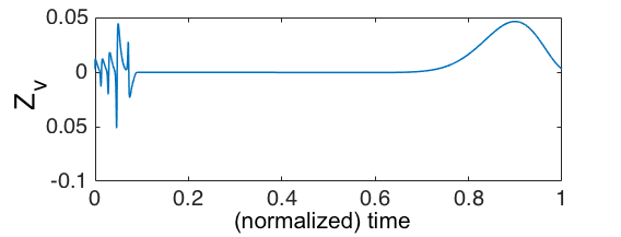
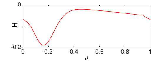
Figure 3: [1, Figure 8] iPRC (in the direction of $v$) (left) and the coupling function $H(\theta)$ (right) for $I_{ext}=35.9$. Phase $\theta=0$ is defined to be the onset of the burst.

4 Reduced phase equations

In this section, the goal is to reduce the 6 equations (18) to 2 equations on a 2-torus. Although we are interested in gaits generated by the bursting neuron model and its phase reduction equations (18), we prove our results for a more general case. To this end, we assume the following conditions for the coupling function $H$ and the external inputs ${I_{ext}^{i}(t)}$. We let the coupling function $H$ and the frequency $\omega$ depend on the speed parameter ${\xi}$ and write $H=H(\phi;{\xi})$ and $\omega=\omega({\xi})$.

Assumption 1.

Let $H=H(\theta;{\xi})$ be a differentiable function, defined on ${\mathbb{R}}\times[{\xi}_{1},{\xi}_{2}]$ which is $1$-periodic on its first argument and has the following property. For any fixed ${\xi}\in[{\xi}_{1},{\xi}_{2}]$,

$$H\left(\frac{2}{3}-{\eta};{\xi}\right)=H\left(\frac{1}{3}+{\eta};{\xi}\right),$$ (21)

has a unique solution $\eta({\xi})$ such that $\eta=\eta({\xi}):[{\xi}_{1},{\xi}_{2}]\to[0,1/6]$ is an onto and non-decreasing function. Note that Equation (21) is also trivially satisfied by the constant solution ${\eta}=1/6$.

Assumption 1 defines a class of coupling functions that exhibit the gait transitions studied here and in [1]. The coupling functions derived from the bursting neuron model satisfy and motivate this assumption, see [1, Figure 9]. For the rest of the paper, we assume that the coupling function $H$ satisfies Assumption 1. In [1, Proposition 11], we provided sufficient conditions for Assumption 1 to hold for more general classes of functions.

Assumption 2.

For $i=1,2,3$, let $I_{ext}^{i+3}(t)={I_{ext}^{i}(t)}$. This assumption maintains contralateral symmetry. In addition, we assume that for $i=1,2,3$, ${I_{ext}^{i}(t)}$ are not equal, otherwise the system becomes homogeneous.

Assumption 3.

Let the coupling strengths satisfy the following balance condition

$${c}_{1}+{c}_{5}={c}_{2}+{c}_{4}+{c}_{7}={c}_{3}+{c}_{6}.$$ (22)

In [1, Proposition 3 and Corollary 4] we proved that when the coupling strengths satisfy the balance condition, in the homogeneous case $\tilde{\omega}_{i}=0$, Equation (18) admits tetrapod gaits at low speeds and tripod gaits at high speeds.

4.1 Gait definitions: Generalization to heterogeneous systems

In [1, Definition 1] we defined four versions of tetrapod gaits and a tripod gait. Each gait corresponded to a $1$-periodic solution of Equation (18) with $\tilde{\omega}_{i}=0$. In what follows, we generalize those definitions to heterogeneous models, i.e., Equation (18) with at least one $\tilde{\omega}_{i}\neq 0$.

Definition 1 (Approximate tetrapod and tripod gaits).

The approximate gaits, denoted by $A_{T}^{p}$, are $1$-periodic solutions of Equation (18) with at least one $\tilde{\omega}_{i}\neq 0$:

$$A_{T}^{p}:=\left(\hat{\omega}t+\psi_{1}+{\delta}_{1},\;\hat{\omega}t+\psi_{2}+{\delta}_{2},\;\hat{\omega}t+\psi_{3}+{\delta}_{3};\;\;\hat{\omega}t+\psi_{1}+{\delta}_{1}+\psi,\;\hat{\omega}t+\psi_{2}+{\delta}_{2}+\psi,\;\hat{\omega}t+\psi_{3}+{\delta}_{3}+\psi\right)^{\top},$$

where $\hat{\omega}$ is a coupled stepping frequency that all six oscillators share

$$\hat{\omega} =\omega({\xi})+{c}_{1}H\left(\psi;{\xi}\right)+{c}_{5}H(\psi_{2}-\psi_{1};{\xi})$$ (23)

$$=\omega({\xi})+{c}_{2}H\left(\psi;{\xi}\right)+{c}_{4}H(\psi_{1}-\psi_{2};{\xi})+{c}_{7}H\left(\psi_{3}-\psi_{2};{\xi}\right)$$

$$=\omega({\xi})+{c}_{3}H\left(\psi;{\xi}\right)+{c}_{6}H\left(\psi_{2}-\psi_{3};{\xi}\right),$$

$\psi_{1},\psi_{2},\psi_{3}$ are corresponding relative phases, and $\psi$ is the corresponding constant contralateral phase difference in approximate gaits. Note that the equalities in $\hat{\omega}$ hold by Assumptions 1 and 3.

The ${\delta}_{i}$’s are perturbations to the legs’ phases due to the heterogeneity and are the solutions of

$$\left(\begin{array}[]{c}\tilde{\omega}_{1}\\ \tilde{\omega}_{2}\\ \tilde{\omega}_{3}\end{array}\right)=\mathcal{L}(\psi_{1},\psi_{2},\psi_{3})\left(\begin{array}[]{c}{\delta}_{1}\\ {\delta}_{2}\\ {\delta}_{3}\end{array}\right),$$

where

$$\mathcal{L}(\psi_{1},\psi_{2},\psi_{3})=\left(\begin{array}[]{ccc}{c}_{5}H^{\prime}(\psi_{2}-\psi_{1};{\xi})&-{c}_{5}H^{\prime}(\psi_{2}-\psi_{1};{\xi})&0\\ -{c}_{4}H^{\prime}(\psi_{1}-\psi_{2};{\xi})&{c}_{4}H^{\prime}(\psi_{1}-\psi_{2};{\xi})+{c}_{7}H^{\prime}(\psi_{3}-\psi_{2};{\xi})&-{c}_{7}H^{\prime}(\psi_{3}-\psi_{2};{\xi})\\ 0&-{c}_{6}H^{\prime}(\psi_{2}-\psi_{3};{\xi})&{c}_{6}H^{\prime}(\psi_{2}-\psi_{3};{\xi})\end{array}\right),$$

and $H^{\prime}$ denotes the derivative of $H$ w.r.t. its first argument. The matrix $\mathcal{L}$ is singular, so we let $(\delta_{1},\delta_{2},\delta_{3})^{\top}=\mathcal{L}^{+}(\tilde{\omega}_{1},\tilde{\omega}_{2},\tilde{\omega}_{3})^{\top}$, where $\mathcal{L}^{+}$ is the generalized inverse (pseudoinverse) of $\mathcal{L}$, see [11].

The following choices of the relative phases $\psi_{1},\psi_{2},\psi_{3}$, and the contralateral phase difference $\psi$ give four different versions of approximate tetrapod gaits and an approximate tripod gait.

1. The approximate forward right tetrapod gait, denoted by $A_{FR}^{p}$, corresponds to $A_{T}^{p}$ with $\psi_{1}=2/3,\psi_{2}=0,\psi_{3}=1/3$, and $\psi=2/3$.

2. The approximate forward left tetrapod gait, denoted by $A_{FL}^{p}$, corresponds to $A_{T}^{p}$ with $\psi_{1}=2/3,\psi_{2}=0,\psi_{3}=1/3$, and $\psi=1/3$.

3. The approximate backward right tetrapod gait, denoted by $A_{BR}^{p}$, corresponds to $A_{T}^{p}$ with $\psi_{1}=1/3,\psi_{2}=0,\psi_{3}=2/3$, and $\psi=1/3$.

4. The approximate backward left tetrapod gait, denoted by $A_{BL}^{p}$, corresponds to $A_{T}^{p}$ with $\psi_{1}=1/3,\psi_{2}=0,\psi_{3}=2/3$, and $\psi=2/3$.

5. The approximate tripod gait, denoted by $A_{Tri}^{p}$, corresponds to $A_{T}^{p}$ with $\psi_{1}=1/2,\psi_{2}=0,\psi_{3}=1/2$, and $\psi=1/2$.

In forward tetrapod gaits a wave of swing phases runs from hind to front legs and in backward tetrapod gaits the swing phases run from front to hind legs, see [1, Figure 4].

The matrix $\mathcal{L}$ in Definition 1 can be derived by substituting $A_{T}^{p}$ into Equation (18) and approximating $H$ by the first two terms of its Taylor expansion. For instance, substituting $A_{T}^{p}$ into the first equation of (18), we get

$$\hat{\omega}=\dot{\phi}_{1} =\omega+\tilde{\omega}_{1}+{c}_{1}H(\psi;{\xi})+{c}_{5}H(\psi_{2}+{\delta}_{2}-\psi_{1}-{\delta}_{1};{\xi})$$

$$=\omega+\tilde{\omega}_{1}+{c}_{1}H(\psi;{\xi})+{c}_{5}H(\psi_{2}-\psi_{1};{\xi})+{c}_{5}H^{\prime}(\psi_{2}-\psi_{1};{\xi})({\delta}_{2}-{\delta}_{1})+\mathcal{O}({\delta}_{2}-{\delta}_{1})^{2}.$$

By substituting $\hat{\omega}=\omega({\xi})+{c}_{1}H\left(\psi;{\xi}\right)+{c}_{5}H(\psi_{2}-\psi_{1};{\xi})$ into the above equation, $\tilde{\omega}_{1}$ can be approximated by $-{c}_{5}H^{\prime}(\psi_{2}-\psi_{1};{\xi})({\delta}_{2}-{\delta}_{1})$, which gives the first row of $\mathcal{L}$. The other rows are found in the same way.

Note that when ${\delta}_{i}=0$, i.e., in the homogeneous system, two (resp. three) legs swing simultaneously in tetrapod (resp. tripod) gaits but when ${\delta}_{i}\neq 0$, the corresponding legs do not swing exactly together due to the small perturbations ${\delta}_{i}$, so we call them approximate tetrapod (resp. tripod) gaits.

In [1] we showed that Equation (18) admits a solution at a tetrapod gait, when the speed parameter ${\xi}$ is small, and a solution at a tripod gait, when ${\xi}$ is large. To connect tetrapod gaits to tripod gaits, we defined transition gaits [1, Definition 2]. In what follows we generalize those definitions for heterogeneous models to connect approximate tetrapod gaits to approximate tripod gaits.

Definition 2 (Approximate transition gaits).

For any fixed number ${\eta}\in[0,1/6]$

1. The approximate forward right transition gait, denoted by $A_{FR}^{p}({\eta})$, corresponds to $A_{T}^{p}$ with $\psi_{1}=2/3-{\eta},\psi_{2}=0,\psi_{3}=1/3+{\eta}$, and $\psi=2/3-{\eta}$.

2. The approximate forward left transition gait, denoted by $A_{FL}^{p}({\eta})$, corresponds to $A_{T}^{p}$ with $\psi_{1}=2/3-{\eta},\psi_{2}=0,\psi_{3}=1/3+{\eta}$, and $\psi=1/3+{\eta}$.

3. The approximate backward right transition gait, denoted by $A_{BR}^{p}({\eta})$, corresponds to $A_{T}^{p}$ with $\psi_{1}=1/3+{\eta},\psi_{2}=0,\psi_{3}=2/3-{\eta}$, and $\psi=1/3+{\eta}$.

4. The approximate backward left transition gait, denoted by $A_{BL}^{p}({\eta})$, corresponds to $A_{T}^{p}$ with $\psi_{1}=1/3+{\eta},\psi_{2}=0,\psi_{3}=2/3-{\eta}$, and $\psi=2/3-{\eta}$.

As ${\xi}$ increases, ${\eta}={\eta}(\xi)$, the solution of Equation (21), varies from $0$ to $1/6$. Therefore, at low speeds, when ${\eta}=0$, $A_{FR}^{p}({\eta})$ (resp. $A_{FL}^{p}({\eta})$, $A_{BR}^{p}({\eta})$, and $A_{BL}^{p}({\eta})$) corresponds to the approximate forward right (resp. forward left, backward right, and backward left) transition gait and as ${\xi}$ increases and ${\eta}$ approaches $1/6$, all the approximate transition gaits tend to an approximate tripod gait.

In what follows, we will see how certain properties of $H$ allow us to reduce 6 phase equations to 3 ipsilateral equations.

In both approximate tetrapod and tripod gaits, the phase difference between the left and right legs, denoted by $\psi$, is constant, and is either equal to $\psi=1/3$ or $\psi=2/3$ (in tetrapod gaits) or $\psi=1/2$ (in the tripod gait). In addition, we observe that the phase differences between the left and right legs in approximate transition gaits are constant and equal to $2/3-{\eta}$ or $1/3+{\eta}$. For steady states, this assumption is supported by experiments for tripod gaits [7], and by simulations for tripod and tetrapod gaits in the bursting neuron model [1, Figures 4 and 5].

We make a further simplifying assumption that the steady state contralateral phase differences remain constant for all $t$.

Assumption 4.

The phase differences between the left and right legs are constant. For $i=1,2,3$,

$$\phi_{i+3}-\phi_{i}={2}/{3}-{\eta}\quad\mbox{or}\quad\phi_{i+3}-\phi_{i}={1}/{3}+{\eta}.$$

As discussed earlier, the coupling function computed from the bursting neuron model satisfies Assumption 1 (Equation (21)) and thus allows reduction to 3 ipsilateral equations, as we now describe.

4.2 Phase differences model

In this section, the goal is to reduce the 6 equations (18) to 2 equations on a 2-torus.

By Assumptions 1, 2, and 4, Equation (18) can be reduced to the following 3 equations describing the right legs’ motions:

$$\dot{\phi}_{1}\;=\;\omega({\xi})+\tilde{\omega}_{1}+{c}_{1}H\left(\frac{2}{3}-{\eta};{\xi}\right)+{c}_{5}H(\phi_{2}-\phi_{1};{\xi}),$$ (24a)

$$\dot{\phi}_{2}\;=\;\omega({\xi})+\tilde{\omega}_{2}+{c}_{2}H\left(\frac{2}{3}-{\eta};{\xi}\right)+{c}_{4}H(\phi_{1}-\phi_{2};{\xi})+{c}_{7}H(\phi_{3}-\phi_{2};{\xi}),$$ (24b)

$$\dot{\phi}_{3}\;=\;\omega({\xi})+\tilde{\omega}_{3}+{c}_{3}H\left(\frac{2}{3}-{\eta};{\xi}\right)+{c}_{6}H(\phi_{2}-\phi_{3};{\xi}).$$ (24c)

Because only phase differences appear in the vector field, we may define

$$\theta_{1}:=\phi_{1}-\phi_{2}\quad\mbox{and}\quad\theta_{2}:=\phi_{3}-\phi_{2},$$

so that, from Equations (24), the following equations describe the dynamics of $\theta_{1}$ and $\theta_{2}$:

$$\dot{\theta}_{1}=\tilde{\omega}_{1}-\tilde{\omega}_{2}+({c}_{1}-{c}_{2})H\left(\frac{2}{3}-{\eta};{\xi}\right)+{c}_{5}H(-\theta_{1};{\xi})-{c}_{4}H(\theta_{1};{\xi})-{c}_{7}H(\theta_{2};{\xi}),$$ (25a)

$$\dot{\theta}_{2}=\tilde{\omega}_{3}-\tilde{\omega}_{2}+({c}_{3}-{c}_{2})H\left(\frac{2}{3}-{\eta};{\xi}\right)+{c}_{6}H(-\theta_{2};{\xi})-{c}_{4}H(\theta_{1};{\xi})-{c}_{7}H(\theta_{2};{\xi}),$$ (25b)

where the $\tilde{\omega}_{i}$’s and $H$ are defined in Equations (19) and (20), respectively.

Note that Equations (25) are $1$-periodic in both variables, i.e., $(\theta_{1},\theta_{2})\in\mathbb{T}^{2}$, where $\mathbb{T}^{2}$ is a 2-torus.

In Equations (25), the approximate tripod gait $A_{Tri}^{p}$ corresponds approximately to the fixed point $(1/2,1/2)$, the approximate forward tetrapod gaits, $A_{FR}^{p}$ and $A_{FL}^{p}$, correspond approximately to the fixed point $(2/3,1/3)$, the approximate backward tetrapod gaits, $A_{BR}^{p}$ and $A_{BL}^{p}$, correspond approximately to the fixed point $(1/3,2/3)$, and the approximate transition gaits, $A_{FR}^{p}({\eta})$ and $A_{FL}^{p}({\eta})$ (resp. $A_{BR}^{p}({\eta})$ and $A_{BL}^{p}({\eta})$), correspond approximately to $(2/3-{\eta},1/3+{\eta})$ (resp. $(1/3+{\eta},2/3-{\eta})$). See [12] for similar definitions of tetrapod and tripod gaits on a torus.

In [1] we observed that when ${\xi}$ is small, the forward tetrapod gaits are not the only solutions and there exist some other stable and unstable solutions (e.g. stable or unstable backward tetrapod and unstable tripod gaits). We showed that as ${\xi}$ increases, one stable tripod gait emerges, through a degenerate bifurcation. In the present work, we show how heterogeneity, ${I_{ext}^{i}(t)}$, can break the degenerate bifurcation into separate saddle-node bifurcations such that at low speed, only one stable (either forward or backward tetrapod) gait exists. We are primarily interested in the existence of approximate forward tetrapod gaits, since they have been observed widely in insects (Section 5.1 below). However, backward tetrapod gaits have also been observed in backward-walking fruit flies [16, Supplementary Materials, Figure S1], and so in Section 5.2 we show that ${I_{ext}^{i}(t)}$ can be chosen such that only approximate backward tetrapod gaits exist at low speed.

5 Main results

In this section, we fix a low speed parameter (e.g., $I_{ext}=35.65$) where the bursting neuron model (1) can generate tetrapod gaits. Also, we assume that the balance condition holds, so several fixed points including the forward $(2/3,1/3)$ and backward $(1/3,2/3)$ tetrapod gaits exist. The main goal is to show how adding small heterogeneous external currents ${I_{ext}^{i}(t)}$ can successively remove fixed points on the torus while preserving the stable forward (see Section 5.1 below) or stable backward (see Section 5.2 below) tetrapod gaits, respectively.

For example, consider the following randomly generated coupling strengths ${c}_{i}$ that satisfy the balance condition

$${c}_{1}=0.8147,\;{c}_{2}=0.9058,\;{c}_{3}=0.1270,\;{c}_{4}=0.9134,\;{c}_{5}=1.6368,\;{c}_{6}=2.3245,\;{c}_{7}=0.6324.$$ (26)

For any $t$, let $\delta I:=I_{ext}^{1}(t)=I_{ext}^{2}(t),$ and $I_{ext}^{3}(t)=0$, and vary the heterogeneity parameter $\delta I$ from 0. Figure 4 (left to right) shows the nullclines of Equation (25) with $\delta I\approx 0,0.02,0.032,0.038$, respectively. In this example, at $\delta I=0$, for which the model is homogeneous, there exist 3 stable sinks, 2 unstable sources and 5 saddle points. As the heterogeneity parameter $\delta I$ increases, 3 saddle-node bifurcations occur at approximately $\delta I\approx 0.02,0.032,0.038$ and one stable fixed point located at $\approx(0.71,0.25)$ remains, which corresponds to a stable approximate forward tetrapod gait. The other 3 remaining fixed points are a source and 2 saddle points.

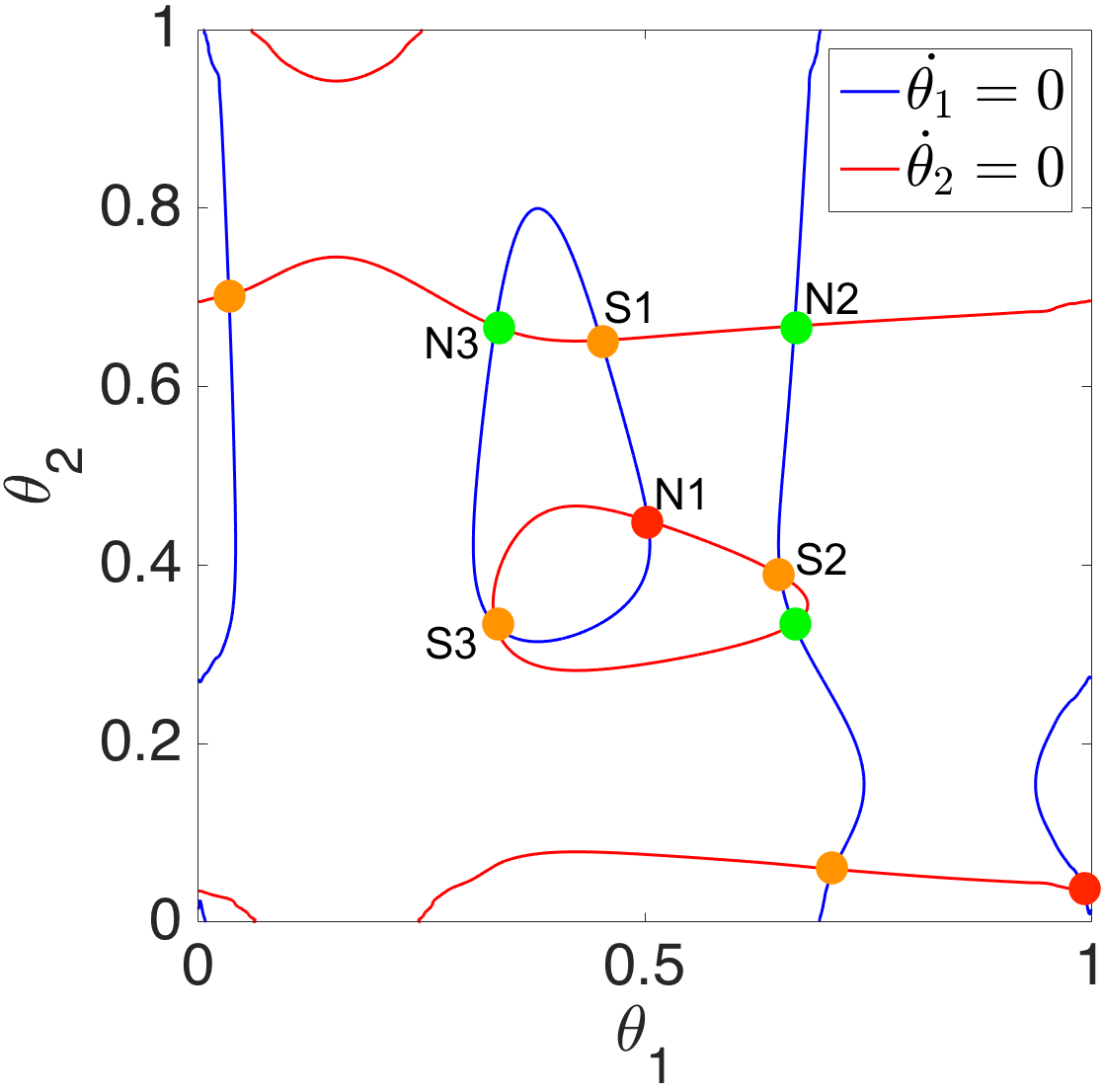
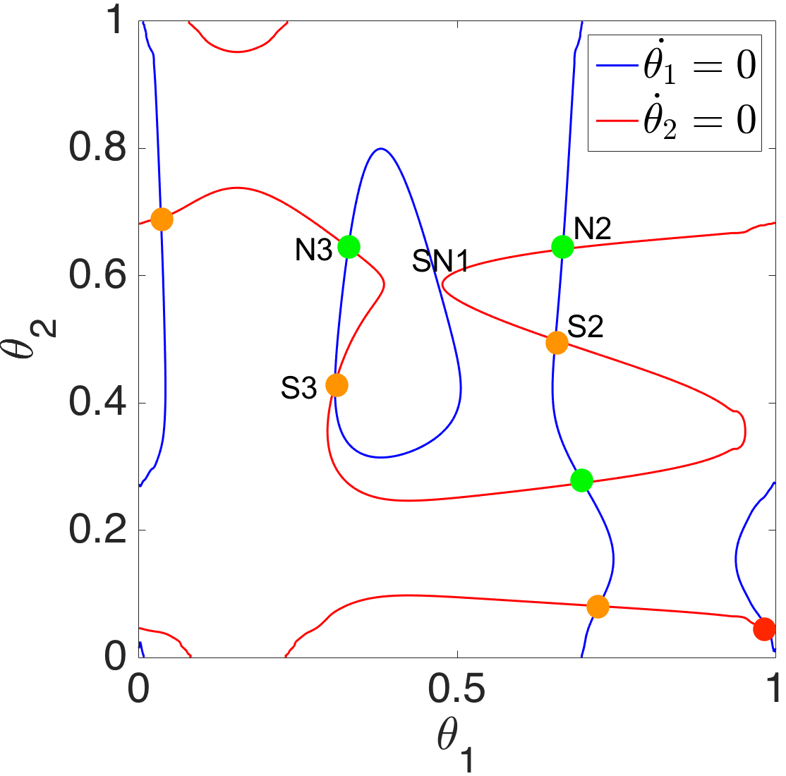
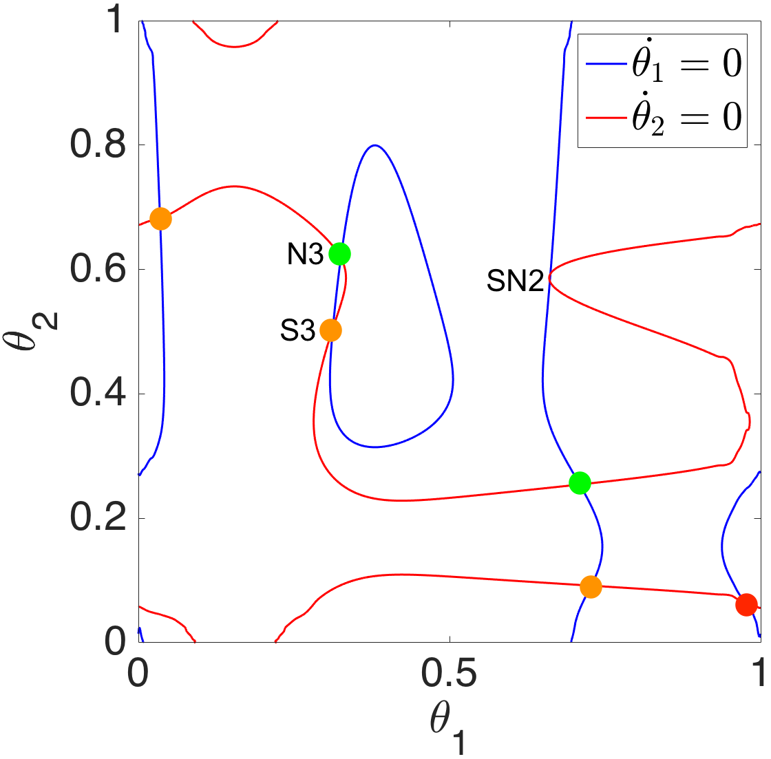
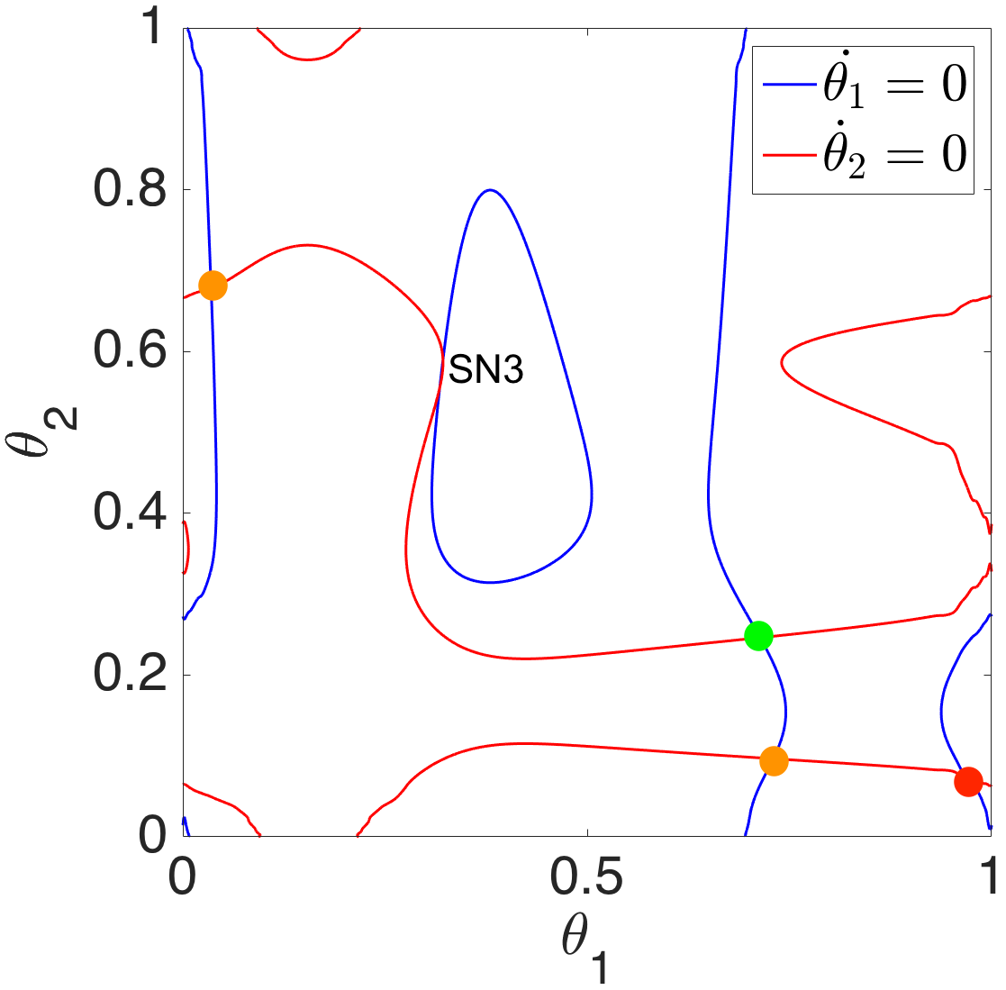
Figure 4: (Left to right) Nullclines of Equations (25) when ${c}_{i}$’s satisfy Equation (26), $I_{ext}=35.65$, and $\delta I\approx 0,0.02,0.032,0.038$, respectively. $\dot{\theta}_{1}=0$ nullcline shown in blue; $\dot{\theta}_{2}=0$ nullcline shown in red. Green dots indicate sinks, red dots are sources, and orange dots are saddle points. At $\delta I\approx 0.02$, the first saddle-node bifurcation (shown by SN1) occurs and the unstable tripod gait (shown by N1) disappears together with a saddle point (shown by S1). At $\delta I\approx 0.032$, the second saddle-node bifurcation (shown by SN2) occurs and a stable fixed point (shown by N2) disappears together with a saddle point (shown by S2). Finally, at $\delta I\approx 0.038$, the third saddle-node bifurcation (shown by SN3) occurs and the stable backward tetrapod gait (shown by N3) disappears together with a saddle point (shown by S3). A single stable approximate forward tetrapod gait remains together with a source and two saddle points.

Note that the balance condition is sufficient for the existence of forward and backward tetrapod gaits but does not guarantee their stability. Assuming that the balance condition holds, in [1, Proposition 6 (resp. Proposition 7)] we proved that the forward (resp. backward) tetrapod gait is always stable if ${c}_{1}={c}_{2}={c}_{3}$, and $\alpha:=\frac{c_{4}}{c_{4}+c_{7}}<\alpha_{max}$ (resp. $\alpha>\alpha_{min}$), where $\alpha_{max}$ (resp. $\alpha_{min}$) can be computed from the derivatives of $H$:

$$\alpha_{max}({\xi}):=\frac{H^{\prime}\left(\frac{1}{3};{\xi}\right)}{H^{\prime}\left(\frac{1}{3};{\xi}\right)-H^{\prime}\left(\frac{2}{3};{\xi}\right)},\quad\alpha_{min}({\xi}):=\frac{H^{\prime}\left(\frac{2}{3};{\xi}\right)}{H^{\prime}\left(\frac{2}{3};{\xi}\right)-H^{\prime}\left(\frac{1}{3};{\xi}\right)}.$$ (27)

Recall that here we fixed the speed parameter ${\xi}=I_{ext}$, so $\alpha_{max}$ and $\alpha_{min}$ are constant.

Without loss of generality, we can assume that one of the coupling strengths is equal to 1. For the rest of the paper we assume that ${c}_{4}=1$, the balance condition (22) holds, and ${c}_{1}={c}_{2}={c}_{3}$. Therefore, by making a change of time variable that eliminates ${c}_{5}={c}_{6}=1+{c}_{7}=1/\alpha$, Equations (25) can be written as

$$\dot{\theta}_{1}=\alpha(\tilde{\omega}_{1}-\tilde{\omega}_{2})+H(-\theta_{1};{\xi})-\alpha H(\theta_{1};{\xi})-(1-\alpha)H(\theta_{2};{\xi}),$$ (28a)

$$\dot{\theta}_{2}=\alpha(\tilde{\omega}_{3}-\tilde{\omega}_{2})+H(-\theta_{2};{\xi})-\alpha H(\theta_{1};{\xi})-(1-\alpha)H(\theta_{2};{\xi}),$$ (28b)

which possess both forward and backward tetrapod gaits with stabilities dependent on the value of ${\alpha}$, i.e., for

• ${\alpha}<{\alpha}_{min}$, the forward tetrapod gait is stable while the backward tetrapod gait is a saddle;

• ${\alpha}_{min}<{\alpha}<{\alpha}_{max}$, both backward and forward tetrapod gaits are stable;

• ${\alpha}>{\alpha}_{max}$, the backward tetrapod gait is stable while the forward tetrapod gait is a saddle.

In Sections 5.1 and 5.2, we do the following.

Section 5.1

We assume ${\alpha}<{\alpha}_{max}$ and let $\delta I_{f}\;:=\;I_{ext}^{1}(t)=I_{ext}^{2}(t)\;\geq\;0,$ and $I_{ext}^{3}(t)=0$. We show that for some small value of the heterogeneity parameter $\delta I_{f}$, Equations (28) possess only one stable forward tetrapod gait (together with a source and 2 saddle points).

Section 5.2

We assume ${\alpha}>{\alpha}_{min}$ and let $\delta I_{b}\;:=\;I_{ext}^{2}(t)=I_{ext}^{3}(t)\;\geq\;0,$ and $I_{ext}^{1}(t)=0$. We show that for some small value of the heterogeneity parameter $\delta I_{b}$, Equations (28) possess only one stable backward tetrapod gait (together with a source and 2 saddle points).

5.1 Emergence of a unique stable forward tetrapod gait at low speed

We assume ${\alpha}<{\alpha}_{max}$ so that the forward tetrapod gait, $(2/3,1/3)$, is stable while the backward tetrapod gait can be either stable or a saddle, as described above. For any $t$, let

$$\delta I_{f}\;:=\;I_{ext}^{1}(t)=I_{ext}^{2}(t)\;\geq\;0,\quad I_{ext}^{3}(t)=0,$$ (29)

and consider the heterogeneity parameter $\delta I_{f}$ as a bifurcation parameter.

Choosing ${I_{ext}^{i}(t)}$ as in Equation (29) implies $\tilde{\omega}_{1}-\tilde{\omega}_{2}=0$, and $\tilde{\omega}_{3}-\tilde{\omega}_{2}=-\delta I_{f}\bar{Z}\leq 0$, where $\bar{Z}=\frac{1}{T}\int_{0}^{T}Z_{v}(\Gamma(t))\;dt>0$ is the average of the phase response curve. Therefore, Equations (28) become

$$\dot{\theta}_{1}=H(-\theta_{1};{\xi})-\alpha H(\theta_{1};{\xi})-(1-\alpha)H(\theta_{2};{\xi}),$$ (30a)

$$\dot{\theta}_{2}=-\alpha\delta I_{f}\bar{Z}+H(-\theta_{2};{\xi})-\alpha H(\theta_{1};{\xi})-(1-\alpha)H(\theta_{2};{\xi}).$$ (30b)

Equations (30) can also be obtained if $I_{ext}^{1}(t)=I_{ext}^{2}(t)=0,\;\delta I_{f}=I_{ext}^{3}(t)<0.$

We will show that when $\alpha_{min}<\alpha<\alpha_{max}$ (resp. $0<\alpha<\alpha_{min}$), as the bifurcation parameter $\delta I_{f}$ increases, Equations (30) lose 6 (resp. 4) fixed points through 3 (resp. 2) saddle-node bifurcations and keep only one stable approximate forward tetrapod gait. To show this, we consider two topologically different cases:

$\alpha_{min}<\alpha<\alpha_{max}$

At $\delta I_{f}=0$, Equations (30) admit 10 fixed points (5 saddle points, 3 sinks, and 2 sources). As $\delta I_{f}$ increases, 3 saddle-node bifurcations occur and one sink (corresponding to the approximate forward tetrapod gait), one source and 2 saddle points remain.

$0<\alpha<\alpha_{min}$

At $\delta I_{f}=0$, Equations (30) admit 8 fixed points (4 saddle points, 2 sinks, and 2 sources). As $\delta I_{f}$ increases, 2 saddle-node bifurcations occur and one sink (corresponding to the approximate forward tetrapod gait), one source and 2 saddle points remain.

Figure 5 shows that as ${\alpha}$ decreases and approaches ${\alpha}_{min}$, through a saddle-node bifurcation the stable backward tetrapod gait disappears and one of the saddle points moves toward the position of the backward tetrapod gait, which is shown by an arrow in Figure 5 (left). As $\alpha$ decreases, the isolated $\dot{\theta}_{1}=0$ nullcline combines with the $\dot{\theta}_{1}=0$ nullcline that encircles the torus and thereafter the number of fixed points reduces to 8 from 10. Therefore, when $0<{\alpha}<{\alpha}_{min}$, there are only 8 fixed points.

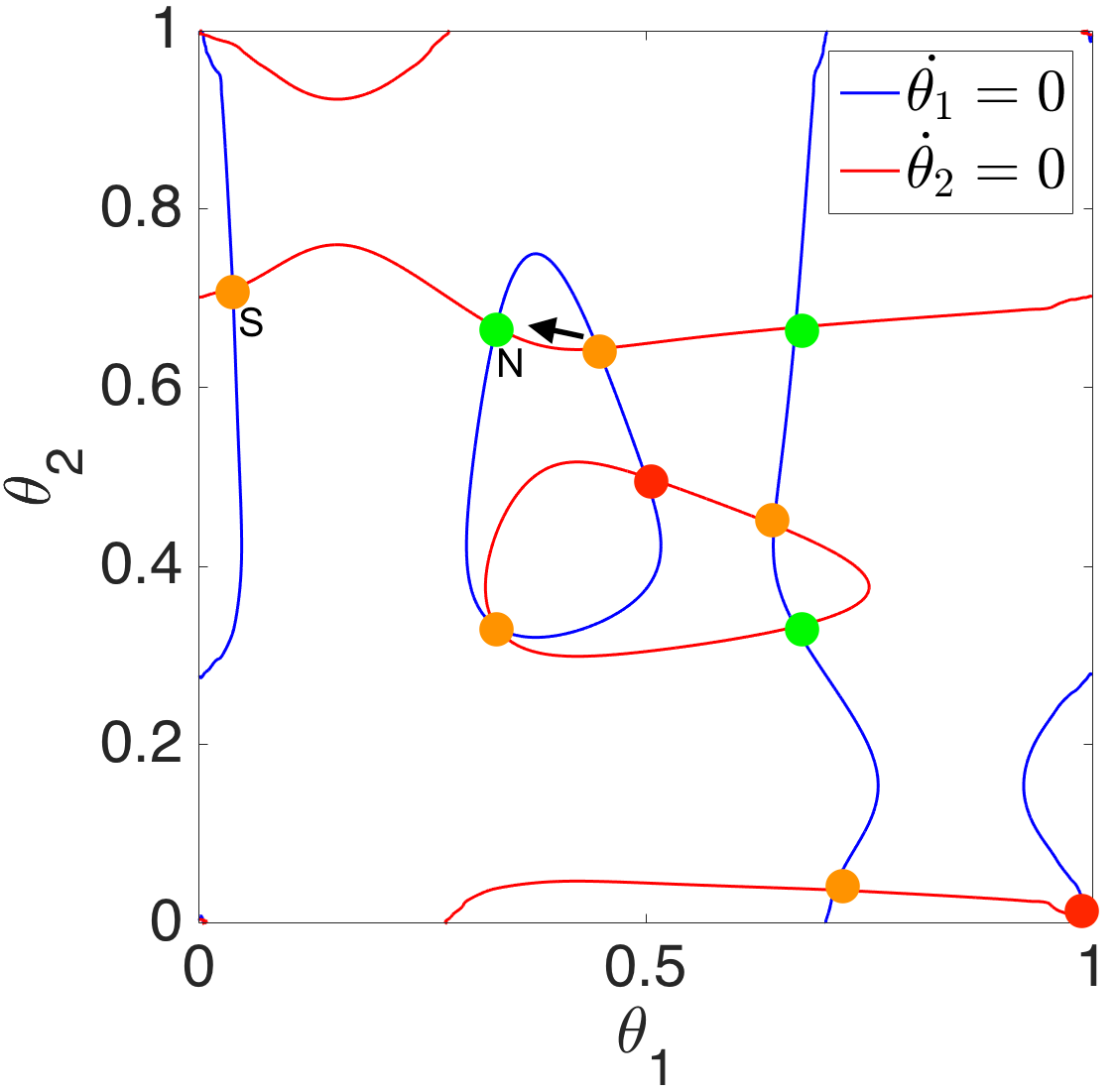
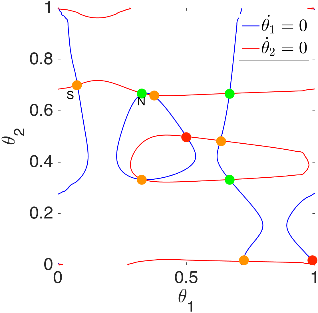
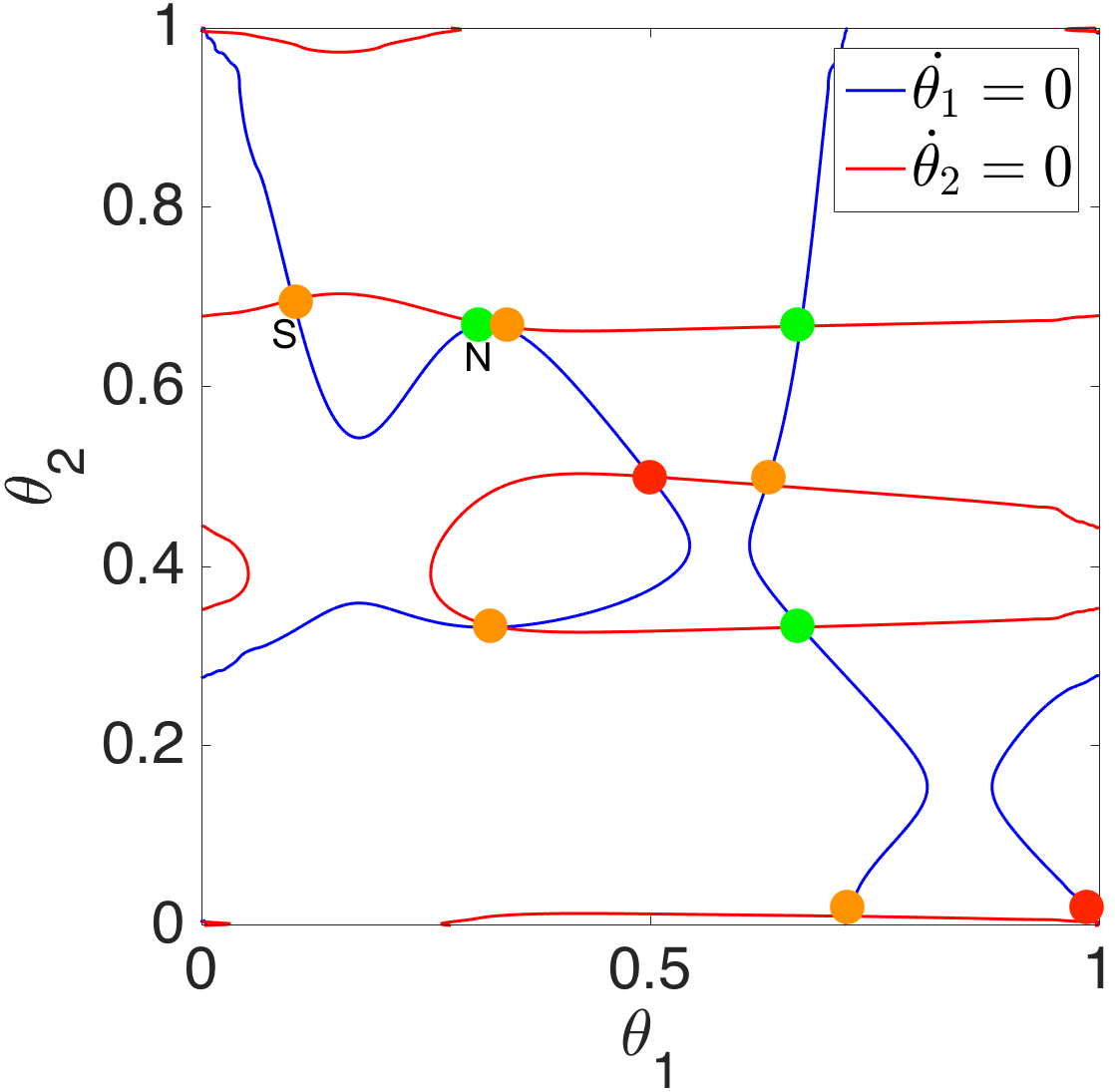
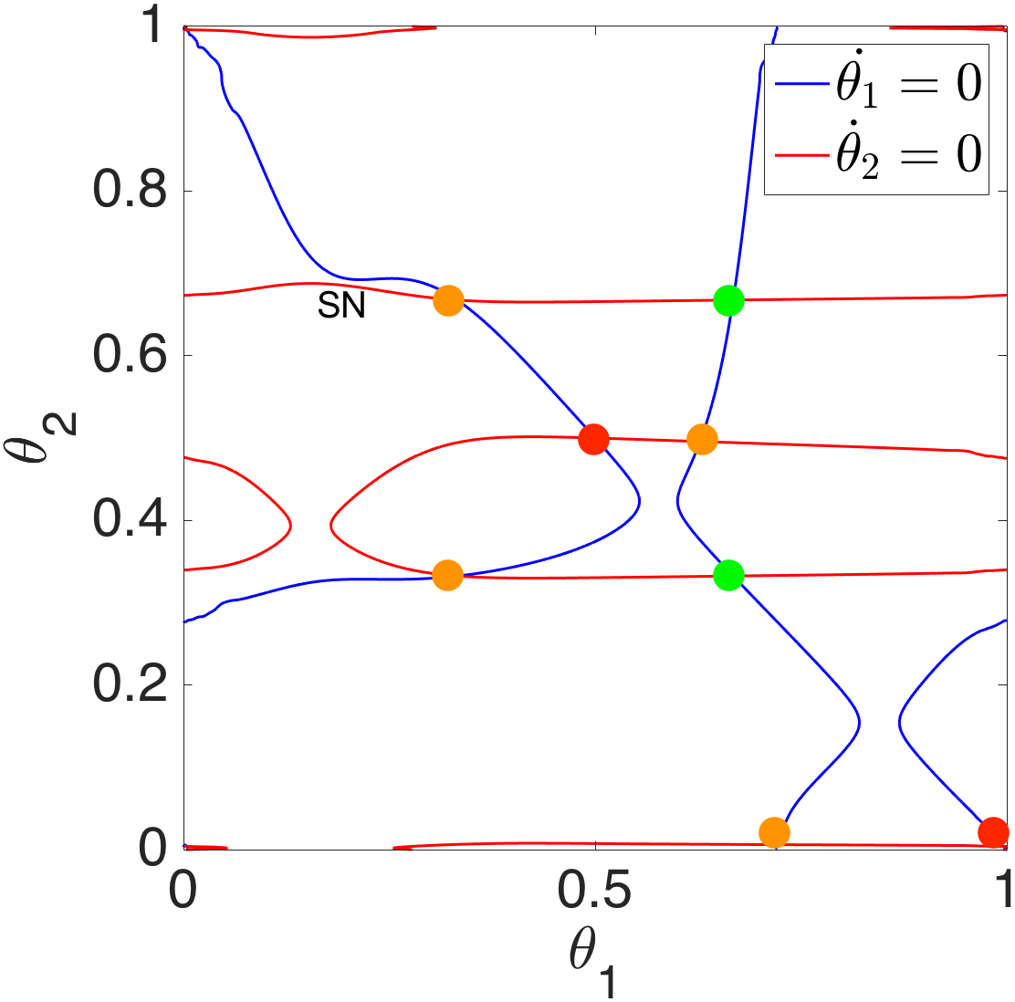
Figure 5: (Left to right) Nullclines of Equations (30) with $\alpha=1/2,1/5,1/8,1/17$, $I_{ext}=35.65$, and $\delta I_{f}=0$, respectively. At $\alpha=1/2$, there exist 10 fixed points including one stable backward tetrapod gait shown by N. As $\alpha$ decreases, through a saddle-node bifurcation (shown by SN) the stable backward tetrapod gait disappears together with a saddle point shown by S and another saddle point becomes a backward tetrapod gait. Nullclines and fixed points are indicated as in Figure 4.

3 saddle-node bifurcations: $\alpha_{min}<\alpha<\alpha_{max}$

Consider Equations (30) with $\alpha_{min}<\alpha<\alpha_{max}$. Since the qualitative behavior of the solutions of Equations (30) with $\alpha_{min}<\alpha<\alpha_{max}$ are all similar, we show the results in an example with ${\alpha}=1/2$. As is clear from Equations (30) and illustrated in Figure 6, choosing the heterogeneity of Equation (29) maintains the $\dot{\theta}_{1}=0$ nullclines and only perturbs the $\dot{\theta}_{2}=0$ nullclines. This perturbation causes the topology of the $\dot{\theta}_{2}=0$ nullclines to change, combining the isolated closed curve of the $\dot{\theta}_{2}=0$ nullcline with a nullcline that encircles the torus and thereafter reducing the number of fixed points. In this case, where $\alpha=1/2$, at $\delta I_{f}=0$, there exist 3 stable sinks, 2 unstable sources and 5 saddle points. As $\delta I_{f}$ increases, 3 saddle-node bifurcations occur at approximately $\delta I_{f}\approx 0.011,0.025,0.037$ and one stable fixed point remains, which corresponds to a stable approximate forward tetrapod gait. The other 3 remaining fixed points are a source and 2 saddle points.

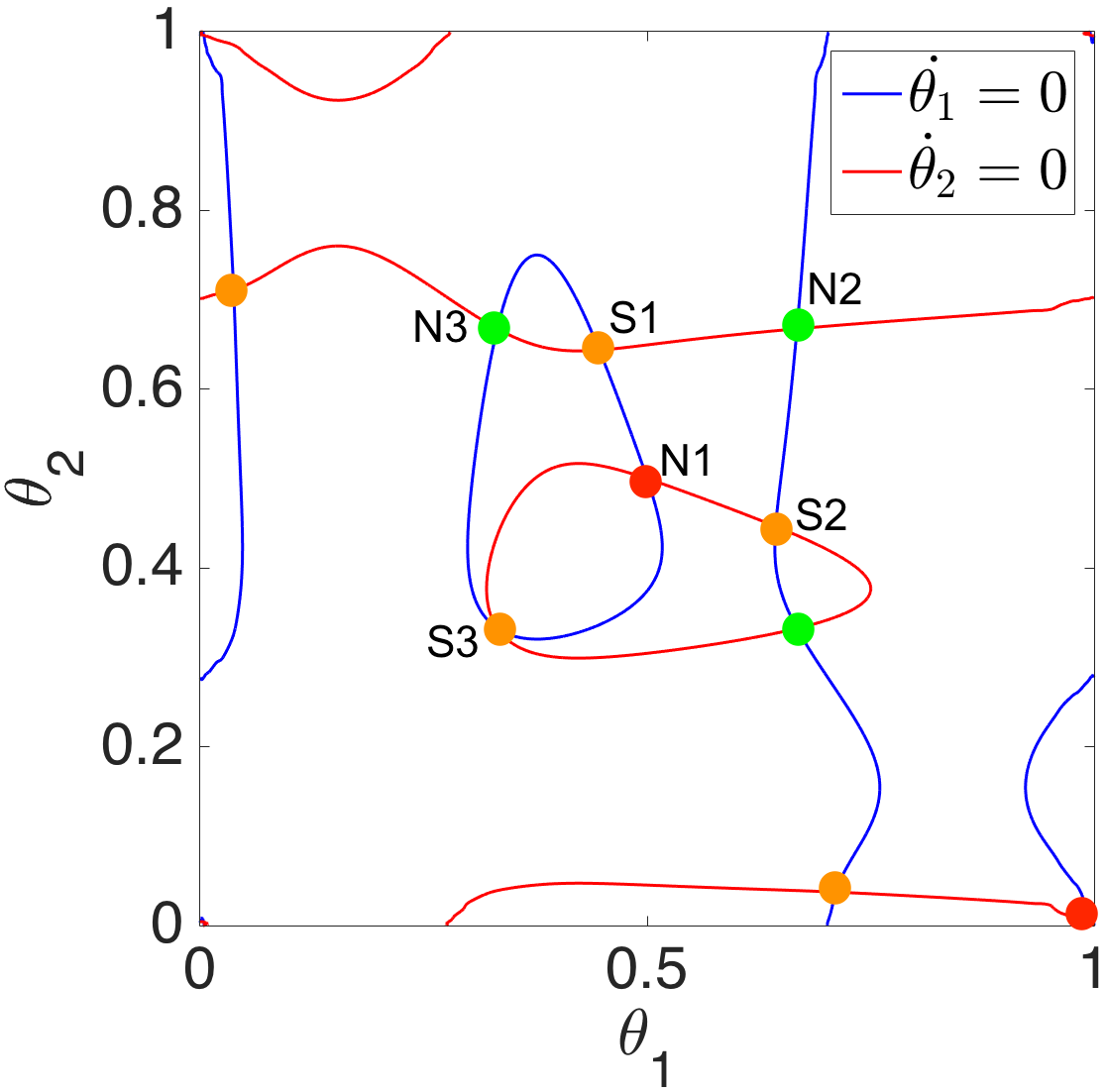
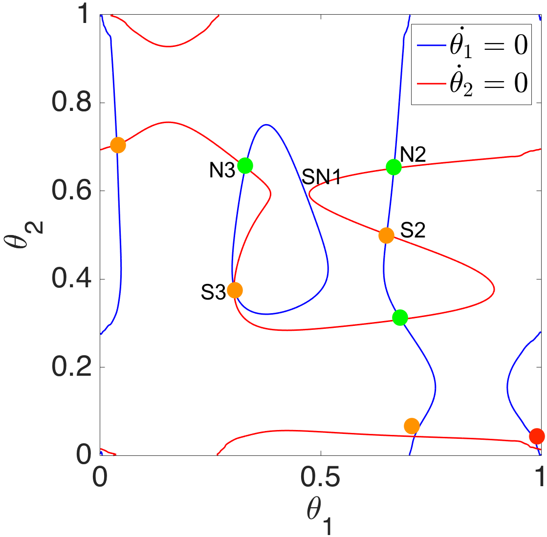
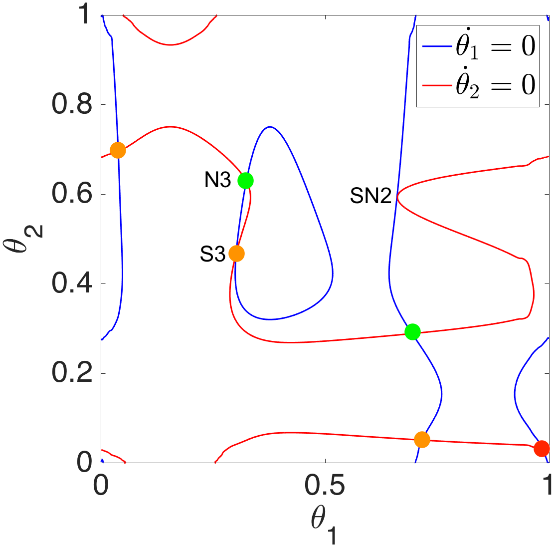
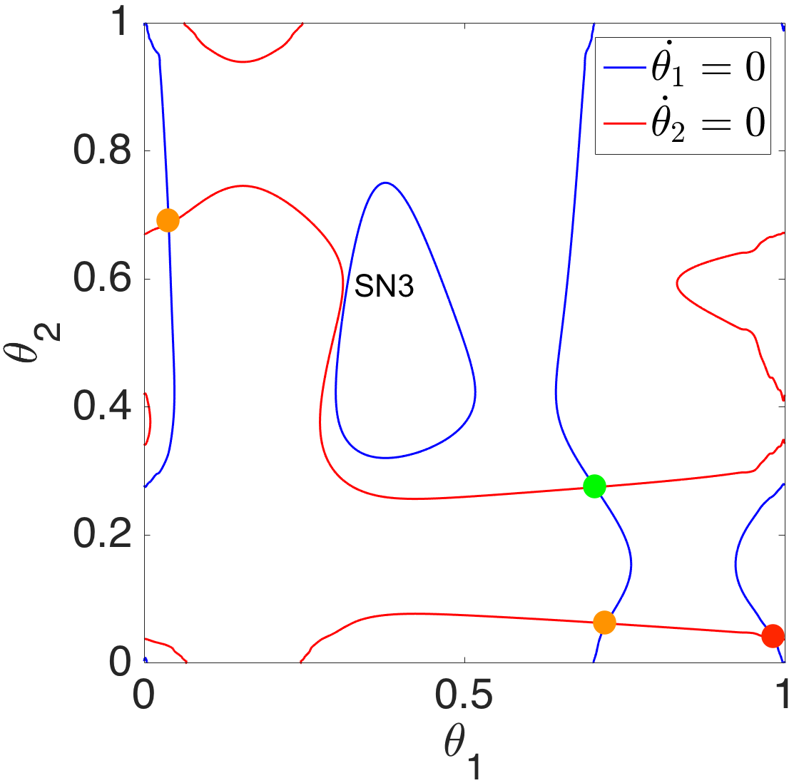
Figure 6: (Left to right) Nullclines of Equations (28) with $\alpha=1/2$, $I_{ext}=35.65$, and $\delta I_{f}\approx 0,0.011,0.025,0.037$, respectively. At $\delta I_{f}=0$, there exist ten fixed points. At $\delta I_{f}\approx 0.011$, the first saddle-node bifurcation (shown by SN1) occurs and the unstable tripod gait (shown by N1) disappears together with a saddle point (shown by S1). At $\delta I_{f}\approx 0.025$, the second saddle-node bifurcation (shown by SN2) occurs and a stable fixed point (shown by N2) disappears together with a saddle point (shown by S2). Finally, at $\delta I_{f}\approx 0.037$, the third saddle-node bifurcation (shown by SN3) occurs and the stable backward tetrapod gait (shown by N3) disappears together with a saddle point (shown by S3). A single stable approximate forward tetrapod gait remains together with a source and two saddle points. Nullclines and fixed points are indicated as in Figure 4.

2 saddle-node bifurcations: $0<\alpha<\alpha_{min}$

We now consider Equations (30) with $\alpha<\alpha_{min}$. Since the qualitative behavior of the solutions of Equations (30) with $0<\alpha<\alpha_{min}$ are all similar, we only show the results for $\alpha\approx 0.03$. As illustrated in Figure 7, choosing the heterogeneity of Equation (29) maintains the $\dot{\theta}_{1}=0$ nullclines and, by combining two nullclines that encircle the torus, changes the topology of the $\dot{\theta}_{2}=0$ nullclines and thereafter, through two saddle-node bifurcations, reduces the number of fixed points. As $\delta I_{f}$ increases from 0 to $0.03$, one saddle-node bifurcation occurs in which the unstable tripod gait and the backward tetrapod gait disappear; as $\delta I_{f}$ increases further to $0.032$, another saddle-node bifurcation occurs and the stable fixed point on $\theta_{1}=\theta_{2}$ disappears and a unique stable approximate forward tetrapod gait remains at $(0.69,0.31)$. The nullclines at $\delta I_{f}\approx 0.029$ are shown to illustrate how the nullclines move toward each other and cause the saddle-node bifurcations.

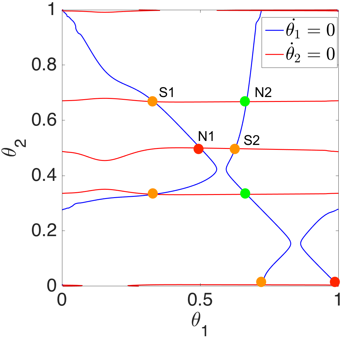
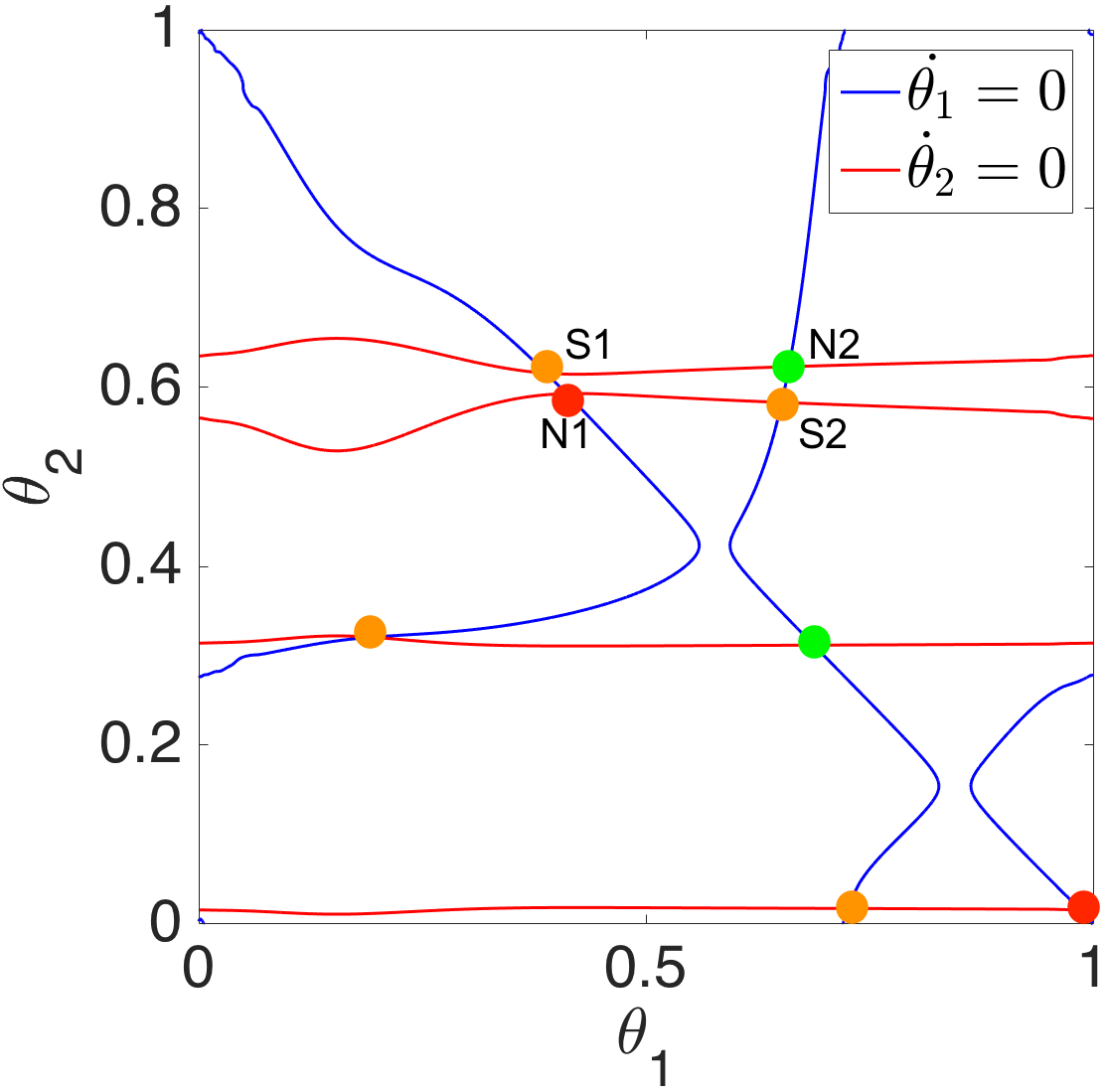
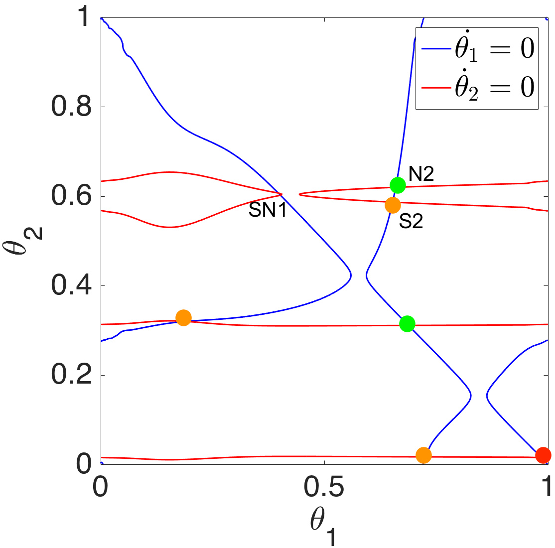
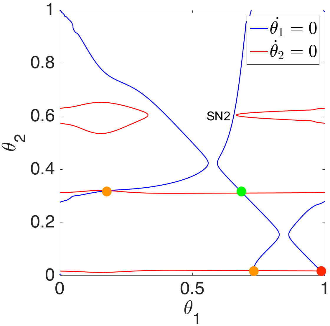
Figure 7: (Left to right) Nullclines of Equations (28) with $\alpha\approx 0.03$ , $I_{ext}=35.65$, and $\delta I_{f}\approx 0,0.029,0.03,0.032$, respectively. At $\delta I_{f}=0$, there exist one stable forward tetrapod gait, one unstable (saddle) backward tetrapod gait, and one unstable tripod gait. One stable fixed point on $\theta_{1}=\theta_{2}$ and several saddle points exist. At $\delta I_{f}\approx 0.03$, through a saddle-node bifurcation (shown by SN1), the unstable tripod gait (shown by N1) and the unstable backward tetrapod gait (shown by S1) disappear. At $\delta I_{f}\approx 0.032$, through another saddle-node bifurcation (shown by SN2), a stable fixed point (shown by N2) and a saddle point (shown by S2) disappear. A single stable approximate forward tetrapod gait remains, together with a source and two saddle points. Nullclines and fixed points are indicated as in Figure 4. Note that the second figure only shows how the nullclines move and it is topologically equivalent to the first figure.

So far, we assumed that the forward tetrapod gait is always stable and chose the control parameters ${I_{ext}^{i}(t)}$ to get a unique stable approximate forward tetrapod gait. In the following section, we assume that the backward tetrapod gait is always stable and show how to choose ${I_{ext}^{i}(t)}$ to get a unique stable approximate backward tetrapod gait. As discussed earlier, when ${\alpha}_{min}<{\alpha}$, the backward tetrapod gait is always stable.

5.2 Emergence of a unique backward tetrapod gait at low speed

We assume ${\alpha}_{min}<{\alpha}$ so that the backward tetrapod gait, $(1/3,2/3)$, is stable while the forward tetrapod gait can be either stable or a saddle.

For any $t$, let

$$\delta I_{b}\;:=\;I_{ext}^{2}(t)=I_{ext}^{3}(t)\;\geq\;0,\quad I_{ext}^{1}(t)=0,$$ (31)

and consider $\delta I_{b}$ as a bifurcation parameter.

Choosing ${I_{ext}^{i}(t)}$ as in Equation (31) implies $\tilde{\omega}_{3}-\tilde{\omega}_{2}=0$, and $\tilde{\omega}_{1}-\tilde{\omega}_{2}=-\delta I_{b}\bar{Z}\leq 0$. Therefore, Equations (28) become

$$\dot{\theta}_{1}=-\alpha\delta I_{b}\bar{Z}+H(-\theta_{1};{\xi})-\alpha H(\theta_{1};{\xi})-(1-\alpha)H(\theta_{2};{\xi}),$$ (32a)

$$\dot{\theta}_{2}=H(-\theta_{2};{\xi})-\alpha H(\theta_{1};{\xi})-(1-\alpha)H(\theta_{2};{\xi}).$$ (32b)

We will show that when $\alpha_{min}<\alpha<\alpha_{max}$ (resp. $\alpha>\alpha_{max}$), as the bifurcation parameter $\delta I_{b}$ increases, Equations (32) lose 6 (resp. 4) fixed points through 3 (resp. 2) saddle-node bifurcations and keep only one stable approximate backward tetrapod gait. To show this, we consider two topologically different cases:

$\alpha_{min}<\alpha<\alpha_{max}$

At $\delta I_{b}=0$, Equations (32) admit 10 fixed points (5 saddle points, 3 sinks, and 2 sources). As $\delta I_{b}$ increases, 3 saddle-node bifurcations occur and one sink (corresponding to the approximate backward tetrapod gait), one source and 2 saddle points remain.

$\alpha>\alpha_{max}$

At $\delta I_{b}=0$, Equations (32) admit 8 fixed points (4 saddle points, 2 sinks, and 2 sources). As $\delta I_{b}$ increases, 2 saddle-node bifurcations occur and one sink (corresponding to the approximate backward tetrapod gait), one source and 2 saddle points remain.

Figure 8 shows that as ${\alpha}$ increases and approaches ${\alpha}_{max}$, through a saddle-node bifurcation, the stable forward tetrapod gait disappears and one of the saddle points moves toward the position of the forward tetrapod gait, as shown by an arrow in Figure 8 (left). As $\alpha$ increases, the isolated $\dot{\theta}_{2}=0$ nullcine combines with the $\dot{\theta}_{2}=0$ nullcline that encircles the torus and thereafter, at ${\alpha}={\alpha}_{max}$, the number of fixed points reduces to 8 from 10. Therefore, when ${\alpha}>{\alpha}_{max}$, there are only 8 fixed points.

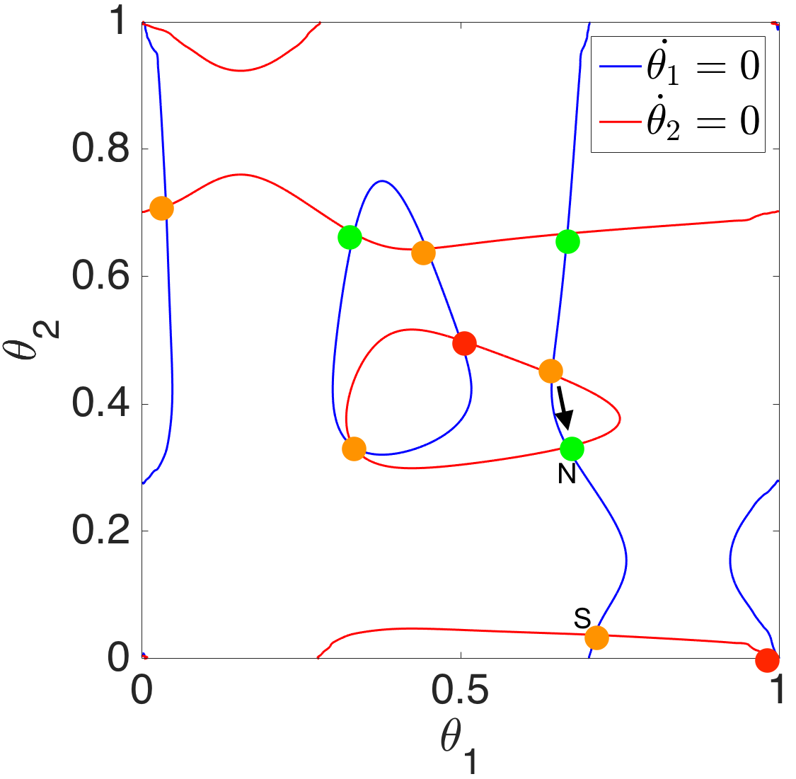
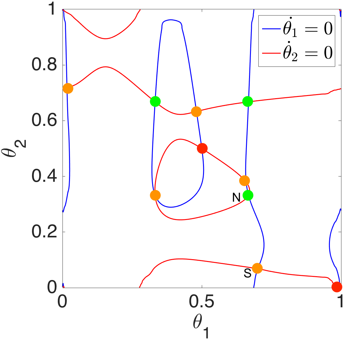
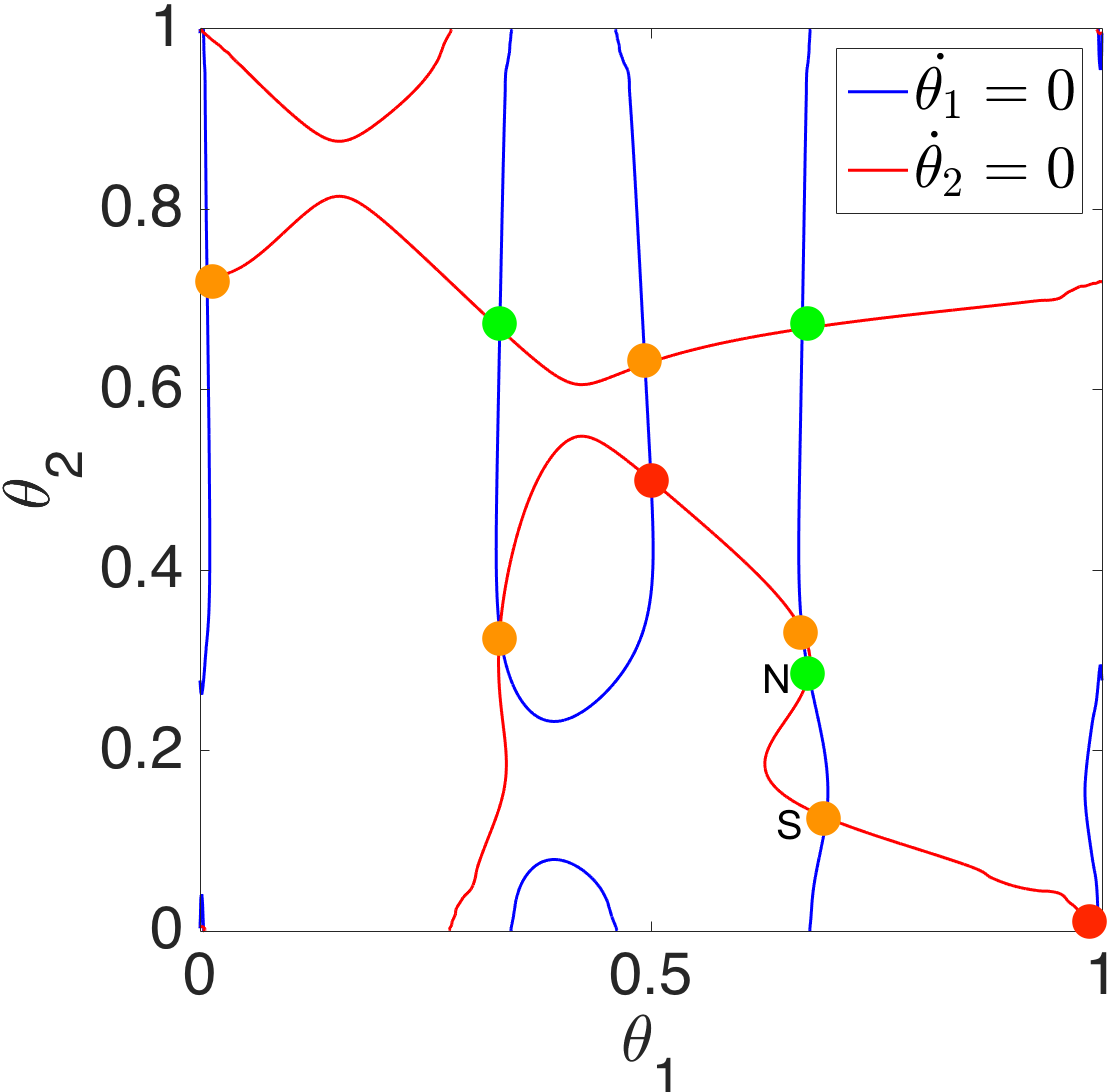
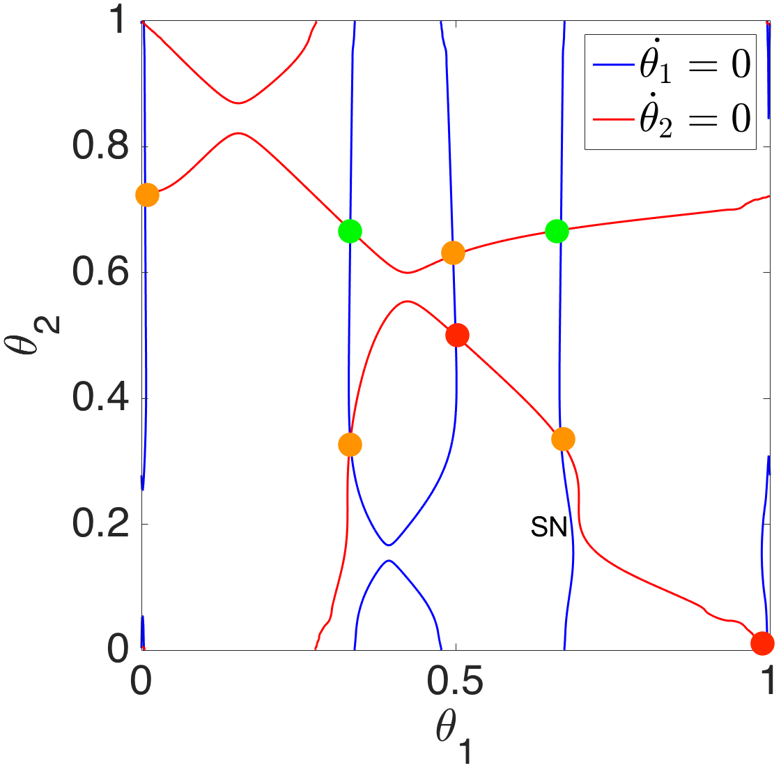
Figure 8: (Left to right) Nullclines of Equations (32) with $\alpha=1/2,1/1.3,1/1.1,1/1.06$, $I_{ext}=35.65$, and $\delta I_{b}=0$, respectively. At $\alpha=1/2$, there exist 10 fixed points including one stable forward tetrapod gait shown by N. As $\alpha$ increases, through a saddle-node bifurcation (shown by SN) the stable forward tetrapod gait disappears together with a saddle point shown by S and another saddle point becomes an unstable forward tetrapod gait. The stable backward tetrapod remains throughout. Nullclines and fixed points are indicated as in Figure 4.

3 saddle-node bifurcations: $\alpha_{min}<\alpha<\alpha_{max}$

Consider Equations (32) with $\alpha_{min}<\alpha<\alpha_{max}$. Since the qualitative behavior of the solutions of Equations (32) with $\alpha_{min}<\alpha<\alpha_{max}$ are all similar, we show the results in an example with ${\alpha}=1/3$. As is clear from Equations (32) and illustrated in Figure 9, choosing the heterogeneity of Equation (31), maintains the $\dot{\theta}_{2}=0$ nullclines and only perturbs the $\dot{\theta}_{1}=0$ nullclines. This perturbation causes the topology of the $\dot{\theta}_{1}=0$ nullclines to change, combining the isolated circle with a nullcline that encircles the torus and thereafter reducing the number of fixed points.

In Figure 9, we show the nullclines of Equations (32) with $\alpha=1/3$, and increase $\delta I_{b}$ from 0 to $0.015$, where the first saddle-node bifurcation occurs and the unstable tripod gait disappears. We further increase $\delta I_{b}$ to $0.04$ where the second saddle-node bifurcation occurs and the stable $\approx(2/3,2/3)$ fixed point disappears. Finally, when $\delta I_{b}$ reaches $0.056$, the third saddle-node bifurcation occurs and the stable forward tetrapod gait disappears and only one stable fixed point remains, which corresponds to the approximate backward tetrapod gait $\approx(0.25,0.7)$, as we desired.

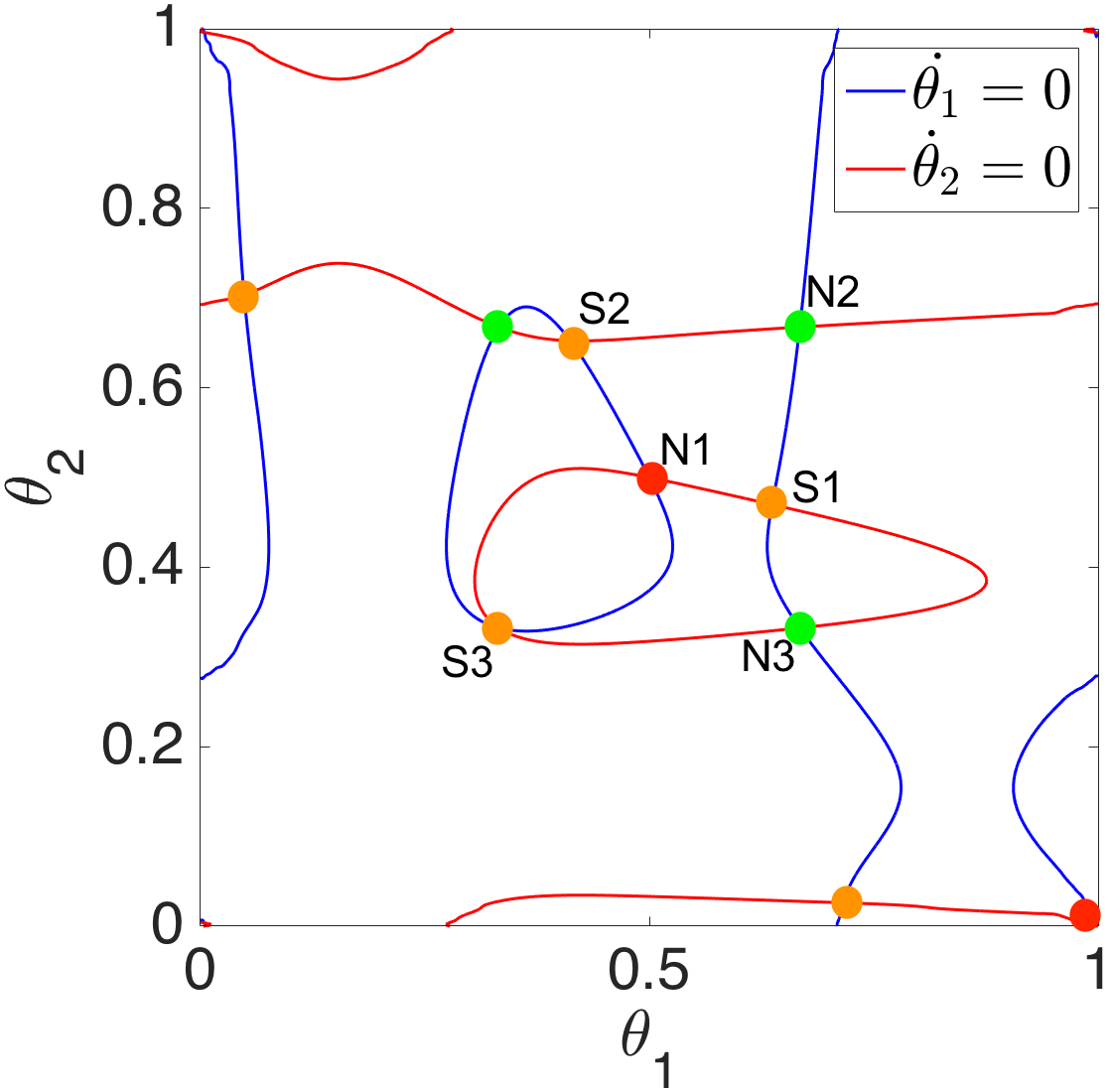
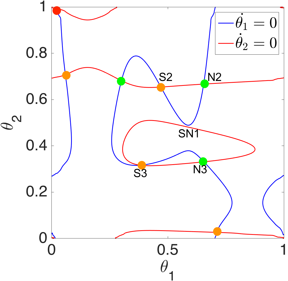
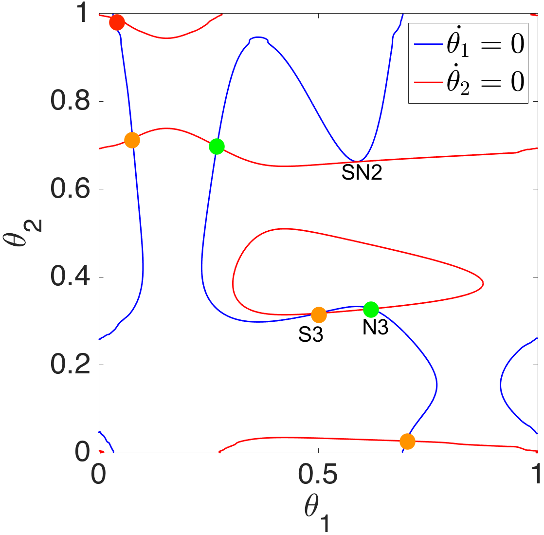
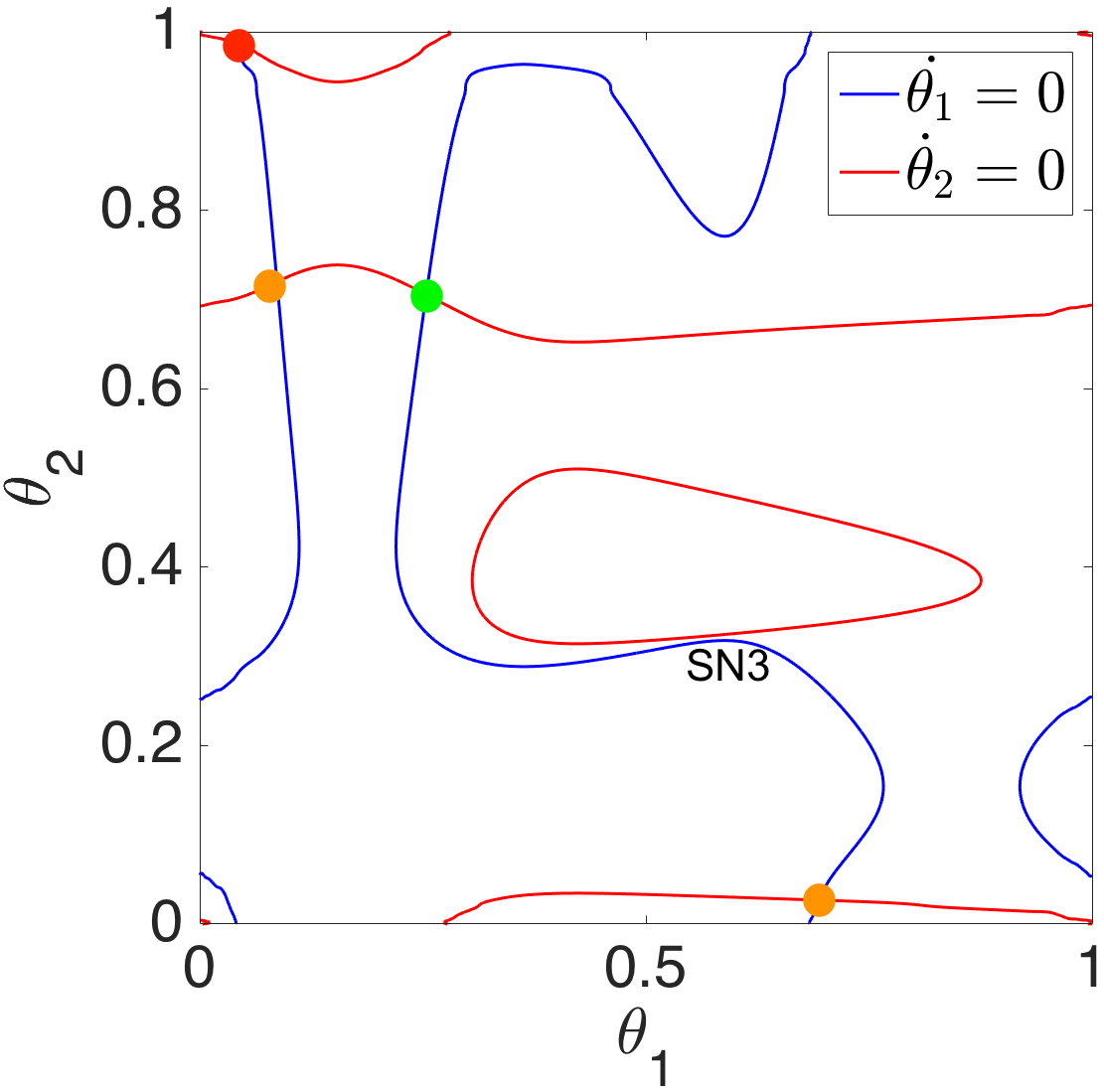
Figure 9: (Left to right) Nullclines of Equations (32) with $\alpha=1/3$, $I_{ext}=35.65$, and $\delta I_{b}\approx 0,0.015,0.04,0.056$, respectively. At $\delta I_{b}=0$, there exist ten fixed points. At $\delta I_{b}\approx 0.015$, the first saddle-node bifurcation (shown by SN1) occurs and the unstable tripod gait (shown by N1) disappears together with a saddle point (shown by S1). At $\delta I_{b}\approx 0.04$, the second saddle-node bifurcation (shown by SN2) occurs and a stable fixed point (shown by N2) disappears together with a saddle point (shown by S2). Finally, at $\delta I_{b}\approx 0.056$, the third saddle-node bifurcation (shown by SN3) occurs and the stable forward tetrapod gait (shown by N3) disappears together with a saddle point (shown by S3). A single stable approximate backward tetrapod gait remains, together with a source and two saddle points. Nullclines and fixed points are indicated as in Figure 4.

2 saddle-node bifurcations: $\alpha>\alpha_{max}$

We now consider Equations (32) with $\alpha>\alpha_{max}$. Since the qualitative behavior of the solutions of Equations (32) with $\alpha>\alpha_{max}$ are all similar, we only show the results for $\alpha\approx 0.95$. As is illustrated in Figure 10, choosing the heterogeneity of Equation (31) maintains the $\dot{\theta}_{2}=0$ nullclines and, by combining two $\dot{\theta}_{1}=0$ nullclines that encircle the torus, changes the topology of the $\dot{\theta}_{1}=0$ nullclines and thereafter, through two saddle-node bifurcations, reduces the number of fixed points. As $\delta I_{b}$ increases from 0 to $0.0121$, one saddle-node bifurcation occurs in which the unstable tripod gait and the backward tetrapod gait disappear; as $\delta I_{b}$ increases further to $0.013$, another saddle-node bifurcation occurs and the stable fixed point shown by N2 disappears and a unique stable approximate backward tetrapod gait remains at $(0.31,0.69)$. The nullclines at $\delta I_{b}\approx 0.012$ are shown to illustrate how the $\dot{\theta}_{1}=0$ nullclines move toward each other and cause the saddle-node bifurcations.

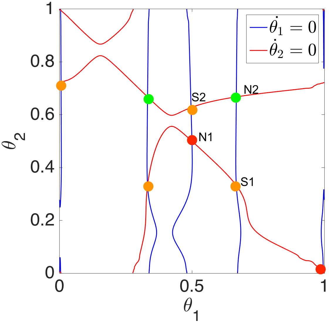
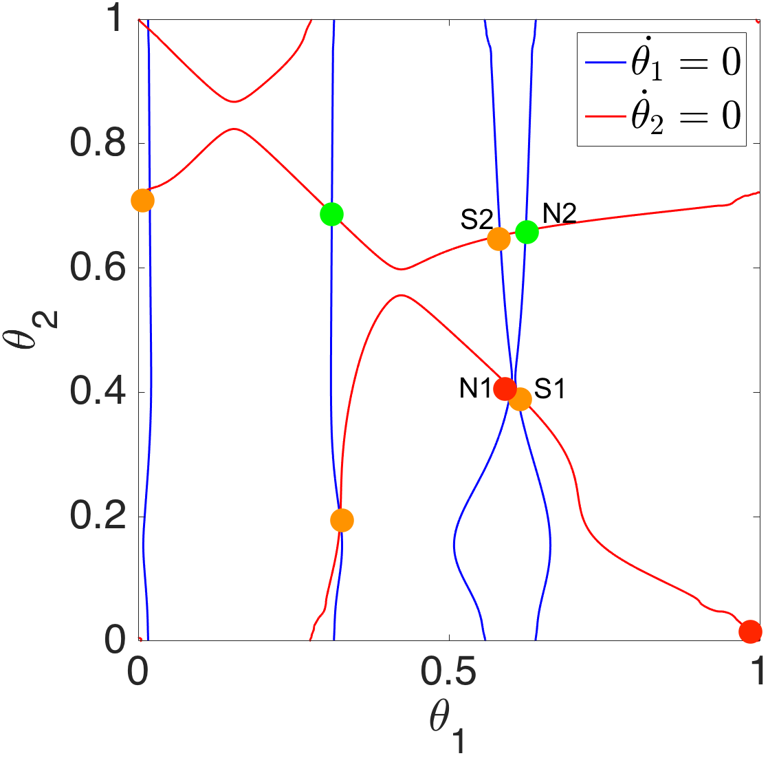
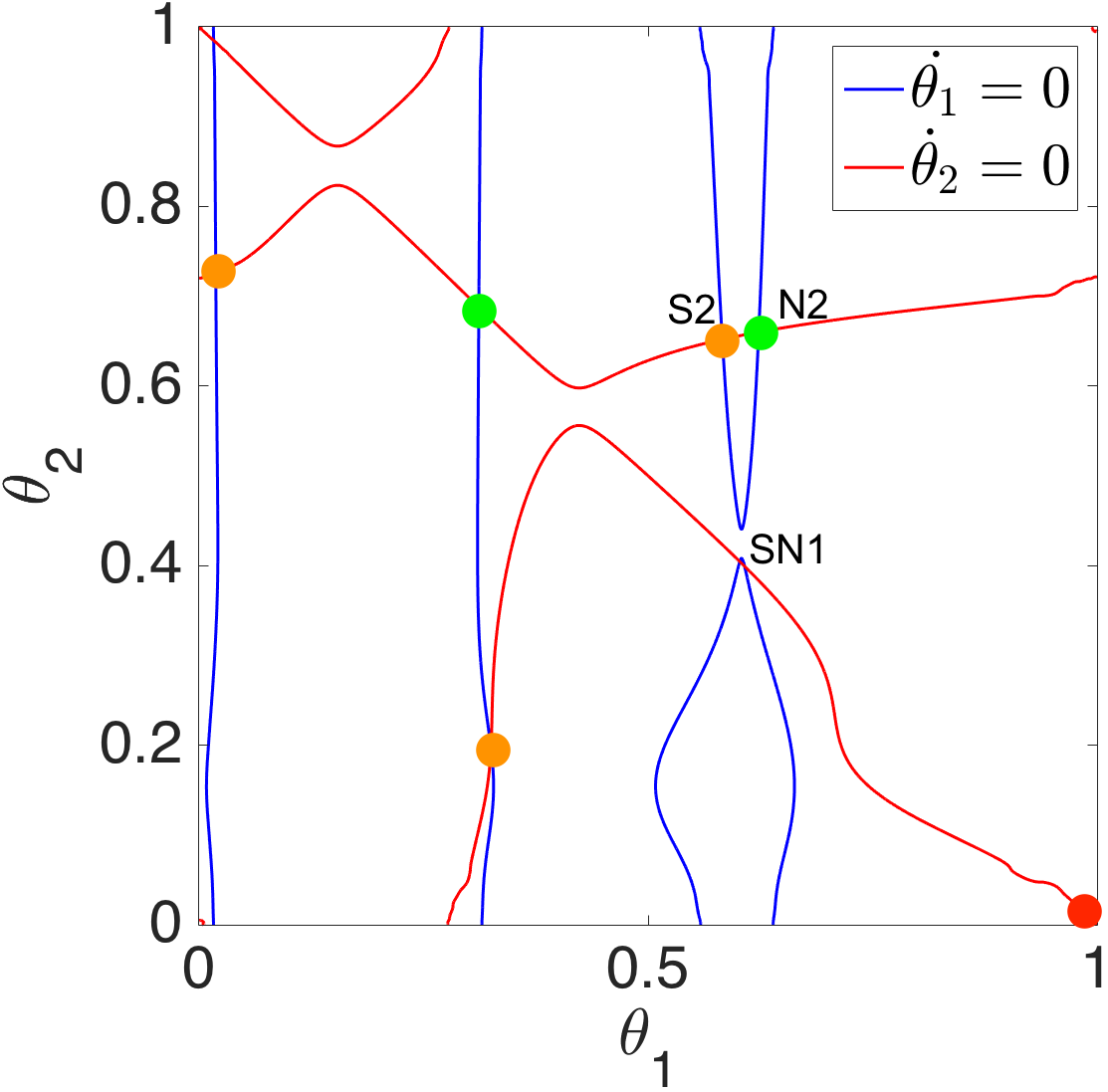
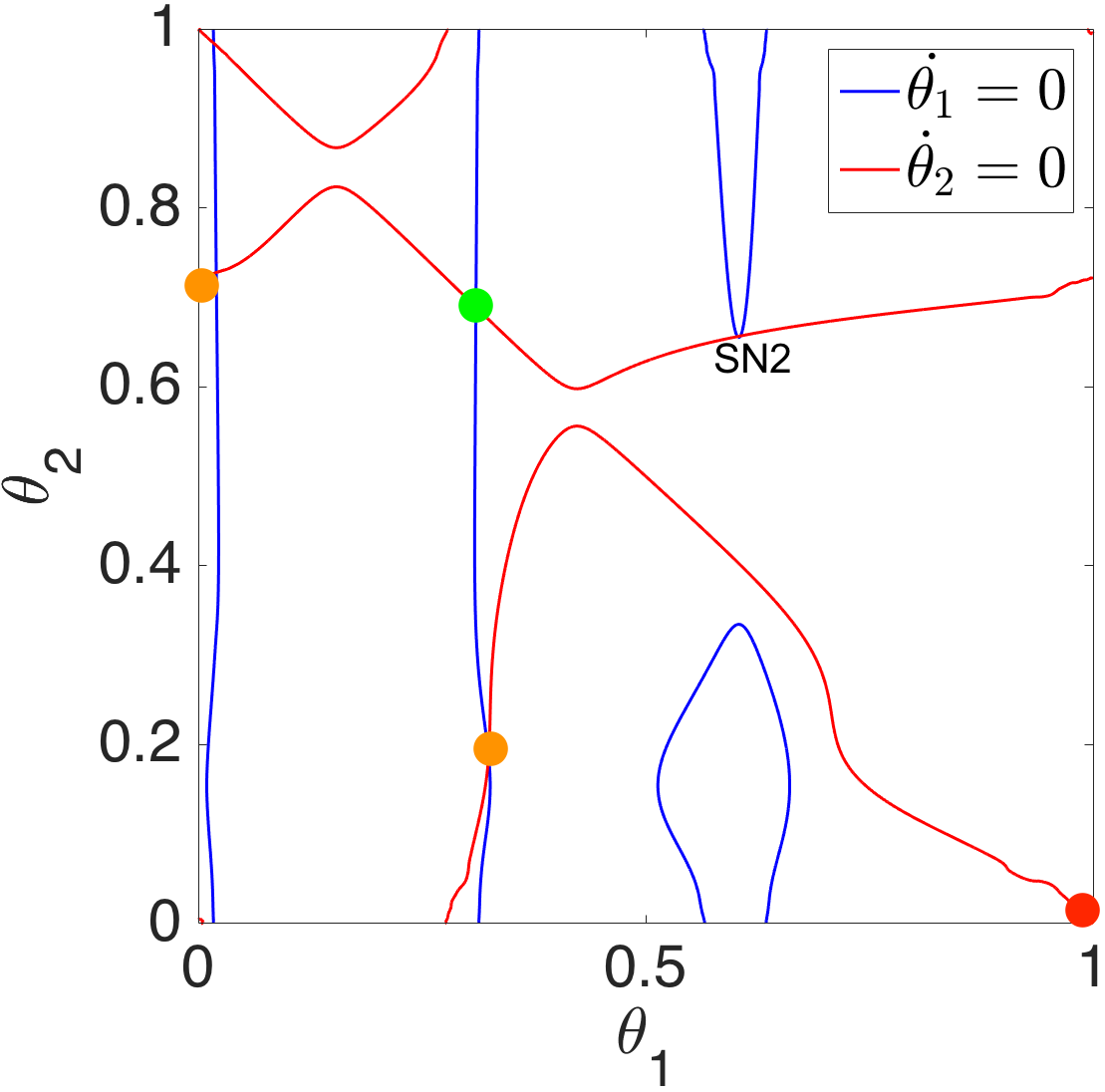
Figure 10: (Left to right) Nullclines of Equations (32) with $\alpha\approx 0.95$ , $I_{ext}=35.65$, and $\delta I_{b}\approx 0,0.012,0.0121,0.013$, respectively. At $\delta I_{b}=0$, there exist one stable backward tetrapod gait, one unstable (saddle) forward tetrapod gait, and one unstable tripod gait. One stable fixed point on $\theta_{1}=\theta_{2}$ and four saddle points exist. At $\delta I_{b}\approx 0.0121$, through a saddle-node bifurcation (shown by SN1), the unstable tripod gait (shown by N1) and the unstable forward tetrapod gait (shown by S1) disappear. At $\delta I_{b}\approx 0.013$, through another saddle-node bifurcation (shown by SN2), a stable fixed point (shown by N2) and a saddle point (shown by S2) disappear. A single stable approximate backward tetrapod gait remains together with a source and two saddle points. Nullclines and fixed points are indicated as in Figure 4. Note that the second panel only shows how the $\dot{\theta}_{1}=0$ nullclines move and it is topologically equivalent to the first panel.

Remark 1.

In Table 2, we summarize the main results shown in Figures 5–10.

Figure #	${\alpha}$	$I^{1}_{ext}$	$I^{2}_{ext}$	$I^{3}_{ext}$	bifurcation type
5	varies	0	0	0	1 saddle-node
6	${\alpha}_{min}<{\alpha}<{\alpha}_{max}$	($=\delta I_{f}$) varies	($=\delta I_{f}$) varies	0	3 saddle-node
7	$0<{\alpha}<{\alpha}_{min}$	($=\delta I_{f}$) varies	($=\delta I_{f}$) varies	0	2 saddle-node
8	varies	0	0	0	1 saddle-node
9	${\alpha}_{min}<{\alpha}<{\alpha}_{max}$	0	($=\delta I_{b}$) varies	($=\delta I_{b}$) varies	3 saddle-node
10	${\alpha}_{max}<{\alpha}$	0	($=\delta I_{b}$) varies	($=\delta I_{b}$) varies	2 saddle-node

Table 2: A summary of Figures 5–10.

5.3 Transition from the approximate tetrapod to the approximate tripod gait

In [1] we studied gait transition from multiple tetrapod gaits (e.g., Figure 4(left)) to a unique tripod gait, as speed increases. Here, we introduced approximate transition gaits $(1/3+{\eta},2/3-{\eta})$ (resp. $(2/3-{\eta},1/3+{\eta})$) and discussed that for suitable heterogeneous systems, as ${\eta}$ changes from 0 to $1/6$, they connect a single stable approximate forward (resp. backward) tetrapod gait to a single stable approximate tripod gait.

As an illustration, we show the gait transition in Equations (25) when the ${c}_{i}$’s satisfy Equation (26), $\delta I\approx 0.038$, and $I_{ext}$ increases from $35.65$ to $37.5$. In Figure 11, we observe that as $I_{ext}$ increases, the unique stable approximate forward tetrapod gait becomes a stable approximate tripod gait. The second and fourth figures show the nullclines and hence the positions of the fixed points for $I_{ext}=35.65,37.5$, respectively; and the first and third figures show the corresponding phase planes.

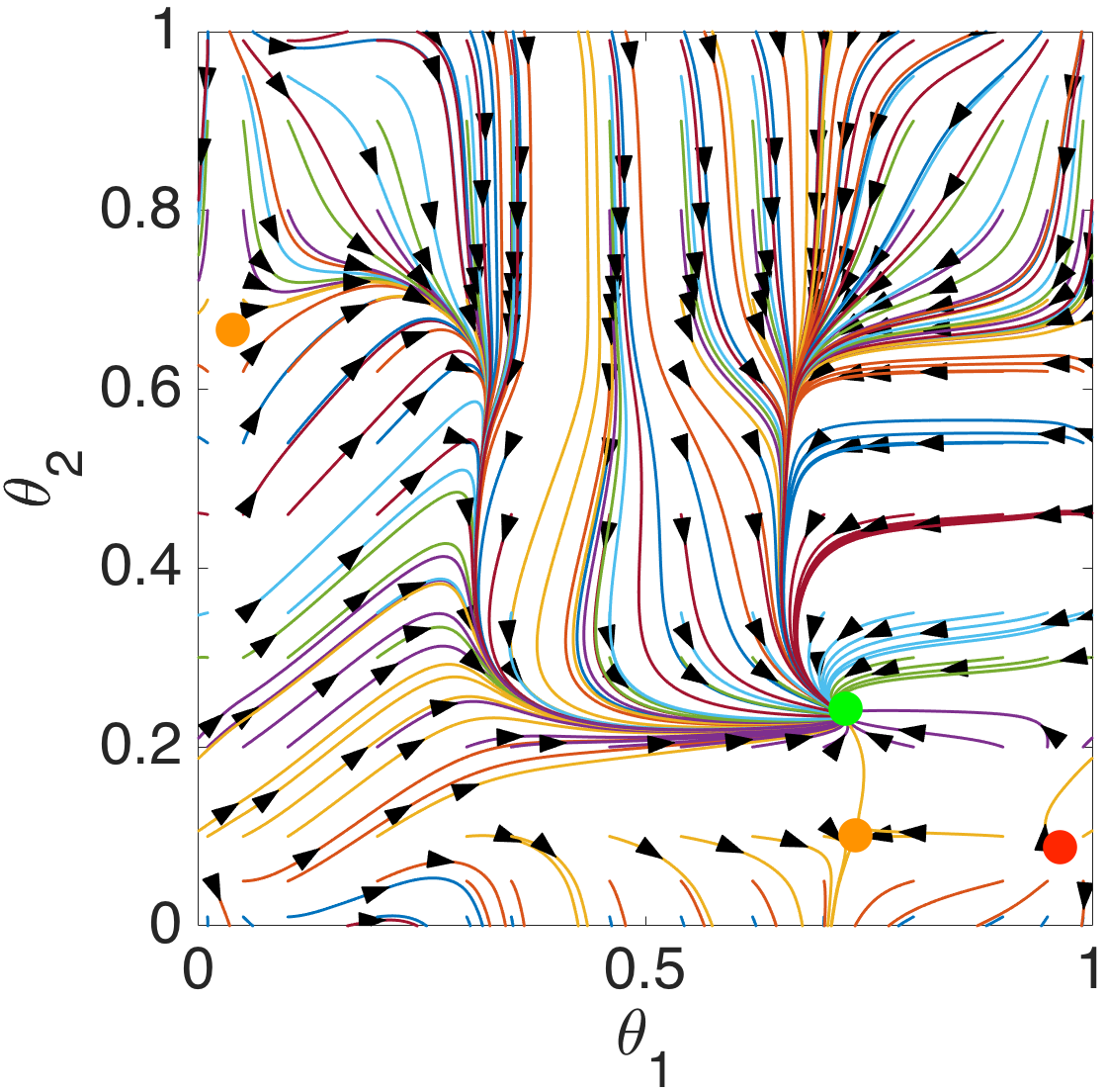
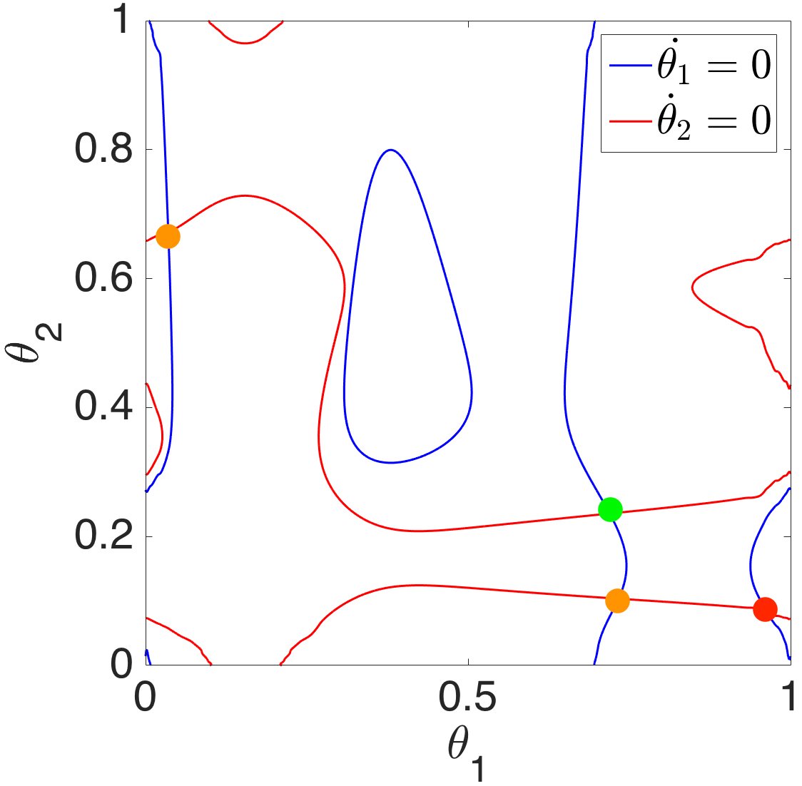
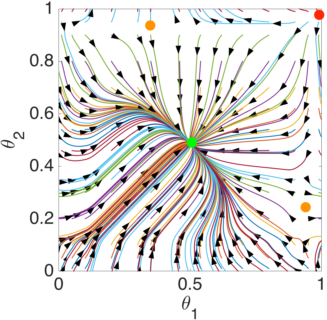
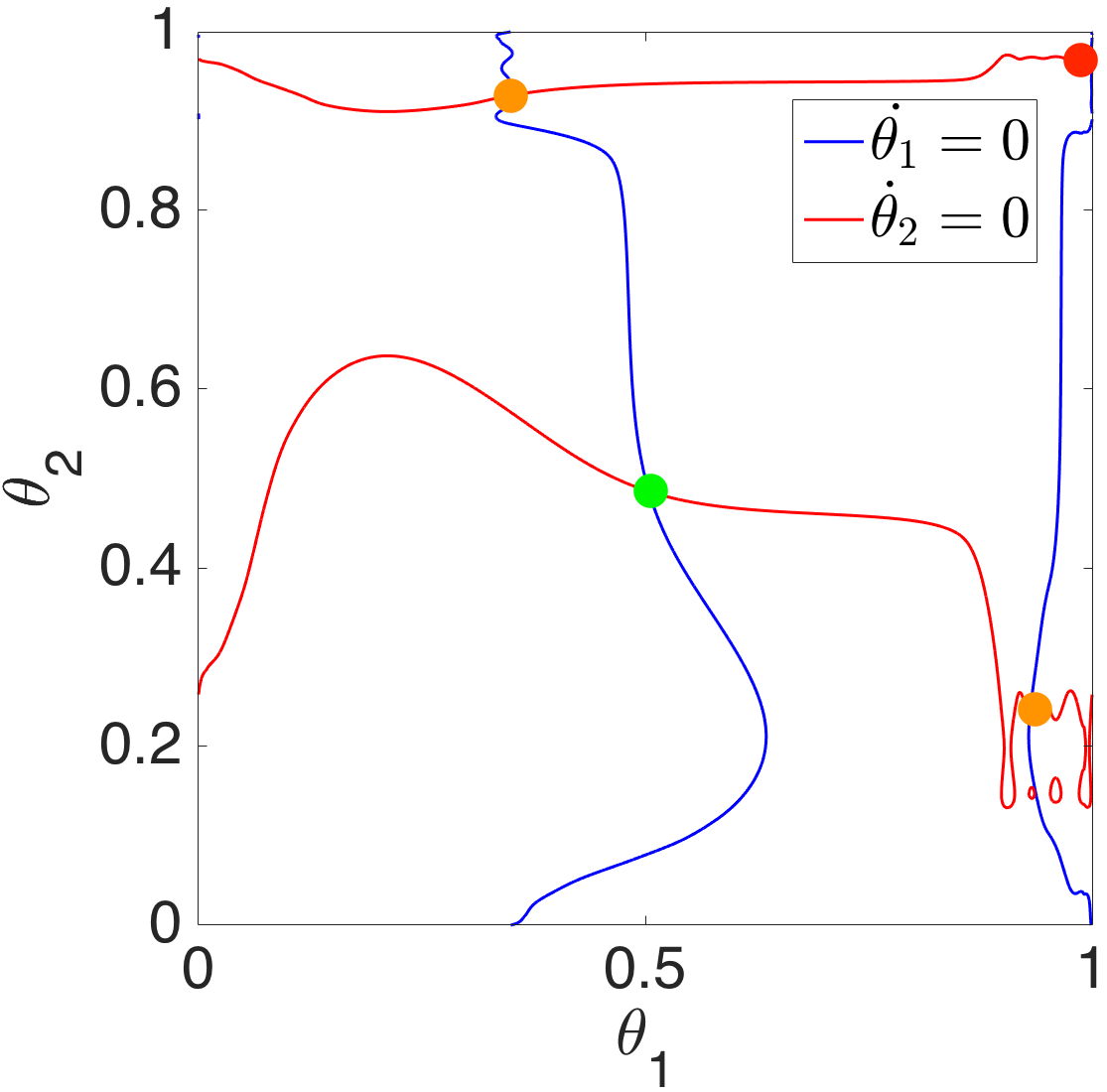
Figure 11: (Left to right) Phase planes and nullclines of Equations (25) when ${c}_{i}$’s satisfy Equation (26), $\delta I\approx 0.038$, and $I_{ext}=35.65$ (the nullclines of which are also shown in Figure 4 (right panel)), and $37.5$, respectively. Nullclines and fixed points are indicated as in Figure 4.

6 Equivalent perturbations

In this section, we will show that perturbing the intrinsic dynamics of each unit of the CPG can be equivalent to perturbing the coupling function $g$ or the coupling strengths ${c}_{i}$.

Recalling Equation (7), we show that, under an appropriate condition on the ${c}_{i}$’s, derived below, adding $I^{i}_{ext}$ to each neuron $i$ is equivalent to adding $dI_{j}$ to the coupling function $g(x_{i},x_{j})$ that connects neuron $i$ to its neighbor $j$, where $dI_{j}$ is the unique solution of

$$\left(\begin{array}[]{c}I_{ext}^{1}\\ \vdots\\ I_{ext}^{6}\end{array}\right)=\mathcal{C}\left(\begin{array}[]{c}dI_{1}\\ dI_{2}\\ dI_{3}\\ dI_{4}\\ dI_{5}\\ dI_{6}\end{array}\right):=\left(\begin{array}[]{cccccc}0&{c}_{5}&0&{c}_{1}&0&0\\ {c}_{4}&0&{c}_{7}&0&{c}_{2}&0\\ 0&{c}_{6}&0&0&0&{c}_{3}\\ {c}_{1}&0&0&0&{c}_{5}&0\\ 0&{c}_{2}&0&{c}_{4}&0&{c}_{7}\\ 0&0&{c}_{3}&0&{c}_{6}&0\end{array}\right)\left(\begin{array}[]{c}dI_{1}\\ dI_{2}\\ dI_{3}\\ dI_{4}\\ dI_{5}\\ dI_{6}\end{array}\right).$$ (33)

For example if the above equation has a unique solution, then since $I_{ext}^{1}={c}_{5}dI_{2}+{c}_{1}dI_{4}$, adding $I_{ext}^{1}$ to unit $1$ is equivalent to adding $dI_{2}$ to $g(x_{1},x_{2})$ and $dI_{4}$ to $g(x_{1},x_{4})$, i.e.,

$$\dot{x}_{1} = f(x_{1})+I_{ext}^{1}+{c}_{1}g(x_{1},x_{4})+{c}_{5}g(x_{1},x_{2})$$

$$= f(x_{1})+{c}_{5}dI_{2}+{c}_{1}dI_{4}+{c}_{1}g(x_{1},x_{4})+{c}_{5}g(x_{1},x_{2})$$

$$= f(x_{1})+{c}_{1}(g(x_{1},x_{4})+dI_{4})+{c}_{5}(g(x_{1},x_{2})+dI_{2}).$$

Equation (33) has a unique solution if the matrix $\mathcal{C}$ is non-singular, i.e., $\det\mathcal{C}\neq 0$. The matrix $\mathcal{C}$ can be written as

$$\mathcal{C}=\left(\begin{array}[]{cc}\mathcal{A}&\mathcal{B}\\ \mathcal{B}&\mathcal{A}\end{array}\right),$$

where $\mathcal{A}=\left(\begin{array}[]{ccc}0&{c}_{5}&0\\ {c}_{4}&0&{c}_{7}\\ 0&{c}_{6}&0\end{array}\right)$ and $\mathcal{B}=\mbox{diag}\,({c}_{1},{c}_{2},{c}_{3})$. Since

$$\left(\begin{array}[]{cc}I&0\\ I&I\end{array}\right)\left(\begin{array}[]{cc}\mathcal{A}&\mathcal{B}\\ \mathcal{B}&\mathcal{A}\end{array}\right)\left(\begin{array}[]{cc}I&0\\ -I&I\end{array}\right)=\left(\begin{array}[]{cc}\mathcal{A}-\mathcal{B}&\mathcal{B}\\ 0&\mathcal{A}+\mathcal{B}\end{array}\right),$$

where $I$ and $0$ are identity and zero matrices of appropriate sizes, and as shown in [13],

$$\det\left(\begin{array}[]{cc}\mathcal{A}-\mathcal{B}&\mathcal{B}\\ 0&\mathcal{A}+\mathcal{B}\end{array}\right)=\det(\mathcal{A}-\mathcal{B})\det(\mathcal{A}+\mathcal{B}),$$

we have

$$\det\mathcal{C}=\det(\mathcal{A}-\mathcal{B})\det(\mathcal{A}+\mathcal{B}) =\det\left(\begin{array}[]{ccc}-{c}_{1}&{c}_{5}&0\\ {c}_{4}&-{c}_{2}&{c}_{7}\\ 0&{c}_{6}&-{c}_{3}\end{array}\right)\det\left(\begin{array}[]{ccc}{c}_{1}&{c}_{5}&0\\ {c}_{4}&{c}_{2}&{c}_{7}\\ 0&{c}_{6}&{c}_{3}\end{array}\right)$$

$$=-({c}_{1}{c}_{2}{c}_{3}-{c}_{1}{c}_{6}{c}_{7}-{c}_{3}{c}_{4}{c}_{5})^{2}.$$

Hence, $\mathcal{C}$ is non-singular if and only if ${c}_{1}{c}_{2}{c}_{3}-{c}_{1}{c}_{6}{c}_{7}-{c}_{3}{c}_{4}{c}_{5}\neq 0.$

Next, we show that, perturbing each CPG unit by an external current can be equivalent to perturbing the coupling strengths. Recalling Equations (18) and Assumptions 2 and 4, adding $I^{i}_{ext}$ to each unit $i$ is equivalent to adding $\Delta_{i}:=\tilde{\omega}_{i}/H(2/3-{\eta};{\xi})$ to the contralateral coupling ${c}_{i}$, $i=1,2,3$, and keeping the other coupling strengths unchanged. Note that $\tilde{\omega}_{i}$ is of order $\epsilon$ and $H$ is of order 1, therefore $\Delta_{i}$ is of order $\epsilon$.

For example, adding $I_{ext}^{1}$ to unit $1$ is equivalent to adding $\tilde{\omega}_{1}$ to the corresponding phase equation, therefore by Assumption 4, we get

$$\dot{\phi}_{1} =\omega+\tilde{\omega}_{1}+{c}_{1}H(\phi_{4}-\phi_{1};{\xi})+{c}_{5}H(\phi_{2}-\phi_{1};{\xi})$$

$$=\omega+\tilde{\omega}_{1}+{c}_{1}H(2/3-{\eta};{\xi})+{c}_{5}H(\phi_{2}-\phi_{1};{\xi})$$

$$=\omega+\frac{\tilde{\omega}_{1}}{H(2/3-{\eta};{\xi})}H(2/3-{\eta};{\xi})+{c}_{1}H(2/3-{\eta};{\xi})+{c}_{5}H(\phi_{2}-\phi_{1};{\xi})$$

$$=\omega+\left(\frac{\tilde{\omega}_{1}}{H(2/3-{\eta};{\xi})}+{c}_{1}\right)H(2/3-{\eta};{\xi})+{c}_{5}H(\phi_{2}-\phi_{1};{\xi})$$

$$=\omega+(\Delta_{1}+{c}_{1})H(2/3-{\eta};{\xi})+{c}_{5}H(\phi_{2}-\phi_{1};{\xi}).$$

7 Discussion

In [1] we studied a homogeneous interconnected phase oscillator model for insect locomotion, and showed that the cyclic motion of each leg can be described by an oscillator, and that the insect’s speed increases with the common external input, $I_{ext}$, that each leg receives. At high speeds, when $I_{ext}$ is large, the model generates a unique stable tripod gait, as observed experimentally in cockroaches and fruit flies. However, for small $I_{ext}$, the model’s low speed dynamics include both stable forward and backward tetrapod gaits and a stable gait that has not been observed in insects, in which triple, double and single swing phases occur [1, Figure 29]. While fruit flies exhibit forward and backward tetrapod gaits at low speeds, the latter have only been seen in backward walking [16], and we therefore propose that brain or central nervous system inputs are likely used to switch among and select particular gaits.

In the present paper, we relax the assumption of homogeneous oscillators and allow heterogeneous ipsilateral external inputs denoted by $I_{ext}+{I_{ext}^{i}(t)}$ for $i=1,2,3$. We observe that, at low speed with small $I_{ext}$, and for appropriate choices of small heterogeneities ${I_{ext}^{i}(t)}$, $i=1,2,3$, the heterogeneous model generates only one stable approximate forward or backward tetrapod gait, as is expected experimentally. The selection of a stable gait is accomplished via sequences of saddle-node bifurcations in which all but one of the stable gaits disappears as particular currents ${I_{ext}^{i}(t)}$ increase. See Table 2 for a summary of the behaviors presented in Section 5.

At high speeds the single stable solution of the heterogeneous model is a tripod gait, as in the homogeneous case, and the model exhibits a transition from a forward or a backward tetrapod to a tripod gait as $I_{ext}$ increases (see Figure 11 for the former case).

In future work, we propose to allow the heterogeneous external inputs to be noisy and to study the resulting effects on the existence of gaits and their transitions.

References

- [1] Z. Aminzare, V. Srivastava, and P. Holmes. Gait transitions in a phase oscillator model of an insect central pattern generator. SIAM J. Appl. Dyn. Sys., 17(1):626–671, 2018.
- [2] R.M. Ghigliazza and P. Holmes. A minimal model of a central pattern generator and motoneurons for insect locomotion. SIAM J. Appl. Dyn. Sys., 3(4):671–700, 2004.
- [3] R.M. Ghigliazza and P. Holmes. Minimal models of bursting neurons: How multiple currents, conductances, and timescales affect bifurcation diagrams. SIAM J. Appl. Dyn. Sys., 3(4):636–670, 2004.
- [4] K.G. Pearson and J.F. Iles. Nervous mechanisms underlying intersegmental co-ordination of leg movements during walking in the cockroach. J. Exp. Biol., 58:725–744, 1973.
- [5] K.G. Pearson and J.F. Iles. Discharge patterns of coxal levator and depressor motoneurons of the cockroach, Periplaneta americana. J. Exp. Biol., 52:139–165, 1970.
- [6] K.G. Pearson. Central programming and reflex control of walking in the cockroach. J. Exp. Biol., 56:173–193, 1972.
- [7] E. Couzin-Fuchs, T. Kiemel, O. Gal, A. Ayali, and P. Holmes. Intersegmental coupling and recovery from perturbations in freely running cockroaches. J. Exp. Biol., 218(2):285–297, 2015.
- [8] R.P. Kukillaya, J.L. Proctor, and P. Holmes. Neuromechanical models for insect locomotion: Stability, maneuverability, and proprioceptive feedback. Chaos, 19(2):026107, 2009.
- [9] M.A. Schwemmer and T.J. Lewis. The theory of weakly coupled oscillators. In N.W. Schultheiss, A.A. Prinz, and R.J. Butera, editors, Phase Response Curves in Neuroscience: Theory, Experiment, and Analysis, pages 3–31. Springer New York, New York, NY, 2012.
- [10] Y. Kuramoto. Chemical Oscillations, Waves, and Turbulence, volume 19 of Springer Series in Synergetics. Springer-Verlag, Berlin, 1984.
- [11] C.R. Rao and S. Kumar Mitra. Generalized Inverse of Matrices and its Applications. John Wiley & Sons, Inc., New York-London-Sydney, 1971.
- [12] A. Yeldesbay, T. Tóth, and S. Daun. The role of phase shifts of sensory inputs in walking revealed by means of phase reduction. J. Comput. Neurosci., 44(3):313–339, 2018.
- [13] J.R. Silvester. Determinants of Block Matrices. Mathematical Gazette, 84(501):460–467, 2000.
- [14] R.P. Kukillaya and P. Holmes. A model for insect locomotion in the horizontal plane: Feedforward activation of fast muscles, stability, and robustness. J. Theor. Biol., 261 (2):210–226, 2009.
- [15] J. Proctor, R.P. Kukillaya, and P. Holmes. A phase-reduced neuro-mechanical model for insect locomotion: feed-forward stability and proprioceptive feedback. Phil. Trans. Roy. Soc. A, 368:5087–5104, 2010.
- [16] S.S. Bidaye, C. Machacek, Y. Wu, and B.J. Dickson. Neuronal control of drosophila walking direction. Science, 344:97–101, 2014.