Critical Dynamical Exponent of the Two-Dimensional Scalar $\phi^{4}$-Model with Local Moves

Abstract

We study the scalar one-component two-dimensional (2D) $\phi^{4}$-model by computer simulations, with local Metropolis moves. The equilibrium exponents of this model are well-established, e.g. for the 2D $\phi^{4}$-model $\gamma=1.75$ and $\nu=1$. The model has also been conjectured to belong to the Ising universality class. However, the value of the critical dynamical exponent $z_{c}$ is not settled. In this paper, we obtain $z_{c}$ for the 2D $\phi^{4}$-model using two independent methods: (a) by calculating the relative terminal exponential decay time $\tau$ for the correlation function $\langle\Phi(t)\Phi(0)\rangle$, and thereafter fitting the data as $\tau\sim L^{z_{c}}$, where $L$ is the system size, and (b) by measuring the anomalous diffusion exponent for the order parameter, viz., the mean-square displacement (MSD) $\langle\Delta\Phi^{2}(t)\rangle\sim t^{c}$ as $c=\gamma/(\nu z_{c})$, and from the numerically obtained value $c\approx 0.80$, we calculate $z_{c}$. For different values of the coupling constant $\lambda$, we report that $z_{c}=2.17\pm 0.03$ and $z_{c}=2.19\pm 0.03$ for the two methods respectively. Our results indicate that $z_{c}$ is independent of $\lambda$, and is likely identical to that for the 2D Ising model. Additionally, we demonstrate that the Generalized Langevin Equation (GLE) formulation with a memory kernel, identical to those applicable for the Ising model and polymeric systems, consistently captures the observed anomalous diffusion behaviour.

I Introduction

The $\phi^{4}$-model has become one of the most useful tools in studying of critical phenomena kleinert ; kaupuzes1 ; pelissetto ; amit . In two dimensions, the lattice version of the $\phi^{4}$-model is defined by the action ${\cal S}$ and Hamiltonian ${\cal H}$ as

$${\cal S}=\frac{{\cal H}}{k_{B}T}=-\beta\sum_{\langle ij\rangle}\phi_{i}\phi_{j}+\sum_{i}[\phi_{i}^{2}+\lambda(\phi_{i}^{2}-1)^{2}],$$ (1)

where $-\infty<\phi_{i}<\infty$ is the dynamical variable at site $i$, $\beta$ and $\lambda$ are two model constants. The summation of the first term in the r.h.s of Eq. (1) runs over all the nearest-neighbour spins, and for an $L\times L$ square lattice $0\leq(i,j)<L$. The order parameter for the $\phi^{4}$-model is defined as $\Phi=\sum_{i}\phi_{i}$, and the dynamics of the model is given by zinn ; lin

$$\dot{\phi_{i}} = -\Omega\frac{\partial{\cal S}}{\partial\phi_{i}}+\xi(i,t)$$ (2)

$$\langle\xi(i,t)\xi(i^{\prime},t^{\prime})\rangle = 2\Omega\delta(i-i^{\prime})\delta(t-t^{\prime}),$$ (3)

where $\xi(i,t)$ is a Gaussian noise term, and $\Omega$ represents the dissipation constant, which is related to the noise term by the Fluctuation-Dissipation relation (3).

The equilibrium properties of the model in relation to the critical phenomenon are well-studied. Earlier investigations of the two dimensional (2D) and three dimensional (3D) lattice $\phi^{4}$-model have indicated that the critical exponents $\gamma$ and $\nu$ are the same as these for the Ising model, e.g. in 2D, $\gamma=1.75$ and $\nu=1$ michev ; hasenbusch ; kaupuzes2 . Simultaneously, Monte Carlo simulations of the 2D lattice $\phi^{4}$-model have supported the idea that the $\phi^{4}$-model belongs to the Ising universality class mehling . Despite these advances in the equilibrium properties of the model, its critical dynamical properties are not settled.

As for the critical dynamical exponent, Blöte and Nightingale blote1 have analyzed three variations of Ising-type models with next-nearest-neighbour interactions, and found that they share the same critical exponents, not only $\gamma$ and $\nu$, but also the critical dynamical exponent $z_{c}$. Further works have supported their results both in 2D and 3D blote2 ; hasenbusch2 ; hohenberg . For the 2D Ising model $z_{c}$ has been determined quite precisely as $z_{c}=2.1665\pm 0.0012$ blote3 . For the critical dynamical exponent of the 2D $\phi^{4}$-model, $z\approx 2$ was mentioned in Ref. wolff , and the $\epsilon$-expansion method has shown that $z_{c}\in(2.04,2.14)$ nalimov . Further, $z_{c}$ has been measured using the heat bath algorithm, yielding $z_{c}=1.9\pm 0.21$ brower . In short, the value of the critical dynamical exponent for the $\phi^{4}$-model still remains to be determined with higher precision.

In this paper, we study the one-component 2D scalar $\phi^{4}$-model by computer simulations, i.e., Eq. (1), with local Metropolis moves. In order to settle the value of $z_{c}$, we employ two independent methods: (a) we calculate the relative terminal exponential decay time $\tau$ for the correlation function $\langle\Phi(t)\Phi(0)\rangle$, and thereafter fit the data as $\tau\sim L^{z_{c}}$, where $L$ is the system size, (b) we measure the mean-square displacement (MSD) of the order parameter $\langle\Delta\Phi^{2}(t)\rangle\sim t^{c}$ with $c=\gamma/(\nu z_{c})$, and from the numerically obtained value $c\approx 0.80$ we calculate $z_{c}$. We report that $z_{c}=2.17\pm 0.03$ and $z_{c}=2.19\pm 0.03$ for the two methods respectively. Our results suggest that $z_{c}$ is independent of $\lambda$, and is likely identical to that for the 2D Ising model.

Further, the numerical result $\langle\Delta\Phi^{2}(t)\rangle\sim t^{0.80}$ at the critical point means that $\Phi(t)$ undergoes anomalous diffusion. We argue that the physics of anomalous diffusion in the $\phi^{4}$-model at critical point is the same as for polymeric systems and the Ising model panja3 ; panja4 ; panja2a ; zhong , and therefore a GLE formulation that holds for the Ising model at criticality and for polymeric systems must also hold for the $\phi^{4}$-model. We obtain the force autocorrelation function for the $\phi^{4}$-model at $\dot{\Phi}=0$, and the results allow us to demonstrate the consistency between anomalous diffusion and its GLE formulation.

The paper is organised as follows. In Sec. II we introduce the $\phi^{4}$-model and the dynamics, and then show the results of the correlation term $\langle\Phi(t)\Phi(0)\rangle$ and the mean-square displacement of the order parameter; from both we measure the critical dynamical exponent. In Sec. III we briefly explain how the restoring force works, which naturally leads us to the Generalised Langevin Equation (GLE) formulation for the anomalous diffusion in the $\phi^{4}$-model, and verify the GLE formulation for anomalous diffusion. The paper is concluded in Sec. IV.

II The Measurement of the Critical Dynamical Exponent

II.1 The Model and the Dynamics

We consider the scalar one-component two-dimensional $\phi^{4}$-model on an $L\times L$ square lattice with periodic boundary conditions. The action is introduced in Eq. (1), and in this paper we focus on $\lambda\leq 1$.

We simulate the dynamics of the system, i.e. Eq. (2), using Monte Carlo moves, with the Metropolis algorithm: we randomly select a site $i$, for which we try to change the existing value $\phi_{i}$ to a new value $\phi_{i}^{\prime}$, given by

$$\phi_{i}^{\prime}=\phi_{i}+\Delta\phi\left(r-\frac{1}{2}\right),$$ (4)

where $r$ is a random number uniformly distributed within [0,1), and following Refs. hasenbusch ; kaupuzes2 , we set $\Delta\phi=3$. The resulting change of the action $\Delta{\cal S}$ after every attempted change in $\phi_{i}$ is calculated. The move is accepted if $\Delta{\cal S}\leq 0$; if not, then the move is accepted with the usual Metropolis probability $e^{-\Delta{\cal S}}$. With $\Delta\phi=3$, the acceptance rates are between $40\%$ and $60\%$.

In this paper, all simulations have been performed on a $3.40$GHz desktop PC running Linux. We mainly focus on three different values of $\lambda$, i.e. $\lambda=0.1,0.5,1.0$. The corresponding critical coupling constant $\beta_{c}$, obtained in Refs. kaupuzes2 ; bosetti , are listed in table 1.

$\lambda$	Value of $\beta_{c}$
0.1	0.60647915(35)
0.5	0.686938(10)
1.0	0.680601(11)

Table 1: The value of $\beta_{c}$ for $\lambda=0.1,0.5$ and $1.0$ kaupuzes2 ; bosetti .

Next, we use two independent methods to measure the dynamical exponent $z_{c}$.

II.2 Measurement of the Correlation function $\langle\Phi(t)\Phi(0)\rangle$

In the first method, we measure the correlation function $\langle\Phi(t)\Phi(0)\rangle$ of the order parameter. To obtain the corresponding data, we run our simulations for $5\times 10^{7}$ Monte Carlo steps per lattice site to thermalise the system. Subsequently, we keep taking snapshots of the system at regular intervals over a total time of $5\times 10^{8}$ Monte Carlo steps per lattice site, and compute the order parameter $\Phi$ at every snapshot. From this data set we calculate $\langle\Phi(t)\Phi(0)\rangle$.

We use system sizes $L=30,40,...,90$ for each value of $\lambda$. The required CPU time is about $45$ minutes for $L=30$, reaching about $6$ hours for $L=90$.

At long times we expect $\langle\Phi(t)\Phi(0)\rangle$ to behave as $\langle\Phi(t)\Phi(0)\rangle/\langle\Phi(0)\Phi(0)\rangle\sim\exp(-t/\tau)$, and define $Q(t)=-\ln\,[\langle\Phi(t)\Phi(0)\rangle/\langle\Phi(0)\Phi(0)\rangle]$, leading us to expect

$$Q(t)\sim t/\tau.$$ (5)

We then calculate the relative value of terminal decay time $\tau$ by collapsing the $Q(t)$ data to a reference for every value of $\lambda$. More explicitly, for every value of $\lambda$ we choose the $Q(t)$ data for $L=30$ as reference, set its $\tau$-value to unity, and then collapse the rest of the $Q(t)$ for other values of $L$ to that reference, which yields us the relative value of $\tau$ for that value of $\lambda$. As an example, Fig. 1(a) demonstrates this procedure: with a properly chosen relative value of $\tau$, the $\langle\Phi(t)\Phi(0)\rangle$ data for different system sizes collapse to the data of $L=30$.

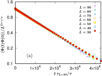
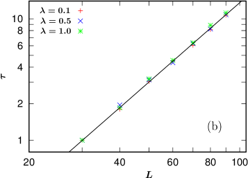
Figure 1: (color online) Measurement of $z_{c}$ from the $Q(t)$ data for different values of $\lambda$ at the critical point. (a) An example of the measurement process to obtain the relative value of terminal decay time $\tau$. In this figure $\lambda=0.1$ and $\tau_{L=30}$ is the terminal decay time of reference system size $L=30$. The data collapse (to the reference) is obtained by adjusting the relative values of terminal decay time for other system sizes; (b) Measurement of $z_{c}$ by fitting the data of the relative value of decay time $\tau$ as $\tau\sim L^{z_{c}}$.The symbols represent the simulation results of $\tau$ and the solid line corresponds to $\tau\sim L^{2.17}$.

At the critical temperature $\tau\sim\xi^{z_{c}}$, where $\xi$ is the correlation length. According to finite-size scaling theory, for finite system sizes $\xi$ needs to be replaced by $L$, i.e.,

$$\tau\sim L^{z_{c}}.$$ (6)

$\lambda$	$z_{c}$
$0.1$	2.17 $\pm$ 0.03
$0.5$	2.15 $\pm$ 0.03
$1.0$	2.20 $\pm$ 0.03

Table 2: The measured values of $z_{c}$ for the 2D $\phi^{4}$-model at different $\lambda$. The critical dynamical exponent $z_{c}$ is calculated by fitting the data of the relative value of $\tau$ as $\tau\sim L^{z_{c}}$. The results indicate that the value of $z_{c}$ is likely independent of $\lambda$, which allows us to produce a single estimate of $z_{c}$, viz., $z_{c}=2.17\pm 0.03$ (see main text).

The critical dynamical exponent $z_{c}$ is calculated by fitting the data of the relative value of $\tau$ with Eq. (6). Results of this procedure are shown in Fig. 1(b). The corresponding values of $z_{c}$ can be found in Table. 2. The error bars in Table 2 are obtained from the best fits of Fig. 1(b). These results indicate that the value of $z_{c}$ is likely independent of $\lambda$. If we do assume that, then we can combine the different numerical values for different $\lambda$ to produce a single estimate of $z_{c}$, viz., $z_{c}=2.17\pm 0.03$.

II.3 Mean-Square Displacement of the Order Parameter

In the second method, we focus on the measurement of the mean-square displacement of the order parameter at time $t$, given by

$$\langle\Delta\Phi^{2}(t)\rangle=\langle[\Phi(t)-\Phi(0)]^{2}\rangle.$$ (7)

To obtain the data of the MSD of the order parameter, we first thermalise the system with $2\times 10^{8}$ Monte Carlo moves per lattice site, then measure $\langle\Delta\Phi^{2}(t)\rangle$ in a further simulation over $2\times 10^{9}$ Monte Carlo moves per lattice site, using the shifting time window method.

For each value of $\lambda$, three different system sizes are used: $L=40,80,160$. For $L=40$, the simulation runs for about $5$ hours, and it takes about 3 days to obtain the results for $L=160$.

At short times ($t\approx 1$), the individual changes of $\Phi$ are uncorrelated; i.e., the mean-square displacement (MSD) of the order parameter must behave as $\langle\Delta\Phi^{2}(t)\rangle\sim L^{d}t$, where $d=2$ is the spatial dimension of the system.

At long times, $t\gtrsim L^{z_{c}}$, we expect $\langle\Phi(t)\Phi(0)\rangle=0$, which means that

$$\langle\Delta\Phi^{2}(t)\rangle\mathrel{\mathop{\approx}\limits_{t\gg L^{z_{c}}}}2\langle\Phi(t)^{2}\rangle\sim L^{d+\gamma/\nu},$$ (8)

which is an equilibrium quantity.

If we assume that the MSD is given by a simple power-law in the intermediate time regime ($1\lesssim t\lesssim L^{z_{c}}$), then we have

$$\langle\Delta\Phi^{2}(t)\rangle\sim t^{c},$$ (9)

where $c=\gamma/(\nu z_{c})$. Note that exactly the same behavior has been found in the Ising model walter ; zhong .

In order to measure the value of the exponent $c$ from $\langle\Delta\Phi^{2}(t)\rangle$, we need to focus on the intermediate time regime, i.e. we consider the MSD data in $(t_{min},t_{max})$ to estimate the exponent. From these data we calculate the exponent $c$ as numerical derivative as $\displaystyle c=\frac{1}{t_{max}-t_{min}}\sum\limits_{t=t_{min}}^{t_{max}-1}\frac{\ln\,\langle\Delta\Phi^{2}(t+1)\rangle-\ln\,\langle\Delta\Phi^{2}(t)\rangle}{\ln\,(t+1)-\ln\,t}$. In order to estimate $z_{c}$ for different $\lambda$ from these data, we use the data from the largest system size so that we can limit the influence of finite-size effects. From the numerically obtained $c$ we calculate $z_{c}$ and $c=\gamma/(\nu z_{c})$, which we present in Table. 3. These results, too, indicate that the value of $z_{c}$ is likely independent of $\lambda$. If we do assume that, then we can combine the different numerical values for different $\lambda$ to produce a single estimate of $z_{c}$, viz., $z_{c}=2.19\pm 0.03$.

$\lambda$	$z_{c}$
$0.1$	2.20$\pm$0.03
$0.5$	2.18$\pm$0.02
$1.0$	2.20$\pm$ 0.04

Table 3: The critical dynamical exponent $z_{c}$, which is obtained from the numerically obtained $c$ with $c=\gamma/(\nu z_{c})$, for the 2D $\phi^{4}$-model at different $\lambda$. The results, too, indicate that the value of $z_{c}$ is likely independent of $\lambda$, which allows us to produce a single estimate of $z_{c}$, viz., $z_{c}=2.19\pm 0.03$ (see main text).

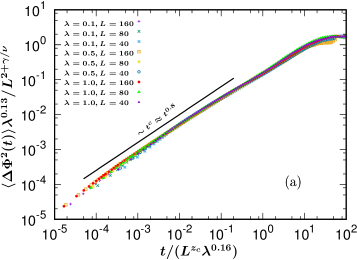
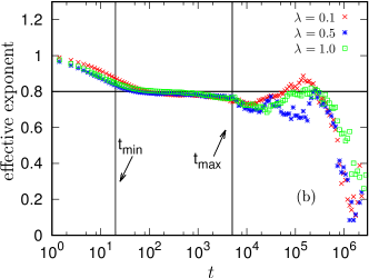
Figure 2: (color online) (a) The mean-square displacement (MSD) of the order parameter $\langle\Delta\Phi^{2}(t)\rangle$ in the $\phi^{4}$-model at the critical point. The MSD scales as $\langle\Delta\Phi^{2}(t)\rangle\sim L^{2}t^{c}$ where $c=\gamma/(\nu z_{c})$. The $x$ and $y$ axes are scaled with $\lambda$-dependent numerical scale factors to achieve good quality data collapse for different $\lambda$. The solid line denotes the power-law behavior shown in Eq. (8). (b) The effective exponents, i.e., the numerically differentiated $d\,\ln(\langle\Delta\Phi^{2}(t)\rangle)/d\,\ln(t)$, of the MSD of the order parameter for different $\lambda$. The system sizes are $L=160$ and the time period for calculating the exponent $c$ is $t\in(t_{min},t_{max})$, where $t_{min}\sim 1$ and $t_{max}\sim L^{z_{c}}$.

The corresponding data for the MSD of $\Phi(t)$ for $80\leq L\leq 160$ for different values of $\lambda$ are shown in Fig. 2. The small deviation in Fig. 2 at late times is caused by periodic boundary conditions: they are different when free boundary conditions are utilised. (Exactly the same effect has been observed in our earlier work on the Ising model zhong . Verification of the boundary effects is therefore not shown here, since the deviations from the power-law do not scale with $L$, and consequently are not relevant in the scaling limit.)

In conclusion, the critical dynamical exponent $z_{c}$ obtained with two independent methods demonstrate that $z_{c}=2.17\pm 0.03$ or $z_{c}=2.19\pm 0.03$ for different values of $\lambda$ in the 2D scalar $\phi^{4}$-model. Both results are consistent to the value of $z_{c}$ for the 2D Ising model ($2.1665\pm 0.0012$). In other words, our results indicate that $z_{c}$ is independent of $\lambda$, and is likely identical to that for the 2D Ising model.

III The GLE formulation of the anomalous diffusion in the $\phi^{4}$-model

In Sec. II.3 we numerically obtained that, in the intermediate time regime, the MSD of the order parameter in the $\phi^{4}$-model behaves as

$$\langle\Delta\Phi^{2}(t)\rangle\sim L^{2}t^{0.80}.$$ (10)

This means that, at the critical point, the order parameter exhibits anomalous diffusion. The same behavior has been observed in the Ising model walter . The physics of anomalous diffusion in the Ising model has been thoroughly analysed in Ref. zhong , where it has also been demonstrated that the physics is identical to that for polymeric systems panja2a ; panja3 ; panja4 ; panja1 ; panja3b ; panja3c ; panja3d ; panja2 .

Both in the Ising model and polymeric systems, the anomalous diffusion stems from time-dependent restoring forces which lead to the GLE formulation. Translated to the $\phi^{4}$-model, the physics of the restoring force can be described as follows.

Imagine that the order parameter locally changes by an amount $\delta\phi$ due to thermal fluctuations at $t=0$. Due to the interactions among the spins dictated by the Hamiltonian, the system will react to the change in $\delta\phi$. This reaction will be manifest in the two following ways: $(a)$ the system will to some extent adjust to the change of $\delta\phi$, however it will take some time, and $(b)$ during this time the order parameter will also readjust to the persisting value of $\Phi$, undoing at least part of $\delta\phi$. It is the latter that we interpret as the result of inertia that resists change in $\Phi$, and the resistance itself acts as the restoring force to the changes in the order parameter.

III.1 The GLE formulation for the anomalous diffusion in the $\phi^{4}$-model

In the Ising model and polymeric systems, the restoring force has led to the GLE description for the anomalous diffusion zhong ; panja3 ; panja4 . We now import that for the $\phi^{4}$-model, with a time-dependent memory function $\mu(t)$ arising out of the restoring forces. The GLE formulation for the anomalous diffusion is described as

$$\zeta\dot{\Phi}(t)=f(t)+q_{1}(t)$$ (11a)

$$f(t)=-\int_{0}^{t}dt^{\prime}\mu(t-t^{\prime})\,\dot{\Phi}(t^{\prime})+q_{2}(t).$$ (11b)

Here $f(t)$ is the internal force, $\zeta$ is the “viscous drag” on $\Phi(t)$, $\mu(t-t^{\prime})$ is the memory kernel, $q_{1}(t)$ and $q_{2}(t)$ are two noise terms satisfying $\langle q_{1}(t)\rangle=\langle q_{2}(t)\rangle=0$, and the fluctuation-dissipation theorems (FDTs) $\langle q_{1}(t)\,q_{1}(t^{\prime})\rangle\propto\zeta\delta(t-t^{\prime})$ and $\langle q_{2}(t)\,q_{2}(t^{\prime})\rangle\propto\mu(t-t^{\prime})$ respectively.

Equation (11b) can be inverted to write as

$$\dot{\Phi}(t)=-\int_{0}^{t}dt^{\prime}\,a(t-t^{\prime})f(t^{\prime})+\omega(t).$$ (12)

The noise term $\omega(t)$ similarly satisfies $\langle\omega(t)\rangle=0$, and the FDT $\langle\omega(t)\omega(t^{\prime})\rangle=a(|t-t^{\prime}|)$. Then $a(t)$ and $\mu(t)$ are related to each other in the Laplace space as $\tilde{a}(s)\tilde{\mu}(s)=1$.

To combine Eq. (11a) and (11b), we obtain

$$\zeta\dot{\Phi}(t)=-\int_{0}^{t}dt^{\prime}\mu(t-t^{\prime})\,\dot{\Phi}(t^{\prime})+q_{1}(t)+q_{2}(t).$$ (13)

or

$$\dot{\Phi}(t)=-\int_{0}^{t}dt^{\prime}\theta(t-t^{\prime})\,[q_{1}(t)+q_{2}(t)].$$ (14)

where in the Laplace space $\tilde{\theta}(s)[\zeta+\tilde{\mu}(s)]=1$. With $t>t^{\prime}$, without any loss of generality, using Eq. (14) the result of the velocity autocorrelation is

$$\langle\dot{\Phi}(t)\dot{\Phi}(0)\rangle\sim\theta(t-t^{\prime}),$$ (15)

where $\theta(t)$ can be calculated by Laplace inverting the relation $\tilde{\theta}(s)[\zeta+\tilde{\mu}(s)]=1$.

If $\mu(t)$ behaves as a power-law in time with an exponential cutoff such as

$$\mu(t)\sim L^{-2}t^{-c}\exp(-t/\tau),$$ (16)

then we have panja4

$$\langle\dot{\Phi}(t)\dot{\Phi}(t^{\prime})\rangle=-\theta(t-t^{\prime})\sim-L^{2}(t-t^{\prime})^{c-2}\qquad\text{for}\quad t\leq\tau.$$ (17)

By integrating Eq. (17) twice in time (the Green-Kubo relation), we obtain

$$\langle\Delta\Phi^{2}(t)\rangle\sim L^{2}t^{c}\qquad\text{for}\quad t\leq\tau.$$ (18)

The form $\mu(t)\sim L^{-2}t^{-c}$ not only obtains the anomalous exponent for the mean-square displacement, but also the correct $L$-dependent prefactor to achieve the data collapse in Fig. 2, i.e., if $\mu(t)\sim L^{-2}t^{-c}$, then $\langle\Delta\Phi^{2}(t)\rangle\sim L^{2}t^{c}$.

III.2 Verification of the first equation of the GLE and the power-law behaviour of $\mu(t)$

We now numerically verify our proposed GLE formulation, including the form of $\mu(t)$ as stated in Eq. (15) for anomalous diffusion in the $\phi^{4}$-model.

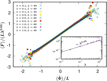
Figure 3: (color online) The linear relation Eq. (11a) between the average internal force $\langle f\rangle$ and $\langle\dot{\Phi}\rangle$ for different $\lambda$. Numerically, we find (inset) that the viscous drag $\zeta$ behaves as $\zeta\sim\lambda^{0.65}$.

First, in order to verify Eq. (11a), note that in the $\phi^{4}$-model, the force within the system can be directly calculated as

$$f=-\frac{1}{L^{2}}\sum_{i=0}^{N}\frac{\partial{\cal S}}{\partial\phi_{i}}\frac{\partial\phi_{i}}{\partial\Phi}=-\frac{1}{L^{2}}\sum_{i=0}^{N}\frac{\partial{\cal S}}{\partial\phi_{i}}.$$ (19)

By taking ensemble averages on both sides of Eq. (11a) we obtain

$$\langle f(t)\rangle=\zeta\langle\dot{\Phi}\rangle.$$ (20)

This linear relation is demonstrated in Fig. 3. Additionally, in the inset we plot the viscous drag $\zeta$ as a function of $\lambda$, and numerically obtain $\zeta\sim\lambda^{0.65}$.

Next we verify the power-law behaviour of $\mu(t)$ (Eq. (15)) following the FDT $\langle f(t)f(t^{\prime})\rangle|_{\dot{\Phi}=0}=\mu(t-t^{\prime})$.

We start with a thermalised system at $t=0$. For $t>0$ we fix the value of $\Phi$ (without freezing the whole system), which we achieve by performing non-local spin-exchange moves, i.e., at each move, we choose two lattice site $i$ and $j$ at random, and attempt to change the spin values to $\phi_{i}^{\prime}=\phi_{i}+\Delta\phi$ and $\phi_{j}^{\prime}=\phi_{j}-\Delta\phi$. We calculate the change in the energy $\Delta{\cal S}$ before and after every attempted move, and accept or reject the move with the Metropolis acceptance probability. While performing spin-exchange dynamics, we keep taking snapshots of the system at regular intervals, and compute, at every snapshot (denoted by $t$), the force $f(t)$ from Eq. (19).

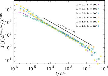
Figure 4: (color online) Behaviour $\Gamma(f)\sim t^{-0.8}$ for different $\lambda$ in the intermediate time regime following Eq. (22), then following the FDT, we have $\mu(t)\sim t^{-0.8}$. The extra $\lambda$-dependent factor $\lambda^{0.35}$ is introduced numerically to collapse the data for different $\lambda$ at intermediate times. Further, $z_{c}=2.17$ has been used here to collapse the data.

We notice that since simulations are performed for finite systems with $\Phi$ fixed at its $t=0$ value, we will in any particular run have a non-zero value of $\langle f(t)\rangle$ acting to sustain the initial value of $\Phi$ zhong . Thus we calculate the quantity

$$\Gamma(f)=\langle f(t)f(t^{\prime})\rangle-\langle f(t)\rangle\langle f(t^{\prime})\rangle,$$ (21)

which we expect to represent $\mu(t-t^{\prime})$ for all values of $\lambda$, i.e.,

$$\Gamma(f)\sim L^{-2}t^{-c}\approx L^{-2}t^{-0.80}.$$ (22)

The relation (22) is verified in Fig. 4.

IV Conclusion

In this paper, we have measured the critical dynamical exponent $z_{c}$ in the $\phi^{4}$-model using two independent methods: (a) by calculating the relative terminal exponential decay time $\tau$ for the correlation function $\langle\Phi(t)\Phi(0)\rangle$, and thereafter fitting the data as $\tau\sim L^{z_{c}}$, and (b) by measuring the mean-square displacement (MSD) of the order parameter $\langle\Delta\Phi^{2}(t)\rangle\sim t^{c}$ with $c=\gamma/(\nu z_{c})$, and $z_{c}$ is calculated from the numerically obtained value $c\approx 0.80$. For different values of the coupling constant $\lambda$, we report that $z_{c}=2.17\pm 0.03$ and $z_{c}=2.19\pm 0.03$ for these two methods respectively. Our results indicate that $z_{c}$ is independent of $\lambda$, and is likely identical to that for the 2D Ising model.

Further, the numerical result $\langle\Delta\Phi^{2}(t)\rangle\sim t^{0.80}$ at the critical point means that $\Phi(t)$ undergoes anomalous diffusion. We have argued that the physics of anomalous diffusion in the $\phi^{4}$-model at the critical point is the same as for polymeric systems and the Ising model panja3 ; panja4 ; zhong , and therefore a GLE formulation that holds for the Ising model at criticality and for polymeric systems must also hold for the $\phi^{4}$-model. We obtain the force autocorrelation function for the $\phi^{4}$-model at $\dot{\Phi}=0$, and the results allow us to demonstrate the consistency between anomalous diffusion and its GLE formulation. In comparison to the Ising model, since $\Phi$ is a continuous order parameter and there is a proper definition of the internal force, we believe that the $\phi^{4}$-model is a better choice to verify the FDT for the GLE formulation.

Finally, we note that we have confined ourselves to the range $\lambda\in(0,1]$. It is clearly possible to extend our study to larger values of $\lambda$, in particular to $\lambda\rightarrow\infty$, where the model converges to the Ising model, but not without facing additional challenges, as follows. The thermal fluctuations decrease with increasing $\lambda$, and the effective interactions among the fields become weaker kaupuzes2 . For large $\lambda$, the self-energy term of the fields in the Hamiltonian becomes large. The step size has to be chosen small, otherwise it will lead to many rejected moves. As a consequence, the system gets trapped within narrow bands on the energy landscape. Our preliminary attempts to simulate the model at large $\lambda$ reveal that these traps give rise to artifacts (e.g., in force autocorrelation function at fixed $\Phi$) that are not easy to get rid of. These are issues we will explore in the future.

Acknowlegement

W.Z. acknowledges financial support from the China Scholarship Council (CSC).

References

- (1) H. Kleinert, V. Schulte-Frohlinde, Critical Properties of Theories, World Scientific, Singapore (2001).
- (2) J. Kaupužs, Int. J. Mod. Phys. A 27 1250114 (2012).
- (3) A. Pelissetto, E.Vicari, Phys. Rep. 368, 549 (2002).
- (4) D. J. Amit, Field Theory, the Renormalization Group, and Critical Phenomena, World Scientific, Singapore (1984).
- (5) J. Zinn-Justin, Quantum Field Theory and Critical Phenomena, Clarendon Press, New York (1996).
- (6) Y. Lin and F. Wang, Phys. Rev. E 93, 022113 (2016).
- (7) A. Michev, D. W. Heermann, and K. Binder, J. Stat. Phys. 44, 749 (1986).
- (8) M. Hasenbusch, J. Phys. A 32, 4851 (1999).
- (9) J. Kaupužs, R. V. N. Melnik and J. Rimšāns, Int. J. Mod. Phys. C 27, 1650108 (2016).
- (10) B. Mehling, B. M. Forrest, Z. Phys. B 89, 89 (1992).
- (11) H. W. J. Blöte, M. P. Nightingale, Physica A 251, 211 (1998).
- (12) H. W. J. Blöte, E. Luijten, and J. R. Heringa, J. Phys. A 28, 6289 (1995).
- (13) M. Hasenbusch, K. Pinn, and S. Vinti, Phys. Rev. B 59, 11471 (1999).
- (14) P. C. Hohenberg and B. I. Halperin, Rev. Mod. Phys. 49, 435 (1977).
- (15) M. P. Nightingale and H. W. J. Blöte, Phys. Rev. Lett. 76, 4548(1996).
- (16) K. H. Hoffmann, M. Schreiber (eds), Computational Physics, Springer, Berlin,(1996).
- (17) M. Y. Nalimov, V. A. Sergeev, and L. Sladkoff, Theor. Math. Phys. 159, 499 (2009).
- (18) R. C. Brower, P. Tamayo, Phys. Rev. Lett. 62, 1087 (1989).
- (19) J. -C. Walter, G. T. Barkema, Physica A, 418, 78(2015).
- (20) D. Panja, J. Stat. Mech. (JSTAT) L02001 (2010).
- (21) D. Panja, J. Stat. Mech. (JSTAT) P06011 (2010).
- (22) D. Panja, J. Phys.: Condens. Matter 23, 105103 (2011).
- (23) W. Zhong, D. Panja, G. T. Barkema, and R. C. Ball, Phys. Rev. E 98, 012124(2018).
- (24) P. Bosetti, B. De Palma, and M. Guagnelli, Phys. Rev. D 92, 034509 (2015).
- (25) D. Panja, G. T. Barkema and R. C. Ball, J. Phys.: Condens. Matter 19, 432202 (2007).
- (26) D. Panja, G. T. Barkema and R. C. Ball, J. Phys.: Condens. Matter 20, 075101 (2008).
- (27) D. Panja and G. T. Barkema, Biophys. J. 94, 1630 (2008).
- (28) H. Vocks, D. Panja, G. T. Barkema and R. C. Ball, J. Phys.: Condens. Matter 20, 095224 (2008).
- (29) D. Panja and G. T. Barkema, J. Chem. Phys. 131, 154903 (2009).