Thermal convection in rotating spherical shells: temperature-dependent internal
heat generation using the example of triple-$\alpha$ burning in neutron stars

Abstract

We present an extensive study of Boussinesq thermal convection including a temperature-dependent internal heating source, based on numerical three-dimensional simulations. The temperature dependence mimics triple-$\alpha$ nuclear reactions and the fluid geometry is a rotating spherical shell. These are key ingredients for the study of convective accreting neutron star oceans. A dimensionless parameter ${\rm Ra}_{n}$, measuring the relevance of nuclear heating, is defined. We explore how flow characteristics change with increasing ${\rm Ra}_{n}$ and give an astrophysical motivation. The onset of convection is investigated with respect to this parameter and periodic, quasiperiodic, chaotic flows with coherent structures, and fully turbulent flows are exhibited as ${\rm Ra}_{n}$ is varied. Several regime transitions are identified and compared with previous results on differentially heated convection. Finally, we explore (tentatively) the potential applicability of our results to the evolution of thermonuclear bursts in accreting neutron star oceans.

I Introduction

Convection is responsible for transporting angular momentum and for the generation of magnetic fields in cosmic bodies - in particular in the Earth’s outer core Dormy and Soward (2007). Surface zonal patterns observed on the gas giants (Jupiter and Saturn) Christensen (2002); Heimpel and Aurnou (2007) and the ice giants (Uranus and Neptune) Aurnou et al. (2007) are thought to be maintained by convection within deeper layers. In the case of stars, the differential rotation and meridional circulation observed in the Sun Miesch et al. (2006) and in main sequence stars Matt et al. (2011) are modelled using compressible convective models. The latter also seems to be quite sufficient to explain the magnetic fields of isolated white dwarfs Isern et al. (2017).

Convection, driven by nuclear burning, is also believed to be important in accreting white dwarfs and neutron stars. For the former, fully three-dimensional simulations in Jacobs et al. (2016) of the convective dynamics establish the conditions for runaways (thermonuclear explosions) in sub-Chandrasekhar-mass white dwarfs. Neutron stars that accrete matter from a companion star build up a low-density fluid layer of predominantly light elements (hydrogen and helium) on top of the star’s solid crust, forming a surface ocean (see Chamel and Haensel (2008) for a discussion of the conditions for solidification at the ocean-crust interface). Thermonuclear burning of these elements as they settle in the ocean can be unstable, giving rise to the phenomenon of Type I X-ray bursts (X-ray bursts are a sudden increase in the X-ray luminosity of a source as radiation from the runaway thermonuclear reactions escapes, see Strohmayer and Bildsten (2006) for a general review, and should not be confused with the convective bursts studied in the planetary literature Chossat (2000); Heimpel and Aurnou (2012).) The energy produced in the thermonuclear runaways cannot be dissipated by radiative transfer, and then convection sets in. In the case of neutron stars, surface patterns known as burst oscillations (for a review see Watts (2012)) are observed to develop frequently during these thermonuclear explosions, motivating an interest in convective patterns Watts (2012); Malone et al. (2014); Keek and Heger (2017a). Burst oscillations appear as modulation of the X-ray luminosity in the aftermath of a Type I X-ray burst. Possible explanations of this phenomenon involve flame spreading Spitkovsky et al. (2002); Cavecchi et al. (2013, 2015, 2016); Mahmoodifar and Strohmayer (2016) or global modes of oscillation of the ocean Heyl (2004); Piro and Bildsten (2005) (see also Chambers et al. (2018) in the case of superbursts) but we are still far from having a complete understanding.

For the above-mentioned reasons many numerical, analytic and experimental studies are devoted to this field. Good reviews can be found in the literature, see for instance Jones (2007) on convection in the Earth’s outer core, Jones (2011) on planetary dynamos or Olson (2011) which focuses on experiments in rotating spherical geometry. In the case of convective stellar interiors the review Gilman (2000) gives a fluid dynamics perspective, focusing on the effect of rotation in solar convection. Finally, the recent review of Arnett and Meakin (2016) describes the state of the art of stellar simulations, covering a wide range of astrophysical applications.

Current astrophysical hydrodynamical numerical codes, incorporating nuclear burning physics, are set up in square geometries Malone et al. (2011, 2014); Zingale et al. (2015); Cavecchi et al. (2013, 2015, 2016) and are thus local in nature. For this reason the study of patterns of convection in a rotating spherical geometry (global patterns) generated by nuclear burning, as proposed in this paper, is novel and of importance. The study is restricted to Boussinesq convection and does not incorporate compositional gradients, which may be a substantial simplification in the astrophysical context. However, this approximation makes sense when the focus is to study basic hydrodynamical mechanisms in tridimensional domains, as is commonly adopted in the context of planetary atmospheres (see for instance  Heimpel and Aurnou (2007)). This knowledge will provide a starting point for further global studies incorporating more complex physics, opening the way for a deeper understanding of stellar processes.

Boussinesq and anelastic thermal convection in rotating spherical shells with differential heating mechanisms have been studied in considerable detail over the past decades MacPherson (1977); Sumita and Olson (2002); Gibbons et al. (2007); Dietrich et al. (2016) (among many others), but in the context of planetary cores and dynamos. The secular cooling of planetary cores is modelled by internal buoyancy sources and the heat flux is assumed to be nonuniform in the lateral direction of the outer boundary, to mimic the thermal structure of the lower rocky mantle. The physical characteristics of accreting neutron stars are however quite different Watts (2012). The internal heat released in thermonuclear burning reactions is strongly dependent on temperature: helium flashes, which we consider in this paper, are caused by the extremely temperature-sensitive triple-alpha reaction Clayton (1984). In addition, the flow velocity boundary conditions are stress-free rather than zero. This is important for the generation of zonal patterns, as has been shown in studies of planetary atmospheres Aurnou and Olson (2001); Christensen (2002); Heimpel and Aurnou (2007).

Changing mechanical boundary conditions from nonslip to stress-free, or decreasing the gap width of the shell (more realistic for convection in atmospheres), results in a strong zonal wind generation and quasi-geostrophic flow, even at supercritical regimes Aurnou and Olson (2001). On the giant planets (Jupiter and Saturn) the strong equatorial zonal flow is positive (prograde, eastward) Christensen (2002); Heimpel and Aurnou (2007) while in ice giants (Uranus and Neptune) it is negative (retrograde, westward) Aurnou et al. (2007). This transition from prograde to retrograde zonal flow was interpreted in Aurnou et al. (2007) as a consequence of vigorous mixing leading to a progressive domination of inertial forces with respect to Coriolis forces. The prograde zonal flow was also found to be quite robust when considering the effect of density stratification Jones and Kuzanyan (2009).

The focus of this study is to investigate thermal convection driven by nuclear burning heat sources, as occurs in the envelopes of accreting neutron stars, by means of direct numerical simulations (DNS) in a rotating spherical shell geometry. The convective patterns and their mixing properties, arising prior to ignition, are important for the modelling of thermonuclear bursts Watts (2012). Convection tends to mix the fuel and ashes Woosley et al. (2004), altering nuclear reactions. We chose a very similar set-up to that used for planetary atmospheres Gastine et al. (2013), although with a different buoyancy driving mechanism, allowing a careful comparison. We find that the flows excited by heat released from nuclear reactions exhibit relevant features typical of planetary atmospheres.

The paper is organized as follows. In § II we introduce the formulation of the problem, and the numerical method used to obtain the solutions. In § III the type of solutions with increasing ${\rm Ra}_{n}$ are described and we analyse their physical properties, flow patterns, force balance and time scales. Section § IV contains a discussion of the application to accreting neutron star oceans, and finally § V summarises the results obtained.

II Model

We consider Boussinesq convection of a homogeneous fluid of density $\rho$, thermal diffusivity $\kappa$, thermal expansion coefficient $\alpha$, and dynamic viscosity $\mu$. The fluid fills the gap between two concentric spheres, rotating about an axis of symmetry with constant angular velocity ${\bf\Omega}=\Omega{\mathbf{k}}$, and it is subject to radial gravitational field ${\bf g}=-\gamma\mathbf{r}$ ($\gamma$ is constant and $\mathbf{r}$ the position vector). In the Boussinesq approximation $\kappa$, $\alpha$ and $\mu$ are considered constants, and the simple equation of state $\rho=\rho_{0}(1-\alpha(T-T_{0}))$ is assumed in just the gravitational term. In the other terms a reference state $(\rho_{0},T_{0})$ is assumed (see for instance Pedlosky (1979)).

Previous studies have mainly considered two different thermal driving mechanisms Chandrasekhar (1981); Dormy et al. (2004). Convection may be driven by an imposed temperature gradient on the boundaries and/or by a uniform distribution of heat sources $q$. In contrast to this, the present study considers a temperature-dependent heat souce $q$, and fixed temperature at the boundaries. Heat generation that depends on temperature (and also on density and nuclear species mass fraction) is used to model thermonuclear reactions in stellar interiors Clayton (1984).

In the following, we start by describing the widely-used system of equations without internal heat generation, and afterwards introduce the new system including a temperature-dependent heat source term.

II.1 The equations and the method

In the absence of internal heat sources, and considering perfectly conducting boundaries, $T(r_{i})=T_{i}$ and $T(r_{o})=T_{o}$ ($r_{i}$ and $r_{o}$ being the radius of the inner and outer boundary, respectively), the purely conductive state, in which the fluid is at rest, is given by ${\mathbf{v}}=0$ and $T_{c}(r)=T_{0}+\eta d\Delta T(1-\eta)^{-2}r^{-1}$, where ${\mathbf{v}}$ is the velocity field, $\eta=r_{i}/r_{o}$ the aspect ratio, $d=r_{o}-r_{i}$ the gap width, $\Delta T=T_{i}-T_{o}$ the temperature difference, and $T_{0}=T_{i}-\Delta T(1-\eta)^{-1}$, a reference temperature.

Following the same formulation as in Simitev and Busse (2003) the mass, momentum and energy equations are written in the rotating frame of reference and in terms of the velocity field ${\mathbf{v}}$ and the temperature perturbation from the conduction state $\Theta=T-T_{c}$. With units $d=r_{o}-r_{i}$ for the distance, $\nu^{2}/\gamma\alpha d^{4}$ for the temperature, and $d^{2}/\nu$ for the time, the equations are

$$\nabla\cdot{\mathbf{v}}=0,$$ (1)

$$\partial_{t}{\mathbf{v}}+{\mathbf{v}}\cdot\nabla{\mathbf{v}}+2{\rm Ta}^{1/2}\mathbf{k}\times{\mathbf{v}}=-\nabla p^{*}+\nabla^{2}{\mathbf{v}}+\Theta\mathbf{r},$$ (2)

$$\Pr\left(\partial_{t}\Theta+{\mathbf{v}}\cdot\nabla\Theta\right)=\nabla^{2}\Theta+{\rm Ra}\eta(1-\eta)^{-2}r^{-3}\mathbf{r}\cdot{\mathbf{v}},$$ (3)

where $p^{*}$ is the dimensionless pressure containing all the potential forces. The centrifugal force is neglected since $\Omega^{2}/\gamma\ll 1$ in stellar interiors. The system is governed by four non-dimensional parameters, the aspect ratio $\eta=r_{i}/r_{o}$ and the Rayleigh ${\rm Ra}$, Prandtl $\Pr$, and Taylor ${\rm Ta}$ numbers. These numbers are defined by

$${\rm Ra}=\frac{\gamma\alpha\Delta Td^{4}}{\kappa\nu},\quad{\rm Ta}^{1/2}=\frac{\Omega d^{2}}{\nu},\quad\Pr=\frac{\nu}{\kappa}.$$ (4)

If in addition to the externally imposed temperature gradient we are also interested in considering internal heat sources the energy equation (3) becomes

$$\Pr\left(\partial_{t}\Theta+{\mathbf{v}}\cdot\nabla\Theta\right) =\nabla^{2}\Theta+{\rm Ra}\eta(1-\eta)^{-2}r^{-3}\mathbf{r}\cdot{\mathbf{v}}$$

$$+\frac{\gamma\alpha d^{6}}{\nu^{2}\kappa}\frac{q}{C_{p}},$$ (5)

where $q$ is the rate of internal heat generation per unit mass and $C_{p}$ the specific heat at constant pressure.

Rather that considering uniform internal heat generation $q$, the focus of this paper is to study the effect of considering a temperature-dependence. Where this originates in nuclear reactions, there are different types of temperature-dependence, depending on the specific nuclear reaction  Clayton (1984). We choose as an illustrative example heat generation coming from the helium-burning triple-$\alpha$ reaction, which is thought to play a major part in thermonuclear bursts in neutron star oceans. Hydrogen is also present in the neutron star ocean, and can also burn and contribute to heat generation but in the interests of simplicity we neglect this for now. Note that other choices are possible, and the same procedure could be applied, for instance, to carbon burning in the modelling of superbursts. For the specific internal heat source that we consider here, the nuclear burning contribution from the helium triple-$\alpha$ reaction (see Clayton (1984)) is

$$q =5.3\times 10^{18}\rho_{5}^{2}\left(\frac{Y}{T_{9}}\right)^{3}e^{-4.4/T_{9}}~{}\text{erg}~{}\text{g}^{-1}~{}\text{s}^{-1}.$$ (6)

In this equation $Y$ is the mass fraction of He and $T_{9}=f_{9}T$ and $\rho_{5}=f_{5}\rho$ are adimensional with $f_{9}=10^{-9}$ K^-1 and $f_{5}=10^{-5}$ g^-1 cm³. With the scales chosen for the variables the new energy equation (from Eq. 5) takes the form

$$\Pr\left(\partial_{t}\Theta+{\mathbf{v}}\cdot\nabla\Theta\right) =\nabla^{2}\Theta+{\rm Ra}\eta(1-\eta)^{-2}r^{-3}\mathbf{r}\cdot{\mathbf{v}}+q_{n},$$ (7)

$$q_{n} ={\rm Ra}_{n}\frac{1}{(\Theta+T_{c})^{3}}e^{-{\rm B}_{n}/(\Theta+T_{c})},$$ (8)

where the two new adimensional parameters are

$${\rm Ra}_{n}=\frac{5.3\times 10^{45}\rho_{5}^{2}Y^{3}\gamma^{4}\alpha^{4}d^{18}}{\nu^{8}\kappa C_{p}},\quad{\rm B}_{n}=\frac{4.4\times 10^{9}\alpha\gamma d^{4}}{\nu^{2}},$$ (9)

${\rm Ra}_{n}$ being the control parameter and the main driver of burning convection.

We are interested in studying changes in convection when ${\rm Ra}_{n}$ is increased from zero, and the rest of parameters are kept fixed. The variation of ${\rm Ra}_{n}$ could be interpreted physically as a change in the helium mass fraction $Y$. The helium mass fraction should decrease significantly over the course of a burst as it burns to carbon (see the spherically symmetric numerical calculations of a pure helium flash model in Woosley et al. (2004)), and assuming that it is not replenished from overlying layers as a result of convective mixing  Weinberg et al. (2006). Both  Woosley et al. (2004) and  Weinberg et al. (2006) also found a radial expansion of the convective zone within the ocean during the burst. Following unstable helium ignition, convection sets in the base of the accreted helium layer, radially expands outwards, decaying once when the burning rate becomes sufficiently slow later in the burst. Assuming that this expansion of the extent of the convective zone is sufficiently slow compared to the convective time scale, one could also associate the variation of ${\rm Ra}_{n}$ with the variation of the width $d$ of the convective layer. However, and in contrast to varying $Y$, varying $d$ affects not only ${\rm Ra}_{n}$ but also ${\rm Ta}$ and ${\rm Ra}$ (see eq. 4). We believe this is not a serious inconvenience because the stronger dependence is ${\rm Ra}_{n}\sim d^{18}$ (rather than ${\rm Ta}\sim d^{4}$ and ${\rm Ra}\sim d^{4}$).

When ${\rm Ra}_{n}>0$ there is a new conductive state (${\mathbf{v}}=0$) which is different from

$$T_{c}(r)=\frac{{\rm Ra}}{\Pr}\left(\frac{T_{0}}{\Delta T}+\frac{\eta}{(1-\eta)^{2}}\frac{1}{r}\right),$$ (10)

corresponding to the purely differentially heated case (${\rm Ra}_{n}=0$). Because of the nonlinear temperature dependence of the nuclear heat generation (Eq. 6) we have been not able to find an analytic solution for the conductive state. However, as will shown later on, the burning conductive state is also found numerically to be spherically symmetric, but with quite different radial dependence compared to the differential heating case.

Note that without internal heat sources the equation for the temperature perturbation (3) does not depend on $T_{0}/\Delta T$, as this is eliminated when computing $\nabla T$. This is not generally true when considering temperature-dependent internal heat sources, and thus $T_{0}/\Delta T$ should be estimated according to the problem of interest. For accreting neutron star oceans burning pure helium it is reasonable to consider $T_{0}/\Delta T\sim O(1)$ (see for instance  Piro and Bildsten (2005); Zamfir et al. (2014)).

The equations are discretized and integrated as described in Garcia et al. (2010) and references therein. The solenoidal velocity field is expressed in terms of the toroidal and poloidal potentials and together with the temperature perturbation are expanded in spherical harmonics in the angular coordinates. In the radial direction a collocation method on a Gauss–Lobatto mesh is used. The boundary conditions for the velocity field are stress-free, and perfectly conducting boundaries are assumed for the temperature. The code is parallelized in the spectral and in the physical space using OpenMP directives. We use optimized libraries (FFTW3 Frigo and Johnson (2005)) for the FFTs in $\varphi$ and matrix-matrix products (dgemm GOTO Goto and van de Geijn (2008)) for the Legendre transforms in $\theta$ when computing the nonlinear terms.

For the time integration, high order implicit-explicit backward differentiation formulas (IMEX–BDF) Garcia et al. (2010, 2014a) are used. In the IMEX method we treat the nonlinear terms explicitly, in order to avoid solving nonlinear equations at each time step. The Coriolis term is treated fully implicitly to allow larger time steps. The use of matrix-free Krylov methods (GMRES in our case) for the linear systems facilitates the implementation of a suitable order and time stepsize control.

II.2 Output Data

We now introduce the output data analysed in this study, extracted from the DNS. The data emerge from the time series of a property $P=P(t)$. The time average $\overline{P}$ of the time series, or its frequency spectrum, can be computed once the solution has saturated (reach the statistically steady state). The property $P$ may be global (obtained by volume-averaging), semi-global in which a spatial average in certain direction has been carried out, or a purely local property, measured at a point $(r,\theta,\varphi)$ inside the shell.

The volume-averaged kinetic energy density is defined as $K=\frac{1}{2}\langle|\mathbf{v}|^{2}\rangle_{\mathcal{V}}$, i.e.

$$K=\frac{1}{\mathcal{V}}\int_{\mathcal{V}}\frac{1}{2}(\mathbf{v}\cdot\mathbf{v})\;dv.$$

The axisymmetric ($K_{a}$) and the non-axisymmetric ($K_{na}$) kinetic energy densities are defined by modifying accordingly the velocity field in the previous volume integral. They are based, respectively, on either the $m=0$ or all the $m\neq 0$ modes of the spherical harmonic expansion of the velocity potentials. Similarly, the kinetic energy density $K_{m}$ ($K_{l}$) restricted to a given order $m$ (degree $l$), alternatively toroidal (poloidal) $K_{T}$ ($K_{P}$) kinetic energy densities can be computed. The loss of equatorial symmetry can be studied by considering the kinetic energy density contained in the symmetric part of the flow, denoted as ${\rm K_{s}}$. In some cases, a combination of these kinetic energy definitions, such as the axisymmetric toroidal component $K^{T}_{a}$, will be used. The order (degree) $m_{\text{max}}$ ($l_{\text{max}}$) for which $K_{m}$ ($K_{l}$) is maximum can be used to infer length scales of the system. Better estimation $n$ of the latter is provided in Christensen and Aubert (2006): it is defined as the mean spherical harmonic degree in the kinetic energy spectrum.

The Rossby number ${\rm Ro}$, measuring the relative importance of inertial and Coriolis forces, is defined in the standard fashion, ${\rm Ro}={\rm Re}{\rm E}$, with ${\rm Re}=2\sqrt{K}$ and ${\rm E}={\rm Ta}^{-1/2}$ the Reynolds and Ekman numbers, respectively. Different definitions of ${\rm Ro}$ arise when considering different components of $K$. For identifying the force balance taking place in different flow regimes the volume averaged nongradient part of the Coriolis, $\mathcal{\nabla\times F}_{C}$, viscous, $\mathcal{\nabla\times F}_{V}$, Archimedian (i.e buoyancy), $\mathcal{\nabla\times F}_{A}$, and inertial, $\mathcal{\nabla\times F}_{I}$ forces are obtained. They are computed as the kinetic energy density, but with the corresponding part of the curl of the momentum equation, instead of using the velocity field. By taking the curl, the pressure gradient disappears from the force balance Oruba and Dormy (2014a); Garcia et al. (2017).

An important quantity in geophysical and astrophysical fluid dynamics is the so-called zonal flow, i.e, the azimuthally averaged azimuthal velocity $\langle v_{\varphi}\rangle$ which is generically a function of $(r,\theta)$. Several points inside the shell have been selected to monitor the zonal flow. They are defined by combining different radial positions $r=r_{i}+0.15d$, $r=r_{i}+0.5d$ and $r=r_{i}+0.85d$ with different colatitudes $\theta=\pi/8$, $\theta=\pi/4$ and $\theta=3\pi/8$ (which are evenly distributed between the north pole and the equator). At the same grid of points and $\varphi=0$, a probe for the temperature $T$ has been set.

II.3 Validation of Results and Numerical Considerations

The differential heating version of the code has been successfully tested in Garcia et al. (2010) using the corresponding benchmark data of Christensen et al. (2001). The modification of the code to cope with temperature dependent burning heat internal source is straightforward, with minor modifications. This is because only the evaluation of the burning rate $q_{n}$ is performed at the physical mesh of points, as this term is strongly nonlinear.

A certain degree of accuracy in the time integration is necessary to capture the right dynamics. This is especially important in the oscillatory regime, where different attractors may be reached depending on the tolerances required for the local time integration errors. For this reason a variable size and variable order (VSVO) high order (up to five) method is used in this study (see Garcia et al. (2010) for details). The tolerances are $10^{-8}$ for the study of the onset and oscillatory solutions and $10^{-5}$ for obtaining chaotic as well as turbulent attractors. This has been shown to be sufficient in Garcia et al. (2014b) for different supercritical physical regimes observed in differentially heated convection.

For obtaining time-averaged properties, initial transients, which may be large close to the onset, are discarded. The number of measurements has been selected to be large enough that the results do not change significantly if the length of the time series is halved. For the frequency analysis Laskar’s algorithm of fundamental frequencies Laskar (1993) is used, which allows an accurate determination of the frequencies with larger Fourier amplitudes of the spectrum.

Given an angular discretization, the system is usually believed to be well resolved if the kinetic energy decays by two orders of magnitude in its spectrum (see Christensen and Aubert (2006) for instance). This is satisfied for all of the DNS presented in this study obtained with $N_{r}\in[40,60]$ and $L\in[64,192]$, being $N_{r}$ and $L$ the number of radial collocation points and spherical harmonic truncation parameter. The spatial resolution was increased from time to time in order to look into spatial discretization errors. A brief numerical study of the effects of the truncation parameters is reported in Tables 1 and 2. In the former, some time-averaged properties are listed versus the spatial resolutions for two different solutions with parameters ${\rm Ta}=2\times 10^{5}$, $\Pr=1$, $\eta=0.6$, ${\rm Ra}=6.2\times 10^{3}$ and $T_{i}/\Delta T=1.5$. By increasing the resolution, reasonable errors of around $5\%$ are obtained. This is the maximum threshold that is allowed, and thus solutions from ${\rm Ra}_{n}\geq 10^{21}$ are computed with $N_{r}=50$ and $L=128$, while those from ${\rm Ra}_{n}\geq 10^{26}$ are computed with $N_{r}=60$ and $L=192$.

The basic conductive state radial profile has large derivatives close to the boundaries which are very sensitive to the number of radial discretization points. This is shown in Table 2 where the temperature at three different radial positions in the equatorial plane, volume-averaged kinetic density, and surface-averaged radial derivative of the temperature at the outer surface is evaluated at specific instant of certain time. Although the errors for the temperature and kinetic energy density are small at $1\%$, errors of $20\%$ are obtained for the temperature radial derivative when increasing $N_{r}=40$ to $N_{r}=100$. This should be taken into account if some proxy based on this quantity is going to be analysed in the future.

$$\begin{array}[]{lccccccccccc}\hline\cr{\rm Ra}_{n}&N_{r}&L&\overline{Ro}&\overline{Ro_{p}}&\overline{K/K_{na}}&\overline{n}&\overline{n_{p}}\\ \hline\cr 10^{21}&40&64&0.1751&0.1030&1.268&9.498&12.816\\ 10^{21}&50&128&0.1706&0.1014&1.200&9.641&12.691\\ 10^{26}&50&128&0.9239&0.6411&1.495&16.093&21.401\\ 10^{26}&60&192&0.9283&0.6346&1.535&15.090&20.625\\ \hline\cr\end{array}$$

Table 1: Burning Rayleigh number ${\rm Ra}$, number of radial points $N_{r}$, spherical harmonic truncation parameter $L$, mean Rossby and poloidal Rossby numbers, $\overline{Ro}$ and $\overline{Ro_{p}}$, mean ratio of the total to the nonaxisymmetric KEDs, $\overline{K/K_{na}}$, and time averaged mean total and poloidal spherical harmonic degree $\overline{n}$ and $\overline{n_{p}}$. The parameters are ${\rm Ta}=2\times 10^{5}$, $\Pr=1$, $\eta=0.6$, ${\rm Ra}=6.2\times 10^{3}$ and $T_{i}/\Delta T=1.5$

	$N_{r}$	$T_{1}$	$T_{2}$	$T_{3}$	$K$	$\partial_{r}T(r_{o})$
	$100$	$52575.287$	$65007.475$	$40778.845$	$1061.1348$	$-4506586.0$
	$80$	$52573.245$	$65009.777$	$40783.231$	$1061.1145$	$-4412121.1$
	$60$	$52570.995$	$65013.672$	$40792.241$	$1061.1036$	$-4164847.9$
	$40$	$52056.756$	$65106.535$	$40533.784$	$1075.9509$	$-3570169.6$

Table 2: Some properties after time-stepping $t=0.4317$ viscous units of time. The temperatures $T_{1}$, $T_{2}$ and $T_{3}$ are evaluated at $\varphi=0$, $\theta=3\pi/8$ and $r_{1}=r_{i}+0.15d$, $r_{2}=r_{i}+0.5d$ and $r_{3}=r_{i}+0.85d$, respectively (where $d=r_{o}-r_{i}$), and $K$ is the volume-averaged kinetic energy. The largest errors lie in the radial derivative of the temperature at the outer surface, $\partial_{r}T(r_{o})$. The parameters are ${\rm Ta}=2\times 10^{5}$, $\Pr=1$, $\eta=0.6$, ${\rm Ra}=6.2\times 10^{3}$, $T_{i}/\Delta T=1.5$, and ${\rm Ra}_{n}=10^{20}$. The spherical harmonic truncation parameter is $L=64$; with $L=128$ the results are nearly the same.

III Results

Several studies have pointed out that in stellar interiors, convection is believed to occur in thin layers of fluids having low Prandtl and large Taylor numbers (see Garcia et al. (2018) and references therein). Radiative diffusion dominating viscosity in the Sun’s interior translates into $\Pr<10^{-3}$ Brandenburg et al. (2000) and the high degree of electron degeneracy gives rise to very low $\Pr<10^{-3}$ in convective layers of isolated white dwarfs Isern et al. (2017). For analogous reasons, accreting neutron stars have oceans with very low $\Pr<10^{-3}$ as well Garcia et al. (2018). Modelling large ${\rm Ta}$ and low $\Pr$ is numerically challenging. According to Garcia et al. (2018) the effect of decreasing $\Pr$ (or increasing ${\rm Ta}$) for the onset of convection results in an increase of $\omega_{c}$, giving rise to very small time scales. In addition $m_{c}$ is especially large in the case of thin shells Al-Shamali et al. (2004); Garcia et al. (2018) and thus very high spatial resolutions are required for the DNS.

For this study we will consider a moderate Taylor number ${\rm Ta}=2\times 10^{5}$, Prandtl number $\Pr=1$ and aspect ratio $\eta=0.6$. In this regime the preferred mode of differentially heated convection (${\rm Ra}_{n}=0$) is spiralling columnar (see for instance  Zhang (1992)) with critical Rayleigh number ${\rm Ra}_{c}=6.180125\times 10^{3}$, drifting frequency $\omega_{c}=-23.29847$ and azimuthal wave number $m_{c}=8$. The computational requirements for studying the associated finite-amplitude convection problem are still reasonably affordable. In addition, most studies of spherical rotating convection are at $\Pr\sim O(1)$ (see for instance Gastine et al. (2013)) making easier the comparison with previous results.

Because we are interested in studying convection driven by helium burning heating sources, rather than by differential heating, we choose a Rayleigh number close to the onset ${\rm Ra}=6.2\times 10^{3}$. The corresponding nonburning (${\rm Ra}_{n}=0$) solution is a weakly nonlinear rotating wave (RW) (also called a Rossby wave) with $m=8$ and frequency $\omega=-23.26037$. This type of solution arises when the spherical symmetry of the basic state has been lost via Hopf bifurcations Ecke et al. (1992). We have also performed some tests with subcritical ${\rm Ra}$ (even negative, i.e, with a stabilizing temperature gradient) to see if convection can be driven when ${\rm Ra}_{n}$ is increased from zero. In all cases we have found convective solutions for a sufficiently large ${\rm Ra}_{n}$. Our simulations are performed mainly with ${\rm B}_{n}=1$ and $T_{0}/\Delta T=1.5$, but other values were considered to check the robustness of the results.

In Sec. III.1 the onset of burning convection and the first instabilities giving rise to periodic and oscillatory solutions are studied. The final part III.2 focuses more on the highly supercritical ${\rm Ra}_{n}$ regime, characterized by highly chaotic and turbulent solutions, and on the description of the physical properties and patterns of the flow.

III.1 First instabilities and oscillatory triple alpha convection

The intention of this section, rather than accurately and exhaustively performing the linear stability analysis (as in Garcia et al. (2018)), is to provide a first estimate of the critical values of ${\rm Ra}_{n}^{c}$, frequencies $\omega_{c}$ and azimuthal wave numbers $m_{c}$, and to describe the patterns and types of weakly supercritical flows by means of DNS of the fully nonlinear equations. This approach is quite common in previous studies of this field (see for instance Simitev and Busse (2003) for uniform internal heating sources or Christensen (2002) for differential heating).

For fixed ${\rm Ra}$ we first obtain the corresponding differentially heated nonburning solution (${\rm Ra}_{n}=0$) and then, starting from this initial condition, we obtain a sequence of solutions by increasing ${\rm Ra}_{n}$ successively by one order of magnitude (keeping the rest of parameters fixed). We look for the first ${\rm Ra}_{n}>0$ at which the solution is different (by measuring some proxy) from the initial condition, i.e, from the nonburning solution at ${\rm Ra}_{n}=0$. An example of this procedure is shown in Fig. 1(a), where the time series of the volume averaged kinetic energy density $K$ is displayed. By starting from the $m=8$ RW (differentially heated) corresponding to ${\rm Ra}=6.2\times 10^{3}$ and ${\rm Ra}_{n}=0$, the burning solution at ${\rm Ra}_{n}=10^{18}$ tends (after a long transient) to a RW but with $m=9$. We will describe the differences between these two solutions. Before doing so, however, we must describe the conductive state when burning heat sources are included.

III.1.1 Conductive state and onset of convection

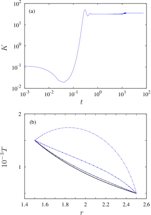
Figure 1: (a) Time series of the volume-averaged kinetic energy $K$ at ${\rm Ra}=6.2\times 10^{3}$ and ${\rm Ra}_{n}=10^{18}$. The initial condition corresponds to ${\rm Ra}=6.2\times 10^{3}$ and ${\rm Ra}_{n}=0$. From a purely differentially heated convective flow and after a long transient ($t>20$) the burning flow attractor is reached (b) Conductive temperature $T$ versus radial coordinate $r$. The bottom curve corresponds to ${\rm Ra}_{n}=0$ with $T=T_{c}$ given by Eq. 10 (differentially heated conductive state). From bottom to top, the remaining curves correspond to ${\rm Ra}_{n}=10^{11},10^{12},10^{13}$, all with ${\rm Ra}=10^{3}$.

Because ${\rm Ra}=-10^{3},10^{0},10^{1},10^{2},10^{3}<{\rm Ra}_{c}$ and ${\rm Ra}_{n}=0$ the conductive state given by Eq. 10 is stable and thus any velocity field perturbation decays to zero. By increasing ${\rm Ra}_{n}>0$ the burning conductive state, which is also spherically symmetric, is obtained. Its radial profile is shown in Fig. 1(b) for ${\rm Ra}=10^{3}$ and ${\rm Ra}_{n}=10^{11},10^{12},10^{13}$. For ${\rm Ra}_{n}<10^{11}$ the radial profile of the burning conductive state is very similar to that of the nonburning case. This indicates that very large ${\rm Ra}_{n}$ is required for convective onset. As will be shown in Sec. IV, large ${\rm Ra}_{n}$ are likely to occur in burning stellar regions. From ${\rm Ra}>10^{12}$ the radial profile is significantly different to that of ${\rm Ra}_{n}=0$, with an absolute maximum of temperature close to the middle of the shell and very large (modulus) derivatives close to the boundaries. This is similar to the conductive profile ($\propto r^{2}$) obtained when constant internal heating is considered Chandrasekhar (1981).

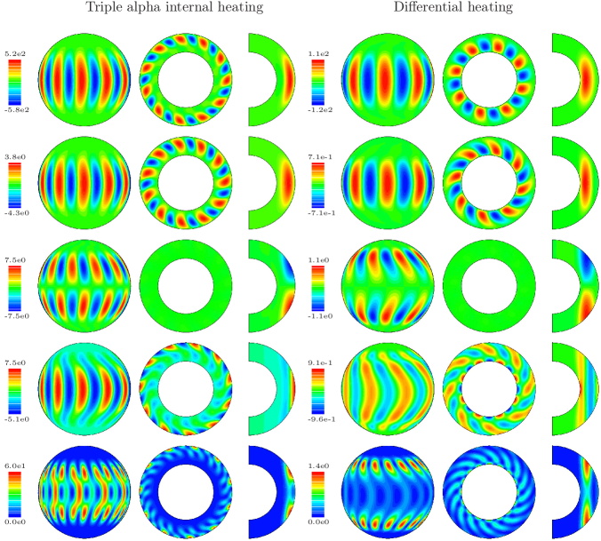
Figure 2: First row: The left three plots are the spherical, equatorial and meridional cross-sections of the contour plots of the nonaxisymmetric component of the temperature $T$ at ${\rm Ra}=6.2\times 10^{3}$ and ${\rm Ra}_{n}=10^{17}$. Right three plots: As the left, but for ${\rm Ra}=6.2\times 10^{3}$ and ${\rm Ra}_{n}=0$. The second to fifth rows show $v_{r}$, $v_{\theta}$, $v_{\varphi}$ and ${\mathbf{v}}^{2}/2$, from top to bottom. All meridional cross-sections are selected at a relative maximum. The spherical cross-sections of $v_{\theta}$, $v_{\varphi}$ and ${\mathbf{v}}^{2}/2$ are taken at the outer boundary. All of them cut a relative maximum except for $v_{\varphi}$ and ${\rm Ra}_{n}=0$ where the maximum is close to the inner boundary. The spherical cross-sections for $T$ and $v_{r}$ pass through the maximum, which is located inside the shell.

For sufficiently large ${\rm Ra}_{n}$, and each different ${\rm Ra}=-10^{3},10^{0},10^{1},10^{2},10^{3}<{\rm Ra}_{c}$ explored, the spherically symmetric burning conductive state becomes unstable to nonaxisymmetric perturbations, giving rise to waves which drift azimuthally in the prograde direction as in the case when ${\rm Ra}_{n}=0$. In all cases, the critical burning Rayleigh number required for convective onset is of order ${\rm Ra}_{n}^{c}\sim 10^{17}$, with critical azimuthal wave numbers $m_{c}\sim 10$ and critical drift frequencies $\omega_{c}\sim-50$. For instance, at ${\rm Ra}=-10^{3}$ and ${\rm Ra}_{n}=10^{18}$ an $m=10$ RW with $\omega=71.5$ is found, and at ${\rm Ra}=10^{3}$ and ${\rm Ra}_{n}=1.3\times 10^{17}$ the RW has azimuthal symmetry $m=11$ and $\omega=48.9$. These values should not differ so much from the critical values, because at ${\rm Ra}_{n}=10^{17}$ the conductive state is found to be stable. These results suggest that the ${\rm Ra}_{n}^{c}$ required for the onset of burning convection depends on the particular ${\rm Ra}$ chosen, and thus on the temperature difference between the boundaries.

By increasing ${\rm Ra}_{n}$ up to $10^{12}$, and integrating the equations, starting from the differentially heated nonburning initial condition (RW, $m=8$) but also from random fields, the same solution (RW, $m=8$) is obtained. Beyond ${\rm Ra}_{n}=10^{12}$ this Rossby wave is progressively lost (decreasing the magnitude of the velocity field) and at ${\rm Ra}_{n}\in[10^{14},10^{16}]$ the burning conductive state becomes stable again. The latter observation means that in convective systems with internal heat sources, the onset of differentially heated convection (measured by ${\rm Ra}_{c}$) depends on the internal heating rate (measured by ${\rm Ra}_{n}$). A reasonable physical interpretation of this restabilization is as follows: because ${\rm Ra}=6.2\times 10^{3}$ is very close to the onset the heat flux is almost conductive, giving a temperature profile similar to the solid black line in Fig. 1(b); by increasing ${\rm Ra}_{n}$ temperature profiles become more parabolic-like with heat flux larger at the outer boundary. In between, there exist some ${\rm Ra}_{n}$ for which heat flux is rather uniform in the fluid layer (small dashed curve of Fig. 1(b)) making difficult to excite convective motions.

At ${\rm Ra}_{n}=10^{17}$ neither the burning conductive state nor the thermal $m=8$ RW are found. The solution, which is also a RW with $m=11$ and $\omega=55.1$, is quite different from the thermal wave found previously. At ${\rm Ra}_{n}=10^{18}$ the same type of RW, with azimuthal symmetry $m=9$ and $\omega=74.6$, is obtained after a long transient (see Fig. 1(a)). These waves, driven by triple alpha heating, are of the same type as that seen at ${\rm Ra}<{\rm Ra}_{c}$ and ${\rm Ra}_{n}\gtrsim 10^{17}$ .

The comparison of the flow patterns between the triple alpha and differential heating case is shown in Fig. 2. The latter displays the contour plots of the nonaxisymmetric component of the temperature $T$, radial velocity $v_{r}$, colatitudinal velocity $v_{\theta}$, azimuthal velocity $v_{\varphi}$ and kinetic energy density ${\mathbf{v}}^{2}/2$ from top to bottom row, respectively, in spherical, meridional and equatorial cross-sections (see figure caption). The left group of three cross-sections corresponds to the triple alpha heating $m=11$ RW (at ${\rm Ra}=6.2\times 10^{3}$ and ${\rm Ra}_{n}=10^{17}$) while the right group corresponds to the thermal (Rossby) $m=8$ RW (at ${\rm Ra}=6.2\times 10^{3}$ and ${\rm Ra}_{n}=0$). Thermal (Rossby) waves characteristic of $\Pr=1$ have been widely described before for differential as well as internal heating models Zhang (1992); Simitev and Busse (2003); Garcia et al. (2018) so we comment on these only briefly. These modes have been named spiralling columnar (SC) because the flow is aligned with the rotation axis, forming convective columns that are tangential (or nearly so) to the inner cylinder (see right group of plots in Fig 2). In contrast, convection in triple alpha heating modes is attached to the outer sphere and reaches lower latitudes including the equator, similar to the equatorially attached EA modes characteristic of lower $\Pr<1$ which are more localised at equatorial latitudes Zhang (1993, 1994); Garcia et al. (2018). Triple alpha convective modes also exhibit weak vertical dependence because of the Taylor-Proudman constraint Pedlosky (1979), given the moderate, but sufficiently large, Taylor number ${\rm Ta}=2\times 10^{5}$.

III.1.2 Oscillatory burning convection

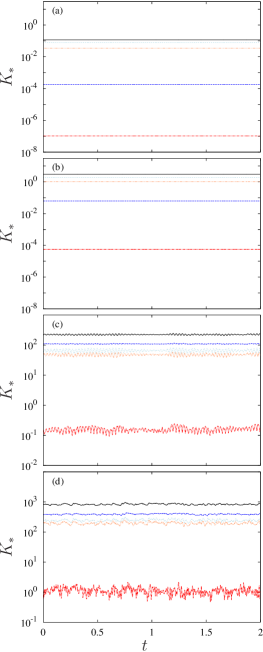
Figure 3: Time series of the kinetic energies $K$, $K_{a}^{T}$, $K_{na}^{T}$, $K_{a}^{P}$, and $K_{na}^{P}$ with solid, dashed (blue online), dotted (light-blue online), dashed-dotted (red online), and dashed-double-dotted (light-red online) line style, respectively. The parameters are ${\rm Ra}=6.2\times 10^{3}$ and (a) ${\rm Ra}_{n}=0$, (b) ${\rm Ra}_{n}=10^{17}$, (c) ${\rm Ra}_{n}=10^{19}$ and (c) ${\rm Ra}_{n}=10^{20}$.

The time series of the volume-averaged kinetic energy density $K$, and its different components $K_{a}^{T}$, $K_{na}^{T}$, $K_{a}^{P}$, and $K_{na}^{P}$ displayed in Fig. 3(a,b) correspond to the thermal $m=8$ RW at ${\rm Ra}=6.2\times 10^{3}$ and the burning $m=11$ RW at ${\rm Ra}=6.2\times 10^{3}$ and ${\rm Ra}_{n}=10^{17}$. They are constant because azimuthally averaged properties do not change with time, as the flow drifts in that direction. Both solutions have stronger toroidal components and are almost nonaxisymmetric $K_{a}^{P}<K_{a}^{T}<K_{na}^{P}<K_{na}^{T}$ because they are very close to the respective onset. Increasing ${\rm Ra}_{n}$ results in a strong relative increase of zonal motions measured by $K_{a}^{T}$, giving $K_{a}^{P}<K_{a}^{T}\approx K_{na}^{P}<K_{na}^{T}$ at ${\rm Ra}_{n}=10^{18}$ (not shown in the figure) and $K_{a}^{P}<K_{na}^{P}\lesssim K_{na}^{T}<K_{a}^{T}$ at ${\rm Ra}_{n}=10^{19}$ and ${\rm Ra}_{n}=10^{20}$ (see Fig. 3(c,d)). In all cases $K_{a}^{P}<10^{-3}K$, meaning that the axisymmetric component is almost purely toroidal. The time series of Fig. 3(c,d) exhibits oscillatory and chaotic dependence with a strong axisymmetric and toroidal component (zonal wind). All of these features of convection are typical with stress-free boundary conditions, and have been reported before with internal heating sources Simitev and Busse (2003) as well as externally forced temperature gradients Christensen (2002). The description of their flow patterns is delayed to Sec. III.2.3, where turbulent solutions will be also detailed.

Figure 4: Time series of the temperature at $r=r_{i}+0.5d$, $\varphi=0$ and three different colatitudes $\theta=3\pi/8$, $\theta=\pi/4$ and $\theta=\pi/8$, with solid (black online), dashed (blue online), dotted (light-blue online) line style, respectively. The parameters are ${\rm Ra}=6.2\times 10^{3}$ and (a) ${\rm Ra}_{n}=0$, (b) ${\rm Ra}_{n}=10^{17}$, (c) ${\rm Ra}_{n}=10^{19}$ and (c) ${\rm Ra}_{n}=10^{20}$.

The time series of the temperature measured in the middle of the shell ($r=r_{i}+0.5d$) at $\varphi=0$ and three different colatitudes, evenly distributed between the equatorial plane and the north pole $\theta=\pi/8$, $\theta=\pi/4$ and $\theta=3\pi/8$ are displayed in Fig. 4(a,b,c,d) for the same solutions as Fig. 3(a,b,c,d), respectively. For the $m=8$ RW at ${\rm Ra}_{n}=0$ and the $m=11$ RW at ${\rm Ra}_{n}=10^{17}$ the temperature is periodic and the amplitude of the oscilations is around $3\%$ of the mean (see Fig. 4(a,b)) meaning that these solutions represent small deviations from the conductive state. Both the amplitude of the oscillations and the mean decrease with increasing $\theta$, and the temperature in the polar regions ($\theta=\pi/8$) is almost constant (i.e conductive). With increasing ${\rm Ra}_{n}$ the amplitude of oscillations becomes larger (up to around $30\%$ at ${\rm Ra}_{n}=10^{20}$, see Fig. 4(d)) and the temperature in the polar regions becomes more oscillatory. The strongest temperature oscillations in our model of triple alpha burning convection are located near the equatorial region, which may have observational consequences. In addition, the time series of chaotic solutions shown in Fig. 4(c,d)) exhibits small rapid fluctuations, coexisting with these large oscillations which have a longer associated time scale. This longer time scale seems not to vary much with ${\rm Ra}_{n}$ and is similar to the corresponding periodic oscilations at the onset (compare Fig. 4(b) with Fig. 4(d)). A deeper study of the time scales associated with burning driven flows is considered in Sec. III.2.4.

III.2 High ${\rm Ra}_{n}$ convection and mean properties

Time averaged global and local physical properties, such as volume averaged kinetic energy densities or temperature at a point inside the shell, as well as flow patterns, are described and interpreted in the following subsection. In addition, some power laws derived from the equations of motion will be compared to the numerical results, by assuming certain force balances Gastine et al. (2016); Garcia et al. (2017). This has been shown to be a successful tool for obtaining estimations of realistic phenomena Aubert et al. (2001); Christensen (2002); Garcia et al. (2014c); Oruba and Dormy (2014b) in the geodynamo context. The analysis is restricted to ${\rm Ra}=6.2\times 10^{3}$, and comprises a large sequence of solutions, including those studied in the previous section, with increasing ${\rm Ra}_{n}$ up to $10^{27}$. This section is focused on high ${\rm Ra}_{n}$ flows and on detailing the associated physical regimes. By increasing ${\rm Ra}_{n}$, turbulent convection develops after different transitions from the laminar regime. We have found that burning driven convection shares relevant flow features with the type of convection described for planetary atmospheres Heimpel and Aurnou (2007); Aurnou et al. (2007); Gastine et al. (2013) modelled with an externally forced temperature gradient. In particular, we find the same regimes described in Gastine et al. (2013) (see the summary in their conclusions) for both Boussinesq and anelastic approximations.

Table 3 contains data that give a preliminary description of the route to turbulence occuring in triple alpha burning convection. The Rossby number, and its poloidal component measuring vigour of convective flow Christensen (2002); Garcia et al. (2014c), increase monotonically. For the small ${\rm Ra}_{n}$, $Ro\ll 1$ and $Ro_{p}\approx Ro/2$ indicates that Coriolis forces are important, and the flow is moderately convective. However, by increasing nuclear burning rate $Ro_{p}\lesssim{\rm Ro}\sim 1$, thus Coriolis forces play secondary role and the flow is strongly convective. The ratio $K/K_{na}$ helps to identify these different flow regimes Gastine et al. (2013), decreasing from ${\rm Ra}_{n}=10^{23}$ for the largest ${\rm Ra}_{n}$, and provides useful information. For instance, ${\rm K}/{\rm K}_{na}$ is also a maximum in the vicinity of ${\rm Ra}_{n}=10^{19}$, the regime of oscillatory and chaotic (but coherent) burning convection studied previously. The spherical harmonic order $m_{\text{max}}$, in which $\max K_{m}$ is reached, or equivalently $l_{\text{max}}$ for the spherical harmonic degree, are often used for estimating length scales present in the system. More accurate estimations could be obtained with with $(\overline{n})^{-1}$ Christensen and Aubert (2006) (or $(\overline{n_{p}})^{-1}$ for convective length scales). This table points to so-called Rossby-wave turbulence, i.e the low wave number route to chaos (see Ruelle and Takens (1971); Eckmann (1981) for examples of routes) in which the energy is contained at successively lower wave numbers when increasing the forcing (inverse cascade, because of the shearing produced by differential rotation Schaeffer and Cardin (2005)). Regarding the regimes in the extremes (rotating waves at ${\rm Ra}_{n}=10^{17},10^{18}$ or the most turbulent solutions from ${\rm Ra}_{n}\geq 10^{25}$), large length scales that do not change substantially are found, and the convective flow develops smaller scale structures.

$$\begin{array}[]{lccccccccccc}\hline\cr{\rm Ra}_{n}&\overline{Ro}&\overline{Ro_{p}}&\overline{K/K_{na}}&m_{\text{max}}&l_{\text{max}}&\overline{n}&\overline{n_{p}}\\ \hline\cr 0&0.001&0.0006&1.002&8,0,16&9,11,3&9.44&8.31\\ 10^{17}&0.006&0.003&1.02&11,0,22&12,14,3&11.70&11.14\\ 10^{18}&0.019&0.010&1.32&9,0,18&10,3,1&8.46&9.62\\ 10^{19}&0.047&0.022&1.97&0,8,16&3,1,9&8.47&14.67\\ 10^{20}&0.091&0.044&1.89&0,5,10&3,1,5&8.09&13.63\\ 10^{21}&0.17&0.101&1.20&1,0,3&3,9,12&9.64&12.69\\ 10^{22}&0.32&0.16&2.53&0,2,5&3,1,5&7.06&14.92\\ 10^{23}&0.50&0.25&2.88&0,2,4&3,1,7&7.06&15.81\\ 10^{24}&0.68&0.35&2.74&0,2&3,1,5&8.19&17.41\\ 10^{25}&0.81&0.48&2.06&0,2&3,1,5&11.28&19.52\\ 10^{26}&0.92&0.64&1.50&0,5&3,1,5&16.09&21.40\\ 10^{27}&1.10&0.84&1.20&0,5&1,3,6&21.23&23.07\\ \hline\cr\end{array}$$

Table 3: Burning Rayleigh number ${\rm Ra}_{n}$, mean Rossby and poloidal Rossby numbers, $\overline{Ro}$ and $\overline{Ro_{p}}$, mean ratio of the total to the nonaxisymmetric KEDs, $\overline{K/K_{na}}$, leading azimuthal wave numbers having a relative maximum of $\overline{K_{m}}$ (the KED considering a single wave number $m$), leading spherical harmonic degrees having a relative maximum of $\overline{K_{l}}$ and time averaged mean total and poloidal spherical harmonic degree $\overline{n}$ and $\overline{n_{p}}$.

III.2.1 Time-averaged Properties

The different flow regimes distinguished in Table 3 are investigated with the help of time averages displayed in Fig. 5 and Fig. 6. The former examines the volume averages of the different components of the kinetic energy density or the volume averaged force balance, but also temperature recorded at different points inside the shell. The latter analyses the zonal flow also at different colatitude and radial positions (see figure captions). In the left region of both figures (up to ${\rm Ra}_{n}=10^{12}$) the plotted variables are constant and equal to those corresponding to the differentially heated nonburning solution at ${\rm Ra}_{n}=0$. As mentioned in the previous section, at ${\rm Ra}_{n}=10^{13}$ the imposed temperature gradient becomes less efficient at maintaining convection, and the kinetic energy density of the solution decreases. At ${\rm Ra}_{n}=10^{14},10^{15},10^{16}$ convection is no longer sustained, and the triple alpha conductive state is recovered. This is why these points are missing in the plots.

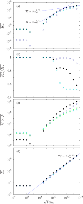
Figure 5: Physical properties versus $\sqrt{{\rm Ra}_{n}}$: (a) Time-averaged global (volume-averaged) kinetic energies $K$ ($\bullet$), $K_{a}$ ($\circ$) and $K_{na}$ ($\ast$). The fitting lines are $\overline{K}=8\times 10^{-8}{\rm Ra}_{n}^{1/2}$ and $\overline{K}=5\times 10^{1}{\rm Ra}_{n}^{1/8}$. (b) Ratios of the time-averaged equatorially symmetric over global kinetic energies $K^{s}/K$ ($\bullet$), $K_{a}^{s}/K_{a}$ ($\circ$) and $K_{na}^{s}/K_{na}$ ($\ast$). (c) Time-averaged rms curl of forces integrals $\mathcal{\nabla\times F}_{I}$ ($\bullet$, Inertial), $\mathcal{\nabla\times F}_{V}$ ($\circ$, viscous) and $\mathcal{\nabla\times F}_{C}$ ($\ast$, Coriolis). (d) Time-averaged temperatures $\bar{T_{1}}$, $\bar{T_{2}}$ and $\bar{T_{3}}$ taken at $\varphi=0$, $\theta=3\pi/8$ and $r=r_{1}=r_{i}+0.15d$ ($\ast$), $r=r_{2}=r_{i}+0.5d$ ($\circ$) and $r=r_{3}=r_{i}+0.85d$ ($\bullet$), respectively (where $d=r_{o}-r_{i}$). The fitting line corresponds to $\overline{T_{2}}=(1.95\pm 0.15){\rm Ra}_{n}^{0.223\pm 0.001}$.

In the first burning convective regime, $10^{17}\leq{\rm Ra}_{n}\leq 10^{19}$, corresponding to oscillatory solutions (regime I of Gastine et al. (2013)), the zonal component of the flow grows rapidly (see Fig. 5(a)) and Coriolis forces are still important (see Fig. 5(c)), helping to maintain the equatorial symmetry of the flow (see Fig. 5(b)). Zonal circulations are positive near the outer and negative near the inner boundaries (see Fig. 6(c)). This also occurs at ${\rm Ra}_{n}=10^{20},10^{21}$ but these solutions are different because the equatorial symmetry has been broken, the Coriolis forces start to be of second order (see Fig. 5(b) and Fig. 5(c)), and the axisymmetric flow component starts to decrease (see table 3). These solutions belong to a transition regime across which the structure of the mean zonal flow is strongly changed. A very similar regime was also found in Gastine et al. (2013) (where it was called the transitional regime), but only for strongly stratified anelastic models. According to Gastine et al. (2013), because of the strong stratification, different force balances are achieved at different depths in the shell. In this regime buoyancy dominates near the outer boundary while the Coriolis force is still relevant in the deep interior. This reduces the amplitude of the zonal flow and leads to a characteristic dimple in the center of the equatorial jet Gastine et al. (2013). As will be shown in Sec. III.2.3 the signature of this dimple is also present in our unstratified models.

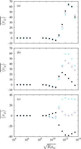
Figure 6: Time-averaged mean zonal flow (azimuthally-averaged $v_{\varphi}$) versus $\sqrt{{\rm Ra}_{n}}$: At colatitude (a) $\theta=\pi/8$, (b) $\theta=\pi/4$ and (c) $\theta=3\pi/8$. The symbols indicate the radial position: ($\ast$) $r=r_{1}=r_{i}+0.15d$, ($\circ$) $r=r_{2}=r_{i}+0.5d$ and ($\bullet$) $r=r_{3}=r_{i}+0.85d$ (where $r_{i}=1.5$ and $r_{o}=2$).

The second regime (also regime II in Gastine et al. (2013)) corresponds to flows ($10^{22}\leq{\rm Ra}_{n}\leq 10^{24}$) which have the maximum zonal component (see table 3). These solutions are characterised by large scale convective cells, volume-averaged kinetic energy growing as ${\rm Ra}_{n}^{1/2}$, and inertial forces becoming more relevant with respect to Coriolis and viscous forces. In contrast to the previous regime the zonal flow pattern is reversed and becomes negative near the outer boundary and positive near the inner. In this regime, the positive mean zonal flow near the inner boundary is strongly increased at mid and high but also close to equatorial latitudes. In these latitudes the positive mean zonal flow is weaker. The radial dependence is enhanced with increasing latitude. In addition, although equatorial symmetry of the nonaxisymmetric flow is clearly broken, this is not the case of the axisymmetric (zonal) flow.

A third regime (also regime III in Gastine et al. (2013)) is obtained for the largest ${\rm Ra}_{n}\geq 10^{25}$ explored, corresponding to strongly convective and nonaxisymmetric turbulent flows. In this regime the balance seems to be between inertial and viscous forces, with volume-averaged kinetic energy slowly growing as ${\rm Ra}_{n}^{1/8}$, and the volume averaged zonal component of the flow starting to slowly lose equatorial symmetry, while remaining roughly constant. The change of tendency of the axisymmetric component of the flow is also local, as can be observed in Fig. 6. Whilst in equatorial regions the zonal flow remains roughly constant, at higher latitudes it decreases quite sharply, which may be indicative of the progressive loss of equatorial symmetry. In the case of the nonaxisymmetric flow, its equatorially symmetric and antisymmetric components are balanced, as reflected by the constant ratio $K^{s}_{na}/K_{na}\approx 0.5$. A fourth regime can be guessed by looking Fig. 5(b). It will correspond to fully isotropic turbulence characterized by nearly equal equatorially symmetric and antisymmetric components of the zonal flow ($\overline{K^{s}_{a}}/\overline{K_{a}}\approx 0.5$).

III.2.2 Force Balance

For all the ${\rm Ra}_{n}$ explored, the time averages of the temperature are quite similar inside the shell (Fig. 5(d)). The latter figure shows that mean temperatures are slightly larger close to the outer boundary, except for the turbulent solutions where the radial dependence seems to disappear. Mean temperatures close to the equatorial region in the middle of shell grow as $\overline{T}=(1.95\pm 0.15){\rm Ra}_{n}^{0.223\pm 10^{-3}}$ and thus the different flow regimes cannot be clearly identified. Notice that the latter scaling is better satisfied at the largest ${\rm Ra}_{n}$. For smaller forcing ${\rm Ra}_{n}\leq 10^{23}$, the exponent of the power law is a little bit larger, around $0.24\approx 1/4$. As argued in the following this exponent, and ${\rm Ra}_{n}^{1/2}$ and ${\rm Ra}_{n}^{1/8}$ found for the kinetic energy density, can be deduced from the equations. The results are compared with Gastine et al. (2016), a very exhaustive and recent study about scaling regimes in spherical shell rotating convection.

Assuming that in the energy equation (Eq. 8) the internal triple-alpha heat generation is balanced with the temperature Laplacian $\nabla^{2}T\sim{\rm Ra}_{n}T^{-3}e^{-{\rm B}_{n}/T}$, the characteristic length scale remains roughly constant (of the same order) with ${\rm Ra}_{n}$ (see Table 3), and $T\sim{\rm Ra}_{n}^{\xi}$ with $\xi>0$ gives ${\rm Ra}_{n}^{\xi}\sim{\rm Ra}_{n}^{(1-3\xi)}$, because if ${\rm Ra}_{n}$ is large the term $e^{-{\rm B}_{n}/T}\sim e^{-{\rm B}_{n}/{\rm Ra}_{n}^{\xi}}\sim 1$. Then $\xi\approx 1/4$, in very good agreement with our results. In addition, for ${\rm Ra}_{n}\leq 10^{23}$ we have found from the simulations $\overline{K}\sim{\rm Ra}_{n}^{1/2}$, i.e $U\sim{\rm Ra}_{n}^{1/4}$ with $U$ being the characteristic velocity of the fluid. When viscous and Coriolis forces are balanced with the Archimedes (buoyancy) force in the momentum equation (the so-called VAC balance, see Gastine et al. (2016) and references therein), as Fig. 5(c) suggests, and with the previous assumptions for the length scales, the characteristic velocity is $U\sim T\sim{\rm Ra}_{n}^{1/4}$.

When the VAC balance is lost for the turbulent solutions ${\rm Ra}_{n}\gtrsim 10^{24}$, a new power law $\overline{K}\sim{\rm Ra}_{n}^{1/8}$, i.e $U\sim{\rm Ra}_{n}^{1/16}$, is obtained. This very low exponent may be explained by again making use of the energy equation and assuming that its inertial term starts to play a role, giving rise to a new balance. The length scales for the temperature $L$ are no longer constant, modifying slightly the $\nabla^{2}T\sim{\rm Ra}_{n}T^{-3}e^{-{\rm B}_{n}/T}$ balance to $T/L^{2}\sim{\rm Ra}_{n}T^{-3}$. Because the solutions have very large velocities we may assume ${\mathbf{v}}\cdot\nabla T\sim{\rm Ra}_{n}T^{-3}e^{-{\rm B}_{n}/T}$, i.e, $UT/L\sim{\rm Ra}_{n}T^{-3}$ and thus $UT/L\sim T/L^{2}$ or equivalently $UL\sim 1$. If $T\sim{\rm Ra}_{n}^{\xi}$ and $U\sim{\rm Ra}_{n}^{\zeta}$ then $\zeta=(1-4\xi)/2$ which is in close agreement with our results. With $\xi=0.22$ we obtain $\zeta=0.06\approx 1/16$.

Very similar scaling regimes have been reported previously in the context of differentially heated convection Gastine et al. (2016). They are the weakly non-linear regime (VAC balance) and the non-rotating regime (IA balance). This may be an indication that very similar mechanisms govern both differentially or internally heated systems, even in the case of temperature dependent internal sources.

III.2.3 Triple-alpha Convective Patterns

The variation of the topology of the flow with increasing ${\rm Ra}_{n}=10^{20},10^{21},10^{22},10^{23},10^{26},10^{27}$, i.e the patterns of triple alpha convection, can be analysed with the help of Fig. 7 and Fig. 8. The former displays the contour plots of the temperature (with increasing ${\rm Ra}_{n}$ from top to bottom rows) in spherical, equatorial and meridional cross-sections (left group of plots), as well as those for the azimuthal velocity (right group of plots). The latter compares the total kinetic energy of the flow (first row) with the axisymmetric component of the azimuthal velocity (second row) on meridional cross-sections for the same sequence of ${\rm Ra}_{n}$ as Fig. 7. As usual, spherical and meridional cross-sections pass through a relative maximum. The azimuthally averaged azimuthal velocity contour plots shown in the second row of Fig. 8 can be easily compared with Figure 2 of Gastine et al. (2013), showing a good agreement.

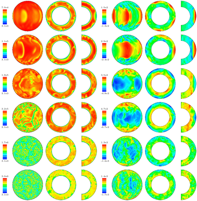
Figure 7: Instantaneous contour plots at ${\rm Ra}_{n}=10^{20},10^{21},10^{22},10^{23},10^{26},10^{27}$ (from top row to bottom row). The left three plots are the spherical, equatorial and meridional cross-sections of the temperature $T$. Right three plots: Same cross-sections for $v_{\phi}$. Meridional cross-sections and the spherical cross-section of $T$ are taken at a relative maximum. The spherical cross-section of $v_{\phi}$ is at the outer surface.

Figure 8: Instantaneous contour plots at ${\rm Ra}_{n}=10^{20},10^{21},10^{22},10^{23},10^{26},10^{27}$ (from left to right) showing the meridional cross-sections of the kinetic energy density ${\mathbf{v}}^{2}/2$ (1st row) and the mean zonal flow (azimuthally-averaged $v_{\varphi}$) (2nd row). Cross-sections of ${\mathbf{v}}^{2}/2$ pass through a maximum.

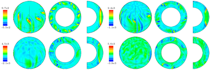
Figure 9: Instantaneous contour plots at ${\rm Ra}=6.2\times 10^{3}$ and ${\rm Ra}_{n}=10^{19},10^{20},10^{21},10^{22}$ (from left to right and from top to bottom group of plots). Each group of three plots are the spherical, equatorial and meridional cross-sections of the axial vorticity $w_{z}$. Spherical cross-sections are taken at $r=r_{i}+0.95d$, $r=r_{i}+0.8d$, $r=r_{i}+0.3d$ and $r=r_{i}+0.5d$ for ${\rm Ra}_{n}=10^{19},10^{20},10^{21},10^{22}$, respectively. Meridional cross-sections are taken where $w_{z}$ has a relative maximum.

At ${\rm Ra}_{n}=10^{20}$ the solutions belong to the oscillatory regime. Temperature is maximum in the polar regions and almost conductive (see spherical cross-section). A remarkable characteristic of the burning convection is that large azimuthally elongated outward plumes coexist with very narrow inward cold cells. The outward plumes are mushroom like and correspond to a large outward radial flow. At lower latitudes, close to the equatorial region, an $m=5$ convective pattern develops (see equatorial cross-section). This $m=5$ pattern is clearly distinguished in the contour plots of $v_{\varphi}$. There is an equatorial belt of positive zonal circulation attached to the outer boundary. At higher latitudes the zonal circulation is strongly negative, decreasing its amplitude up to the poles. The total kinetic energy density, see meridional cross-section shown in Fig. 8 (first row, left), is maximum just where the negative circulation takes place, while the axisymmetric azimuthal velocity (Fig. 8 second row, left) is maximum at the positive equatorial belt. This figure reveals also the strong equatorial symmetry of the flow.

Very narrow downwelling plumes, elongated in the colatitude direction, are clearly observed on the equatorial region at ${\rm Ra}_{n}=10^{21}$ as Coriolis forces are still noticeable (see temperature spherical cross-sections of Fig. 7). Colatitude directed coherent vortices have been also obtained in Boussinesq (Fig. 4 of Heimpel and Aurnou (2012)) or anelastic (Fig. 6 of Brown et al. (2008)) models, in the contexts of Saturn’s atmosphere and solar convection, respectively. The latter models considered differential heating in a regime strongly influenced by rotation. We note however the very different azimuthal and radial nature of our coherent vortices when considering an additional source of internal heating. The flow patterns at ${\rm Ra}_{n}=10^{21}$ are similar as those at ${\rm Ra}_{n}=10^{20}$ but with a weaker zonal component (see 2nd plot, 2nd row of Fig. 8). The positive equatorial belt has been disrupted, becoming a large convective cell in which the kinetic energy is concentrated (see 2nd plot, 1st row of Fig. 8). The flow then has strong azimuthal symmetry $m=1$ (see the equatorial cross-sections of Fig. 8 and table 3). Convection is spreading to high latitudes, and polar zonal circulations become important (see 2nd plot, 2nd row of Fig. 8). The flow is still equatorially symmetric ($K_{s}>0.8K$) but antisymmetric motions increase noticeably when compared with solutions at lower ${\rm Ra}_{n}$. The dimple seen in the equatorial belt of zonal motions (see 2nd plot, 2nd row of Fig. 8) was associated in Gastine et al. (2013) with a transitional regime. As we argue at the end of this section, this regime seems also be valid in our case.

The corresponding flow topology at ${\rm Ra}_{n}=10^{22},10^{23}$ is quite different from that at lower ${\rm Ra}_{n}$. While large scale temperature vortices are still present, convection is more vigorous and more developed, with small scale motions in the polar regions. The meridional and latitudinal extent of the convective cells is starting to decrease (see spherical cross-sections of $T$) while it remains large (similar to the gap width) in the radial direction (see equatorial cross-sections of $T$). This gives more support to our assumption of a characteristic length scale of order unity when deriving the corresponding temperature and velocity scalings in Sec. III.2.2. As stated, when studying time averaged properties from ${\rm Ra}_{n}\geq 10^{22}$, the flow pattern has reversed and now the circulation occurring in the equatorial belt is negative whilst at higher latitudes it is positive. The meridional extension of the equatorial belt decreases, and the motions are more attached to the outer surface (see 3nd/4th plot, 1st and 2nd row of Fig. 8). While the axisymmetric flow (and thus the equatorial belt) is still equatorially symmetric, this symmetry is progressively lost on the rest of the shell. When comparing to the corresponding differentially heated Boussinesq models of Fig. 2 in Gastine et al. (2013), our models exhibit larger steady axially oriented regions (green color), which tend to spread to larger latitudes, i.e moving radially inwards, with increasing ${\rm Ra}_{n}$.

The two most extreme cases at ${\rm Ra}_{n}=10^{26},10^{27}$ exhibit very fine temperature structures close to the outer boundary, and of granular type like those observed on the Sun’s surface. Nevertheless, the large scale weak temperature vortices still recall the topology of the triple alpha conductive state. The negative and positive circulations become more nonaxisymmetric, the latter nearly reaching the poles. Although the number of small scale structures is increasing, negative azimuthal velocity cells, elongated on the meridional direction, are still present on equatorial latitudes even at ${\rm Ra}_{n}=10^{27}$. In the latter case, these negative meridional cells alternate with very thin positive plumes that connect positive circulations of both poles (see spherical cross-section of $v_{\varphi}$). Although motions are concentrated very close to the outer boundary (see rightmost plots, 1st row of Fig. 8), they are no longer located near equatorial latitudes and may reach high latitudes. In addition the equatorial symmetry of the flow is clearly lost, although not that of its axisymmetric component (see also rightmost plots, 2nd row of Fig. 8). The latter is stronger at high latitudes, in contrast to what happens at lower ${\rm Ra}_{n}$.

The typical anelastic transitional flows of Gastine et al. (2013) exhibit quasigeostrophic structures in the interior of the shell, whilst they are more buoyancy dominated (radially aligned) near the outer boundary. The critical radial distance, $r_{\text{mix}}$ in Gastine et al. (2013), separating the two dynamical behaviours within the shell increases (from the outer boundary to the inner) with the forcing. This also occurs in our Boussinesq models, as shown in Fig. 9, but with different patterns which are due to the different forcing mechanisms (differentially heated anelastic versus triple-alpha internal heating) of the convection. The figure displays the contour plots of the axial vorticity $w_{z}$ on spherical, meridional and equatorial cross-sections (the latter are shown in Fig. 13 of  Gastine et al. (2013) for three anelastic models). The positions of the cross-sections are displayed with black lines in the contour plots. Four representative solutions belonging to regimes I, transitional, and II, at ${\rm Ra}_{n}=10^{19},10^{20},10^{21},10^{22}$, are shown. In regime I the flow is quasigeostrophic outside the tangent cylinder while convection is absent in the inner region (see left top group of plots). At ${\rm Ra}_{n}=10^{20}$, a rough critical radius $r_{\text{mix}}=r_{i}+0.8d$ can be identified (see right top group of plots, equatorial and meridional cross-sections), becoming larger $r_{\text{mix}}=r_{i}+0.3d$ at ${\rm Ra}_{n}=10^{21}$ (see left bottom group of plots). In agreement with Gastine et al. (2013), for $r>r_{\text{mix}}$ vorticity is radially aligned (best seen in the meridional cross-sections) while for $r<r_{\text{mix}}$ the quasigeostrophic columns can be identified. However, in contrast to Gastine et al. (2013) this behaviour is more evident in the polar regions (see spherical cross-sections) than at lower latitudes where axially aligned structures at $r>r_{\text{mix}}$ still survive. For flows belonging to regime II small convective structures within all $r$ can be found (see right bottom group of plots) but they are now quite aligned in the vertical direction because the negative zonal circulations at low latitudes are becoming stronger.

$$\begin{array}[]{lcccccccccccc}\hline\cr{\rm Ra}_{n}&f^{T}_{\text{max}}&[f^{T}_{1},f^{T}_{2}]&\overline{f^{T}}&f^{v_{\varphi}}_{\text{max}}&[f^{v_{\varphi}}_{1},f^{v_{\varphi}}_{2}]&\overline{f^{v_{\varphi}}}&f^{\langle v_{\varphi}\rangle}_{\text{max}}&[f^{\langle v_{\varphi}\rangle}_{1},f^{\langle v_{\varphi}\rangle}_{2}]&\overline{f^{\langle v_{\varphi}\rangle}}\\ \hline\cr 10^{17}&8.77&[8.77,80.0]&9.21&8.77&[8.77,80.0]&10.6&--&--&--\\ 10^{18}&11.8&[11.8,59.1]&14.8&11.8&[11.8,71.2]&15.0&--&--&--\\ 10^{19}&21.0&[2.50,31.0]&15.9&21.0&[5.29,41.9]&22.1&34.57&[1.23,45.0]&25.2\\ 10^{20}&28.2&[2.17,39.6]&24.4&28.2&[2.54,56.3]&26.5&8.881&[0.73,52.1]&32.8\\ 10^{21}&16.1&[3.81,60.3]&61.1&12.7&[7.00,66.4]&30.1&6.44&[1.99,55.9]&45.8\\ 10^{22}&26.0&[14.7,91.1]&171&12.5&[2.03,57.2]&71.2&2.38&[7.52,80.4]&49.7\\ 10^{23}&16.7&[16.7,235]&345&4.58&[4.58,56.5]&38.4&2.48&[2.48,90.2]&111\\ 10^{24}&82.8&[25.1,287]&375&45.6&[4.22,102]&90.5&31.53&[18.0,66.2]&35.0\\ 10^{25}&54.3&[23.8,360]&270&17.4&[13.9,128]&180&33.80&[5.62,115]&50.5\\ 10^{26}&110&[16.8,372]&402&91.8&[6.70,252]&377&19.91&[19.9,164]&179\\ 10^{27}&42.3&[16.9,509]&948&35.3&[14.1,350]&233&47.48&[10.6,231]&198\\ \hline\cr\end{array}$$

Table 4: Burning Rayleigh number ${\rm Ra}_{n}$, the frequency with larger amplitude $f^{*}_{\text{max}}$, the interval $[f^{*}_{1},f^{*}_{2}]$ containing the 10 first frequencies with larger amplitude, and mean frequency $\overline{f^{*}}$ of the frequency spectrum of temperature $T$, azimuthal velocity $v_{\varphi}$ and zonal flow $\langle v_{\varphi}\rangle$ taken close to the outer boundary and the equatorial plane (at $(r,\theta,\varphi)=(r_{i}+0.85d,3\pi/8,0)$).

III.2.4 Flow Time Scales

It is interesting to address which are the relevant time scales present in the different flow regimes obtained with the DNS. Table 4 lists the frequency with larger amplitude $f^{*}_{\text{max}}$, the interval $[f^{*}_{1},f^{*}_{2}]$ containing the 10 first frequencies with larger amplitude, and the mean frequency $\overline{f^{*}}$ of the frequency spectrum of temperature $T$, azimuthal velocity $v_{\varphi}$ and zonal flow $\langle v_{\varphi}\rangle$ taken close to the outer boundary and the equatorial plane (at $(r,\theta,\varphi)=(r_{i}+0.85d,3\pi/8,0)$). Rotating waves (${\rm Ra}_{n}=10^{17},10^{18}$) close to the onset have time scales quite similar to the critical frequencies $2\pi/\omega_{c}\sim 10$. Usually secondary bifurcations giving rise to oscillatory flows involve large time scales, as is the case for ${\rm Ra}_{n}=10^{19},10^{20}$, with relevant frequencies $f\sim 1$.

With increasing ${\rm Ra}_{n}\geq 10^{21}$, time scales that are several orders of magnitude smaller become important, but nonetheless larger time scale similar to those at the onset remain relevant: while $f^{*}_{1}\sim 10$ remains quite constant $f^{*}_{2}\sim 10^{2}$ increases, but not too much. This also occurs in differentially heated convection with increasing ${\rm Ra}$. Thus the study of the onset of convection is of fundamental importance, because it reveals time scales that are found to be present even at highly supercritical regimes. Going into more detail on the latter, by comparing $\overline{f^{T}}$ with $\overline{f^{v_{\varphi}}}$ we see that the flow has larger time scales than the temperature variations. This is particularly true in the case of the zonal flow having the smallest $\overline{f^{\langle v_{\varphi}\rangle}}$ which are very similar to the conditions corresponding to the onset. For instance, at $10^{19}\leq{\rm Ra}_{n}\leq 10^{25}$ time scales are $\overline{f^{\langle v_{\varphi}\rangle}}\lesssim 50,$ while at the onset they are $2\pi/\omega_{c}\approx 10$. We recall that zonal flow time scales are important because of their observational consequences.

IV Convection in Accreting Neutron Star Oceans

Before linking our results to convection occurring in accreting neutron star oceans (see the introductory section) we should stress that we are still far from realistic modelling. In such environments the flow is stratified, thus compressible convection should be considered. However, as argued in Garcia et al. (2018), Boussinesq convection constitutes the very first step towards the study of convective patterns in global domains. Some insights into the consideration of compressibility effects are provided in Gastine et al. (2013), by means of the anelastic approximation. According to this study the same I,II and III flow regimes, including the transitional regime (between I and II), are obtained with strong stratification. Retrograde zonal flow amplitudes are decreased with respect to the Boussinesq case in regime II but this seems not to happen in regime I. In addition, strongly stratified flows favour the appearance of the transitional regime, and the transition to regime III is delayed.

As mentioned before, this study is focussed primarily on the effect of increasing internal heating via triple-alpha reactions, so the values chosen for $\Pr$, ${\rm Ta}$, and $\eta$ are not extreme. In addition, in real stars the fraction of helium would deplete over time as carbon and heavier elements form - while in this study, for fixed ${\rm Ra}_{n}>0$, heat is generated continuously in the ocean. More realistic models, accounting for nuclear physics as well as hydrodynamics, would require coupling the Navier-Stokes equation, energy equation, and a nuclear reaction network; far outside the scope of this initial study.

When helium is burning steadily, (see Bildsten (1998) for details) heat generated by nuclear reactions is balanced by radiative cooling ($q_{\text{cool}}\propto T^{4}$). When this balance no longer, holds a thermal instability gives rise to a thermonuclear runaway and the associated Type-I X ray burst Bildsten (1998). In the latter paper, marginal stability curves for several accretion rates were given as a function of temperature and column depth; these calculations indicated that unstable burning (bursting) should continue up to accretion rates a factor of a few larger than the value inferred from observations. Recent studies (see Zamfir et al. (2014) and the references in the introduction) have considered an additional source of heat at the base of the ocean, to bring the critical accretion rate at which burning stabilises closer to observational values. Other studies Keek et al. (2009), based on one-zone hydrodynamic stellar evolution models, have achieved a similar effect by considering an inward diffusion of helium due to the influence of rotation and magnetic fields. In contrast to these studies, in our study nuclear heating is balanced by both thermal advection and diffusion. For the latter we are assuming constant density and thermal conductivity (Boussinesq), and any additional sink of heat is located at the upper boundary. We are thus not taking into account radiative processes but focusing on the heat convective transport on a rotating spherical shell.

There are several numerical studies (local in nature) modelling convection during bursts on accreting neutron stars (see for instance Woosley et al. (2004); Malone et al. (2011)). In the former, convection is implemented using mixing length theory, while in the latter the momentum equation (advection-like) for convective velocity is solved. These studies ( Woosley et al. (2004); Malone et al. (2011)) - but also earlier ones Weaver et al. (1978) devoted to the study of stellar evolution of massive stars - rely on the Schwarzschild and Ledoux criterion to compute the onset of convection (when thermal and compositional buoyancy overcomes gravity). In the Schwarzschild criterion an instantaneous chemical equilibrium is assumed, which favours the appearance of the convective instability Weiss et al. (2004). This means that the fluid can be Schwarzschild unstable but Ledoux stable to velocity perturbations, referred to as semiconvection in previous studies Weaver et al. (1978); Woosley et al. (2004); Malone et al. (2011). These studies (and also Weinberg et al. (2006); Yu and Weinberg (2018)) have built up the current picture of the role played by convection in the thermal evolution of a burst. Burning is mainly localised at the base of the accreted layer where temperature and density are larger. Because the burning time scale is much shorter than the time scale of radiative processes, nuclear energy is more efficiently dissipated by convection. Fluid motions spread towards the upper radiative layers of the accreted ocean until the entropy of the convective layer balances the radiative entropy. Finally, because of the decrease of the burning rate, for instance due to fuel consumption in the nuclear reaction chain (see Fig. 9 of Keek and Heger (2017b) or Fig. 22 and 24 of Woosley et al. (2004)), or the mixing of fuel with other elements, convection dies away - at which point the radiative flux starts to transfer the energy out to the photosphere. In some bursts the observed luminosity exceeds the Eddington limit, giving rise to the phenomenon of photospheric radial expansion (PRE) in which a radiation driven wind pushes the photospere outwards, ejecting both freshly-accreted matter and heavy-element ashes Yu and Weinberg (2018).

Using this picture as a guide, we can try to model the convective evolution of a burst by varying ${\rm Ra}_{n}$. The physical meaning of varying this parameter was described in Sec. II. Varying ${\rm Ra}_{n}$ could be associated with a variation in the size $d$ of the convective layer or the variation of helium mass fraction. For simplicity, we assume the latter and try to mimic the evolutionary history of the pure helium flash model of Woosley et al. (2004). We note that ${\rm Ra}$ would also change during a burst; however because ${\rm Ra}$ is much less temperature-sensitive, its variations are neglected in our model. In the early stages of the burst we assume that ${\rm Ra}_{n}$ is subcritical and thus nuclear heat is simply transported by conduction ($q_{n}\sim\nabla^{2}T$). Because of accretion, ${\rm Ra}_{n}$ increases, reaching supercritical values and convective motions start to contribute to dissipate the heat of the layer (the advection term ${\mathbf{v}}\cdot\nabla T$ in the energy equation (Eq. 8) increases). Notice that the advection term plays the same mathematical role in the energy equation than the additional heating term introduced in the motionless models of Zamfir et al. (2014). A heat flux from the bottom surface was assumed, and provided better predictions of critical accretion rates than those using the usual approach of balancing only nuclear heating with radiative cooling Bildsten (1998).

$$\begin{array}[]{lccccccccccccccc}\hline\cr d~{}(\text{cm})&r_{o}~{}(\text{cm})&\Omega~{}(\text{s}^{-1})&g~{}(\text{cm}~{}\text{s}^{-2})\\[2.0pt] 10^{2}&10^{6}&10^{3}&10^{14}\\ \hline\cr\gamma~{}(\text{s}^{-2})&\nu~{}(\text{cm}^{2}~{}\text{s}^{-1})&\kappa~{}(\text{cm}^{2}~{}\text{s}^{-1})&\alpha~{}(\text{K}^{-1})\\[2.0pt] 10^{8}&10^{0}&10^{4}&10^{-7}\\ \hline\cr C_{p}~{}(\text{cm}^{2}~{}\text{s}^{-2}~{}\text{K}^{-1})&\Delta T~{}(\text{K})&T_{o}~{}(\text{K})&\rho~{}(\text{g}~{}\text{cm}^{-3})\\[2.0pt] 10^{9}&2\times 10^{8}&10^{8}&10^{7}\\ \hline\cr\end{array}$$

Table 5: Estimated physical properties of a pure Helium ocean from Yakovlev and Urpin (1980); Nandkumar and Pethick (1984); Watts (2012) (see also Garcia et al. (2018))

Because at some point in the rising phase of the burst convection starts to recede back inwards Woosley et al. (2004) some criterion to start decreasing ${\rm Ra}_{n}$ down to subcritical regimes must be assumed. Our criterion is that the advection term becomes as large as nuclear burning rate and cooling term in the energy equation. That is ${\mathbf{v}}\cdot\nabla T\sim q_{n}\sim\nabla^{2}T$ which is in some sense similar to the entropy balance assumed in Weinberg et al. (2006) (when computing the radial extent of the convective layer). The model of Weinberg et al. (2006) neglects compositional changes due to convection and the advection term in the entropy equation when deriving the thermal state of the convective layer. In our modeling, at the flow regimes I and II (see Sec. III.2.2) the advection term can be neglected, and our entropy equation becomes similar to theirs.

The limit ${\mathbf{v}}\cdot\nabla T\sim q_{n}\sim\nabla^{2}T$ is defined by some critical ${\rm Ra}_{n}$ at the boundary between flow regimes II and III (see Sec. III.2.2). These flows have interesting properties similar to those the global buoyant $r$-modes which arise from perturbations of the tidal equations Heyl (2004), and which have been suggested as good candidates to explain the observed burst oscillations in the cooling phase (tail) of the burst. According to Heyl (2004), the buoyant $r$-modes have low wave number, are retrograde (propagating westward) and span a wide colatitudinal region around the equator. The flow characteristics shown Sec. III.2.3 for the II regime are quite similar: strong outer retrograde circulations near the equator with relatively strong low wave number azimuthal symmetry. By departing from this type of flow, and decreasing ${\rm Ra}_{n}$, our model predicts a decrease in corotating frame frequency (see Sec. III.2.4). This agrees qualitatively with the observed drift of the frequency of burst oscillations. The convergence of burst oscillation frequency towards a value close to the neutron spin frequency Watts (2012) seen in the tail of many bursts might be explained by the fact that as very low ${\rm Ra}_{n}$ is reached, convection is no longer influenced by burning but is instead differentially heated, so that the limit frequency corresponds to that estimated for differentially heated systems Garcia et al. (2018).

$\rho~{}(\text{g}~{}\text{cm}^{-3})$

$y~{}(\text{g}~{}\text{cm}^{-2})$

${\rm Ra}$

${\rm Ra}_{n}$

${\rm B}_{n}$

$T_{2}~{}(\text{K})$

$U^{*}~{}(\text{m}~{}\text{s}^{-1})$

$10^{7}$

$10^{9}$

$4\times 10^{13}$

$9\times 10^{77}$

$9\times 10^{18}$

$2\times 10^{8}$

$7\times 10^{1}$

Table 6: Some estimations for a helium accreting neutron star ocean.

In the study by Spitkovsky et al. (2002) of the regimes for the spreading of a nuclear burning front, lateral shear convection was driven by inhomogeneous radial expansion, and rotation was taken into account. The authors of Spitkovsky et al. (2002) conjectured that inhomogeneous cooling (from the equator to the poles) might drive strong zonal currents that could be responsible for burst oscillations. The regimes described in Spitkovsky et al. (2002) agree qualitatively quite well with our results for flow regime II. Convection takes the form of strong lateral shear retrograde zonal flows, and inhomogeneous cooling is present.

Here we are trying to simulate the progress of convection during a Type I X-ray burst by changing the value ${\rm Ra}_{n}$. Helium burning due to accretion is modelled with an increase of ${\rm Ra}_{n}$, whilst this parameter is strongly lowered when a thermonuclear runaway develops. This means that our convective models saturate (reach the statistically steady state) faster than the rate of change we are assuming for ${\rm Ra}_{n}$. In other words, flow saturation time scales should be significantly shorter than the time scales associated with accretion processes and the time to reach peak luminosity (seen in the X-ray lightcurves) after helium has ignited. Because the arguments above are quite speculative, and our model does not incorporate much of the relevant physics that occurs in accreting neutron star oceans, we are quite far from a realistic application of the results. However, some qualitative behaviour is reproduced, motivating more in-depth research.

Some predictions for the dimensionless modelling parameters and flow properties of an accreting neutron star ocean are provided in the following. Estimates for the physical properties of a pure Helium ocean (see Table 5) give rise to $\Pr=10^{-4}$, ${\rm Ta}=10^{14}$ and $1-\eta=10^{-4}$ (see also Garcia et al. (2018)). The estimated Rayleigh numbers ${\rm Ra}$ and ${\rm Ra}_{n}$ and the estimated exponent ${\rm B}_{n}$ in the triple alpha heat source are listed in Table 6 for $\rho=10^{7}~{}\text{g}~{}\text{cm}^{-3}$. The density corresponds to column depth $y=p/g=10^{9}~{}\text{g}~{}\text{cm}^{-2}$ shown in Fig. 1 of Bildsten (1998) which displays the helium ignition conditions (temperature and column deep) for several accretion rates on a typical neutron star. The estimated ${\rm Ra}\sim 10^{13}$ is strongly supercritical. At $\Pr=10^{-4}$, ${\rm Ta}=10^{12}$ and $1-\eta=10^{-1}$, the parameters closest to the values estimated for neutron stars currently reached in the linear stability analysis of Garcia et al. (2018), the critical ${\rm Ra}$ for the onset of convection is of order $10^{3}$. Then, the influence of temperature gradients (imposed between the boundaries) on the flow dynamics becomes quite strong and very large ${\rm Ra}_{n}$ (i.e triple-alpha heat sources) will be needed to have convection driven effectively by burning and to reach flow regime III, from which the thermonuclear runaway transfers the energy to the photosphere. According to Table 6 larger ${\rm Ra}_{n}$ seems to be likely, with ${\rm Ra}_{n}>10^{77}$ (in part because of the large pre-factor $10^{45}$ in its definition), but it is not clear if the transition between regimes II and III will persist, and further research is required. Our preliminary numerical explorations (not shown in this study) have revealed that the onset of burning convection (${\rm Ra}_{n}^{c}$) depends on the imposed temperature gradients, i.e, on ${\rm Ra}$, particularly if they are supercritical. Hence the critical ${\rm Ra}_{n}^{\text{tran}}$ for the transition between flow regimes II and III may also depend on ${\rm Ra}$. The numerical estimation of this dependence ${\rm Ra}^{\text{tran}}_{n}({\rm Ra})$ and that of ${\rm Ra}^{c}_{n}({\rm Ra})$ is then relevant for the knowledge of flow regimes (such as those described in our study) that may occur in accreting neutron star oceans.

With the estimations for the parameters given in Table 6, the characteristic temperature $T^{*}$ and velocity $U^{*}$ can be estimated assuming the power laws $\overline{T_{2}}=1.95{\rm Ra}_{n}^{0.223}$ and $\overline{K}=50{\rm Ra}_{n}^{1/8}$ derived in the previous section for the time averages of the temperature near the equator in the middle of the shell and the volume-averaged kinetic energy density: specifically $T^{*}=\nu^{2}\gamma^{-1}\alpha^{-1}d^{-4}T_{2}~{}\text{K}$ and $U^{*}=\nu d^{-1}\sqrt{2K}~{}\text{cm}~{}\text{s}^{-1}$. Their estimated values are reasonable when compared with the neutron star scenario in Fig. 1 of Bildsten (1998). Our estimated value $T^{*}=2\times 10^{8}~{}\text{K}$ at $y=10^{9}~{}\text{g}~{}\text{cm}^{-2}$ lies in the region in which the ocean is thermally unstable. Although flow velocities are large, $U^{*}=70~{}\text{m}~{}\text{s}^{-1}$, this is still well below the sound speed for a neutron star ocean Epstein (1988). Our simulations suggest that zonal motions in the case of developed burning convection would be smaller than this.

V Summary

This paper has carefully investigated several flow regimes of Boussinesq convection in rotating spherical shells, driven by a temperature dependent internal heating source. This constitutes a first step in the understanding of convection driven by triple-alpha nuclear reactions occuring in rotating stellar oceans. Stress-free boundary conditions are imposed, and the parameters ($\eta=0.6$, $Ta=2\times 10^{5}$ and $\Pr=1$) have been chosen since they are numerically reasonable. They are similar, allowing comparisons, to those of several previous studies Gastine et al. (2013) of convection driven by an imposed temperature gradient used to model planetary atmospheres. The three-dimensional simulations presented here, which have neither symmetry constraints nor numerical hyperdiffusivities, provide the first numerical evidence for a notable similarity between planetary atmospheric flows and those believed to occur in rapidly rotating stellar oceans, which are driven by different heating mechanisms.

For small rates of internal (nuclear-burning) heat sources (modelled by a dimensionless parameter ${\rm Ra}_{n}$) a spherically symmetric conductive state is stable. Its radial dependence differs strongly from the differentially heated basic state. By increasing ${\rm Ra}_{n}$, convection can be driven even with negative imposed temperature gradients. In contrast to the well-known thermal Rossby waves (spiralling columnar) preferred at moderate Prandtl numbers Zhang (1992); Garcia et al. (2018) with differential heating, the onset of burning convection takes place in the form of waves attached to the outer boundary in the equatorial region. These waves are equatorially symmetric, with very weak $z$-dependence. The frequencies do not change substantially, nor do azimuthal wave numbers, when compared with the differentially heated case.

By increasing ${\rm Ra}_{n}$ beyond a very large critical value ${\rm Ra}_{n}\sim 10^{17}$, a sequence of transitions leading to turbulence are observed. This sequence takes place in quite similar fashion to the way that differentially heated convection changes when the usual Rayleigh number is increased Christensen (2002). First travelling wave solutions, periodic in time, are obtained. Subsequent bifurcations lead to oscillatory convection in which the axisymmetric (zonal) component of the flow is enhanced, and large scale motions (low mean azimuthal wave number) are favoured. By increasing ${\rm Ra}_{n}$ further, the equatorial symmetry of the solutions is broken, leading to nearly poloidal flows where the zonal motions become less relevant.

The three different regimes of Gastine et al. (2013) have been identified. In the first regime, corresponding to oscillatory solutions, the zonal component of the flow (positive near the outer and negative near the inner boundaries) grows rapidly and Coriolis forces are still important in helping to maintain the equatorial symmetry of the flow. A second regime corresponds to solutions which have the maximum zonal component. These solutions are characterised by large scale convective cells, and the volume-averaged kinetic energy grows as $K\sim{\rm Ra}_{n}^{1/2}$. In this regime inertial forces start to become relevant with respect to Coriolis and viscous forces. The spatial structure of the zonal flow is reversed, becoming negative near the outer boundary and positive near the inner. In addition, equatorial symmetry of the nonaxisymmetric flow is clearly broken, but not in the case of the axisymmetric (zonal) flow. A third regime, obtained for the largest ${\rm Ra}_{n}$, is also explored. In this regime the scaling $K\sim{\rm Ra}_{n}^{1/8}$ is valid and the balance is between inertial and viscous forces, with the Coriolis force playing a secondary role. The zonal flow starts to slowly lose equatorial symmetry, and remains roughly constant. Our results point to a fourth regime. This would correspond to fully isotropic turbulence characterised by nearly equal equatorially symmetric and antisymmetric components of the zonal flow ($\overline{K^{s}_{a}}/\overline{K_{a}}\approx 0.5$).

Large time scales (small corotating frequencies), reminiscent of those at the onset of burning convection, still prevail at the largest ${\rm Ra}_{n}$ explored, coexisting with faster time scales. This also seems to happen when convection is driven only by differential heating Garcia et al. (2014b). In this case time scales from the onset of convection have revealed themselves to quite robust to supercritical changes in ${\rm Ra}$ and ${\rm Ra}_{n}$. This gives us some more confidence in, and motivates further study of, the first estimates of time scales of several astrophysical scenarios provided in Garcia et al. (2018) from the linear stability analysis of differentially heated convection.

We have also considered how our results may help our understanding of the role played by convection in the evolution of type-I X-ray bursts on accreting neutron stars. We have described the limitations of our type of modelling, and explored a scenario that suggests interesting consequences. Following previous studies, Woosley et al. (2004), we model the early convective phases of a burst by an increase of ${\rm Ra}_{n}$. As the burst evolves, convective patterns corresponding to larger ${\rm Ra}_{n}$ are successively preferred. When convective heat transport becomes of the same order of nuclear heating and dissipative cooling, i.e at the boundary between flow regimes II and III, we assume energy is transferred out to the photosphere and start to decrease ${\rm Ra}_{n}$ as would occur as helium is exhausted. At this point the flow patterns have small wave number, are retrograde (propagating westward) and span a wide colatitudinal region around the equator. These characteristics, which are also exhibited by buoyant r-modes Heyl (2004) have led to these modes being suggested as a possible mechanism for burst oscillations. By decreasing ${\rm Ra}_{n}$, our quite different model also predicts a decrease of corotating frame frequencies, in agreement with the observed drift of the frequency of burst oscillations. Finally, on the basis of standard estimations of physical properties of an accreting neutron star ocean, some reasonable predictions of temperature and velocities are provided.

Further research will include a comparison of our results for temperature dependent internal heating (${\rm Ra}_{n}$) with a model considering uniform internal heating (${\rm Ra}_{i}$), both with an imposed temperature gradient (${\rm Ra}_{e}$) at the boundaries. Our preliminary explorations show that the onset of convection takes in a very similar fashion when one removes the temperature dependence of the internal heating. However one should also investigate the question of whether the temperature dependence is relevant when convection is fully developed. Finally, as argued above, the determination of the transition (at certain critical internal heating) between flow regimes II and III for stronger externally enforced temperature gradients will help to shed light on fluid flow regimes more relevant to neutron star oceans.

VI Acknowledgements

F. G. was supported by a postdoctoral fellowship of the Alexander von Humboldt Foundation. The authors acknowledge support from ERC Starting Grant No. 639217 CSINEUTRONSTAR (PI Watts). This work was sponsored by NWO Exact and Natural Sciences for the use of supercomputer facilities with the support of SURF Cooperative, Cartesius pilot project 16320-2018.

References

- Dormy and Soward (2007) E. Dormy and A. M. Soward, eds., Mathematical Aspects of Natural Dynamos, The Fluid Mechanics of Astrophysics and Geophysics, Vol. 13 (Chapman & Hall/CRC, 2007).
- Christensen (2002) U.R. Christensen, “Zonal flow driven by strongly supercritical convection in rotating spherical shells,” J. Fluid Mech. 470, 115–133 (2002).
- Heimpel and Aurnou (2007) M. Heimpel and J. Aurnou, “Turbulent convection in rapidly rotating spherical shells: A model for equatorial and high latitude jets on Jupiter and Saturn,” Icarus 187, 540 – 557 (2007).
- Aurnou et al. (2007) J. Aurnou, M. Heimpel, and J. Wicht, “The effects of vigorous mixing in a convective model of zonal flow on the ice giants,” Icarus 190, 110 – 126 (2007).
- Miesch et al. (2006) M. S. Miesch, A. S. Brun, and J. Toomre, “Solar differential rotation influenced by latitudinal entropy variations in the tachocline,” The Astrophysical Journal 641, 618 (2006).
- Matt et al. (2011) S. P. Matt, O. Do Cao, B. P. Brown, and A. S. Brun, “Convection and differential rotation properties of G and K stars computed with the ASH code,” Astronomische Nachrichten 332, 897 (2011).
- Isern et al. (2017) J. Isern, E. García-Berro, B. Külebi, and P. Lorén-Aguilar, “A Common Origin of Magnetism from Planets to White Dwarfs,” Astrophys. J. Lett. 836, L28 (2017).
- Jacobs et al. (2016) A. M. Jacobs, M. Zingale, A. Nonaka, A. S. Almgren, and J. B. Bell, “Low Mach Number Modeling of Convection in Helium Shells on Sub-Chandrasekhar White Dwarfs. II. Bulk Properties of Simple Models,” Astrophys. J. 827, 84 (2016).
- Chamel and Haensel (2008) N. Chamel and P. Haensel, “Physics of Neutron Star Crusts,” Living Rev. Relativity 11, 10 (2008).
- Strohmayer and Bildsten (2006) T. Strohmayer and L. Bildsten, “New views of thermonuclear bursts,” in Compact stellar X-ray sources (2006) pp. 113–156.
- Chossat (2000) P. Chossat, Intermittency at onset of convection in a slowly rotating, self-gravitating spherical shell, Lecture Notes in Physics, Vol. 549 (Springer, 2000) pp. 317–324.
- Heimpel and Aurnou (2012) M. Heimpel and J. M. Aurnou, “Convective bursts and the coupling of saturn’s equatorial storms and interior rotation,” Astrophys. J. 746, 51 (2012).
- Watts (2012) A. L. Watts, “Thermonuclear Burst Oscillations,” Ann. Rev. Astron. Astrophys. 50, 609–640 (2012).
- Malone et al. (2014) C. M. Malone, M. Zingale, A. Nonaka, A. S. Almgren, and J. B. Bell, “Multidimensional Modeling of Type I X-Ray Bursts. II. Two-dimensional Convection in a Mixed H/He Accretor,” Astrophys. J. 788, 115 (2014).
- Keek and Heger (2017a) L. Keek and A. Heger, “Thermonuclear Bursts with Short Recurrence Times from Neutron Stars Explained by Opacity-driven Convection,” Astrophys. J. 842, 113 (2017a).
- Spitkovsky et al. (2002) A. Spitkovsky, Y. Levin, and G. Ushomirsky, “Propagation of Thermonuclear Flames on Rapidly Rotating Neutron Stars: Extreme Weather during Type I X-Ray Bursts,” Astrophys. J. 566, 1018–1038 (2002).
- Cavecchi et al. (2013) Y. Cavecchi, A. L. Watts, J. Braithwaite, and Y. Levin, “Flame propagation on the surfaces of rapidly rotating neutron stars during Type I X-ray bursts,” MNRAS 434, 3526–3541 (2013).
- Cavecchi et al. (2015) Y. Cavecchi, A. L. Watts, Y. Levin, and J. Braithwaite, “Rotational effects in thermonuclear type I bursts: equatorial crossing and directionality of flame spreading,” MNRAS 448, 445–455 (2015).
- Cavecchi et al. (2016) Y. Cavecchi, Y. Levin, A. L. Watts, and J. Braithwaite, “Fast and slow magnetic deflagration fronts in type I X-ray bursts,” MNRAS 459, 1259–1275 (2016).
- Mahmoodifar and Strohmayer (2016) S. Mahmoodifar and T. Strohmayer, “X-Ray Burst Oscillations: From Flame Spreading to the Cooling Wake,” Astrophys. J. 818, 93 (2016).
- Heyl (2004) J. S. Heyl, “r-Modes on Rapidly Rotating, Relativistic Stars. I. Do Type I Bursts Excite Modes in the Neutron Star Ocean?” Astrophys. J. 600, 939–945 (2004).
- Piro and Bildsten (2005) A. L. Piro and L. Bildsten, “Surface Modes on Bursting Neutron Stars and X-Ray Burst Oscillations,” Astrophys. J. 629, 438–450 (2005).
- Chambers et al. (2018) F. R. N. Chambers, A. L. Watts, Y. Cavecchi, F. Garcia, and L. Keek, “Superburst oscillations: ocean and crustal modes excited by Carbon-triggered Type I X-ray bursts,” Mon. Not. R. astr. Soc. 477, 4391–4402 (2018).
- Jones (2007) C. A. Jones, “Thermal and compositional convection in the outer core,” Treat. Geophys. 8, 131–185 (2007).
- Jones (2011) C. A. Jones, “Planetary magnetic fields and fluid dynamos,” Ann. Rev. Astron. Astrophys. 43, 583–614 (2011).
- Olson (2011) P. Olson, “Laboratory experiments on the dynamics of the core,” Phys. Earth Planet. Inter. 187, 1–18 (2011).
- Gilman (2000) P. A. Gilman, “Solar and Stellar Convection: A Perspective for Geophysical Fluid Dynamicists,” in Geophysical and Astrophysical Convection, Contributions from a workshop spinsored by the Geophysical Turbulence Program at the National Center for Atmospheric Research, October, 1995. Edited by Peter A. Fox and Robert M. Kerr. Published by Gordon and Breach Science Publishers, The Netherlands., edited by P. A. Fox and R. M. Kerr (2000) pp. 37–58.
- Arnett and Meakin (2016) W. D. Arnett and C. Meakin, “Key issues review: numerical studies of turbulence in stars,” Rep. Prog. Phys 79, 102901 (2016).
- Malone et al. (2011) C. M. Malone, A. Nonaka, A. S. Almgren, J. B. Bell, and M. Zingale, “Multidimensional Modeling of Type I X-ray Bursts. I. Two-dimensional Convection Prior to the Outburst of a Pure 4He Accretor,” Astrophys. J. 728, 118 (2011).
- Zingale et al. (2015) M. Zingale, C. M. Malone, A. Nonaka, A. S. Almgren, and J. B. Bell, “Comparisons of Two- and Three-Dimensional Convection in Type I X-Ray Bursts,” Astrophys. J. 807, 60 (2015).
- MacPherson (1977) A. K. MacPherson, “Thermal stability in a rotating spherical fluid shell with non-uniform heating,” Proc. Roy. Soc. Lond. A 353, 349–362 (1977).
- Sumita and Olson (2002) I. Sumita and P. Olson, “Rotating thermal convection experiments in a hemispherical shell with heterogeneous boundary heat flux: Implications for the Earth’s core,” J. Geophys. Res. Solid Earth 107, ETG 5–1–ETG 5–18 (2002).
- Gibbons et al. (2007) S. J. Gibbons, D. Gubbins, and K. Zhang, “Convection in rotating spherical fluid shells with inhomogeneous heat flux at the outer boundary,” Geophys. Astrophys. Fluid Dynamics 101, 347–370 (2007).
- Dietrich et al. (2016) W. Dietrich, K. Hori, and J. Wicht, “Core flows and heat transfer induced by inhomogeneous cooling with sub- and supercritical convection,” Phys. Earth Planet. Inter. 251, 36–51 (2016).
- Clayton (1984) D. D. Clayton, Principles of stellar evolution and nucleosynthesis. (The University of Chicago Press, 1984).
- Aurnou and Olson (2001) J.M. Aurnou and P.L. Olson, “Strong zonal winds from thermal convection in a rotating spherical shell,” Geophys. Res. Lett. 28, 2557–2559 (2001).
- Jones and Kuzanyan (2009) C. A. Jones and K. M. Kuzanyan, “Compressible convection in the deep atmospheres of giant planets,” Icarus 204, 227–238 (2009).
- Woosley et al. (2004) S. E. Woosley, A. Heger, A. Cumming, R. D. Hoffman, J. Pruet, T. Rauscher, J. L. Fisker, H. Schatz, B. A. Brown, and M. Wiescher, “Models for Type I X-Ray Bursts with Improved Nuclear Physics,” Astrophysical Journal Supplement Series 151, 75–102 (2004).
- Gastine et al. (2013) T. Gastine, J. Wicht, and J. M. Aurnou, “Zonal flow regimes in rotating anelastic spherical shells: An application to giant planets,” Icarus 225, 156–172 (2013).
- Pedlosky (1979) J. Pedlosky, Geophysical fluid dynamics (Springer Verlag, New York, 1979).
- Chandrasekhar (1981) S. Chandrasekhar, Hydrodynamic And Hydromagnetic Stability (Dover, New York, 1981).
- Dormy et al. (2004) E. Dormy, A. M. Soward, C. A. Jones, D. Jault, and P. Cardin, “The onset of thermal convection in rotating spherical shells,” J. Fluid Mech. 501, 43–70 (2004).
- Simitev and Busse (2003) R. Simitev and F. H. Busse, “Patterns of convection in rotating spherical shells,” New J. Phys 5, 97.1–97.20 (2003).
- Weinberg et al. (2006) N. N. Weinberg, L. Bildsten, and H. Schatz, “Exposing the Nuclear Burning Ashes of Radius Expansion Type I X-Ray Bursts,” Astrophys. J. 639, 1018–1032 (2006).
- Zamfir et al. (2014) M. Zamfir, A. Cumming, and C. Niquette, “The thermal stability of helium burning on accreting neutron stars,” Mon. Not. R. astr. Soc. 445, 3278–3288 (2014).
- Garcia et al. (2010) F. Garcia, M. Net, B. García-Archilla, and J. Sánchez, “A comparison of high-order time integrators for thermal convection in rotating spherical shells,” J. Comput. Phys. 229, 7997–8010 (2010).
- Frigo and Johnson (2005) Matteo Frigo and Steven G. Johnson, “The design and implementation of FFTW3,” Proceedings of the IEEE 93, 216–231 (2005), special issue on ”Program Generation, Optimization, and Platform Adaptation”.
- Goto and van de Geijn (2008) Kazushige Goto and Robert A. van de Geijn, “Anatomy of high-performance matrix multiplication,” ACM Trans. Math. Softw. 34, 1–25 (2008).
- Garcia et al. (2014a) F. Garcia, M. Net, and J. Sánchez, “A comparison of high-order time integrators for highly supercritical thermal convection in rotating spherical shells,” in Proc. of International Conference on Spectral and High Order Methods for Partial Differential Equations-ICOSAHOM 2013, Lecture Notes in Computational Science and Engineering, Vol. 95, edited by J.S. Hesthaven M. Azaïez, H. El Fekih (2014).
- Christensen and Aubert (2006) U. Christensen and J. Aubert, “Scaling properties of convection-driven dynamos in rotating spherical shells and application to planetary magnetic fields,” Geophys. J. Int. 166, 97–114 (2006).
- Oruba and Dormy (2014a) L. Oruba and E. Dormy, “Transition between viscous dipolar and inertial multipolar dynamos,” Geophys. Res. Lett. 41, 7115–7120 (2014a).
- Garcia et al. (2017) F. Garcia, L. Oruba, and E. Dormy, “Equatorial symmetry breaking and the loss of dipolarity in rapidly rotating dynamos,” Geophys. Astrophys. Fluid Dynamics 111, 380–393 (2017).
- Christensen et al. (2001) U.R. Christensen, J. Aubert, P. Cardin, E. Dormy, S. Gibbons, G.A. Glatzmaier, E. Grote, Y. Honkura, C. Jones, M. Kono, M. Matsushima, A. Sakuraba, F. Takahashi, A. Tilgner, J. Wicht, and K. Zhang, “A numerical dynamo benchmark,” Phys. Earth Planet. Inter. 128, 25–34 (2001).
- Garcia et al. (2014b) F. Garcia, L. Bonaventura, M. Net, and J. Sánchez, “Exponential versus imex high-order time integrators for thermal convection in rotating spherical shells,” J. Comput. Phys. 264, 41–54 (2014b).
- Laskar (1993) J. Laskar, “Frequency analysis of a dynamical system,” Celestial Mech. Dyn. Astr. 56, 191–196 (1993).
- Garcia et al. (2018) F. Garcia, F. R. N. Chambers, and A. L. Watts, “The onset of low Prandtl number thermal convection in thin spherical shells,” Phys. Rev. Fluids 3, 024801 (2018).
- Brandenburg et al. (2000) A. Brandenburg, A. Nordlund, and R. F. Stein, “Astrophysical convection and dynamos,” in Geophysical and Astrophysical Convection, Contributions from a workshop spinsored by the Geophysical Turbulence Program at the National Center for Atmospheric Research, October, 1995. Edited by Peter A. Fox and Robert M. Kerr. Published by Gordon and Breach Science Publishers, The Netherlands, 2000, p. 85-105, edited by P. A. Fox and R. M. Kerr (2000) pp. 85–105.
- Al-Shamali et al. (2004) F.M. Al-Shamali, M.H. Heimpel, and J.M. Aurnou, “Varying the spherical shell geometry in rotating thermal convection,” Geophys. Astrophys. Fluid Dynamics 98, 153–169 (2004).
- Zhang (1992) K. Zhang, “Spiralling columnar convection in rapidly rotating spherical fluid shells,” J. Fluid Mech. 236, 535–556 (1992).
- Ecke et al. (1992) R. E. Ecke, F. Zhong, and E. Knobloch, “Hopf bifurcation with broken reflection symmetry in rotating Rayleigh-Bénard convection,” Europhys. Lett. 19, 177–182 (1992).
- Zhang (1993) K. Zhang, “On equatorially trapped boundary inertial waves,” J. Fluid Mech. 248, 203–217 (1993).
- Zhang (1994) K. Zhang, “On coupling between the Poincaré equation and the heat equation,” J. Fluid Mech. 268, 211–229 (1994).
- Gastine et al. (2016) T. Gastine, J. Wicht, and J. Aubert, “Scaling regimes in spherical shell rotating convection,” J. Fluid Mech. 808, 690–732 (2016).
- Aubert et al. (2001) J. Aubert, D. Brito, H.-C. Nataf, P. Cardin, and J.-P. Masson, “A systematic experimental study of rapidly rotating spherical convection in water and liquid gallium,” Phys. Earth Planet. Inter. 128, 51–74 (2001).
- Garcia et al. (2014c) F. Garcia, J. Sánchez, and M. Net, “Numerical simulations of thermal convection in rotating spherical shells under laboratory conditions,” Phys. Earth Planet. Inter. 230, 28–44 (2014c).
- Oruba and Dormy (2014b) L. Oruba and E. Dormy, “Predictive scaling laws for spherical rotating dynamos,” Geophys. J. Int. 198, 828–847 (2014b).
- Ruelle and Takens (1971) D. Ruelle and F. Takens, “On the nature of turbulence,” Comm. in Math. Physics 20, 167 (1971).
- Eckmann (1981) J.-P. Eckmann, “Roads to turbulence in dissipative dynamical systems,” Rev. Modern Phys. 53, 643–654 (1981).
- Schaeffer and Cardin (2005) N. Schaeffer and P. Cardin, “Quasigeostrophic model of the instabilities of the Stewartson layer,” Phys. Fluids 17, 104111 (2005).
- Brown et al. (2008) B. P. Brown, M. K. Browning, A. S. Brun, M. S. Miesch, and J. Toomre, “Rapidly rotating suns and active nests of convection,” Astrophys. J. 689, 1354 (2008).
- Bildsten (1998) L. Bildsten, “Thermonuclear Burning on Rapidly Accreting Neutron Stars,” in NATO Advanced Science Institutes (ASI) Series C, NATO Advanced Science Institutes (ASI) Series C, Vol. 515, edited by R. Buccheri, J. van Paradijs, and A. Alpar (1998) p. 419.
- Keek et al. (2009) L. Keek, N. Langer, and J. J. M. in’t Zand, “The effect of rotation on the stability of nuclear burning in accreting neutron stars,” Astron. & Astrophys. 502, 871–881 (2009).
- Brown and Bildsten (1998) E. F. Brown and L. Bildsten, “The Ocean and Crust of a Rapidly Accreting Neutron Star: Implications for Magnetic Field Evolution and Thermonuclear Flashes,” Astrophys. J. 496, 915–933 (1998).
- Weaver et al. (1978) T. A. Weaver, G. B. Zimmerman, and S. E. Woosley, “Presupernova evolution of massive stars,” Astrophys. J. 225, 1021–1029 (1978).
- Weiss et al. (2004) A. Weiss, W. Hillebrandt, H.-C. Thomas, and H. Ritter, Cox and Giuli’s Principles of Stellar Structure (Cambridge Scientific Publishers, 2004).
- Yu and Weinberg (2018) H. Yu and N. N. Weinberg, “Super-Eddington winds from Type I X-ray bursts,” ArXiv e-prints (2018), arXiv:1806.00164 .
- Keek and Heger (2017b) L. Keek and A. Heger, “Thermonuclear Bursts with Short Recurrence Times from Neutron Stars Explained by Opacity-driven Convection,” Astrophys. J. 842, 113 (2017b).
- Yakovlev and Urpin (1980) D. G. Yakovlev and V. A. Urpin, “Thermal and Electrical Conductivity in White Dwarfs and Neutron Stars,” Soviet Ast. 24, 303 (1980).
- Nandkumar and Pethick (1984) R. Nandkumar and C. J. Pethick, “Transport coefficients of dense matter in the liquid metal regime,” Mon. Not. R. astr. Soc. 209, 511–524 (1984).
- Epstein (1988) R. I. Epstein, “Acoustic properties of neutron stars,” Astrophys. J. 333, 880–894 (1988).