Newton-Krylov optimization in PDE-constrained diffeomorphic registration parameterized in the space of band-limited vector fields

Abstract

PDE-constrained Large Deformation Diffeomorphic Metric Mapping is a particularly interesting framework of physically meaningful diffeomorphic registration methods. Newton-Krylov optimization has shown an excellent numerical accuracy and an extraordinarily fast convergence rate in this framework. However, the most significant limitation of PDE-constrained LDDMM is the huge computational complexity, that hinders the extensive use in Computational Anatomy applications. In this work, we propose two PDE-constrained LDDMM methods parameterized in the space of band-limited vector fields and we evaluate their performance with respect to the most related state of the art methods. The parameterization in the space of band-limited vector fields dramatically alleviates the computational burden avoiding the computation of the high-frequency components of the velocity fields that would be suppressed by the action of the low-pass filters involved in the computation of the gradient and the Hessian-vector products. Besides, the proposed methods have shown an improved accuracy with respect to the benchmark methods.

1 Introduction

The analysis of scenes with underlying physically meaningful deformations is a very challenging issue in numerous scientific domains. The estimation of the optical flow in pairs of scenes or sequences where a physical phenomenon drives the motion of the scene have received great attention from the computer vision community in the last decades [1, 2, 3, 4, 5, 6, 7, 8, 9, 10]. Important areas of application include fluid mechanics, geophysical flow analysis, atmospheric flow dynamics, meteorology, and oceanography, among others. The interest of this problem has been extended to the estimation of physically meaningful deformations in medical imaging in clinical domains such as healthy heart deformation in cardiac imaging series [11, 12], lung motion during respiration [13, 14, 15], or tumor growth [16, 17], among others. There are also important clinical domains where the deformation model is not known, although there is active research on finding the most plausible transformation among those explained by a physical model [18].

Particularly interesting is the estimation of physically meaningful diffeomorphic transformations for Computational Anatomy applications [19]. Although the differentiability and invertibility of the diffeomorphisms constitute fundamental features for Computational Anatomy, the diffeomorphic constraint does not necessarily guarantee that a transformation computed with a given method is physically meaningful for the clinical domain of interest. In the last decade, PDE-constrained diffeomorphic registration methods have arisen as an appealing paradigm for computing diffeomorphisms under plausible physical models [20, 21, 22].

The first PDE-constrained diffeomorphic registration method was proposed in [20]. The variational problem in Large Deformation Diffeomorphic Metric Mapping (LDDMM) was augmented into a PDE-constrained variational problem with the state equation. Gradient-descent was used for the optimization of the problem. This PDE-constrained LDDMM approach provided the versatility to impose different physical models to the computed diffeomorphisms by simply adding the PDEs associated to the problem as hard constraints.

The family of PDE-constrained methods proposed in [22, 23, 24, 25] is specially interesting. The authors have used PDE-constrained LDDMM for modeling compressible and incompressible diffeomorphisms, boundary preserving non-linear Stokes fluid diffeomorphisms, and mass and intensity preserving diffeomorphisms. In these methods, the numerical optimization is approached using second-order optimization in the form of inexact Newton-Krylov methods. Despite the excellent numerical accuracy and the extraordinarily fast convergence rate shown by these methods the computational complexity is huge [26]. This hinders the extensive use of these methods in Computational Anatomy applications.

Fortunately, these PDE-constrained LDDMM methods involve the action of low-pass filters in the optimization update equations of the velocities. The action of low-pass filters suppresses the high-frequency components of the velocity fields. Therefore, the numerical implementations using high-resolution velocity fields invest a significant part of the computational load in the accurate computation of the high-frequency components of the velocities. These computations may be omitted since they finally result equal to or nearly equal to zero by the action of the low-pass filters. Zhang et al. have recently argued that the computational complexity of diffeomorphic registration methods involving the action of low-pass filters can be alleviated by using a low-dimensional discretization of the velocity fields [27, 28]. The authors introduced a novel finite-dimensional Lie algebra structure on the space of band-limited vector fields. The variational problem in Younes et al. [29] was posed in this vector space yielding a much more efficient diffeomorphic registration method with accuracy similar to the method formulated in the original space.

The purpose of this article is to propose two PDE-constrained LDDMM methods parameterized in the space of band-limited vector fields and to evaluate their performance with respect to the most related state of the art methods. The methods depart from the map-based version of PDE-constrained LDDMM [20, 22] and PDE-constrained LDDMM based on the deformation state equation [30]. For the first time in the literature, we derive the Hessian-vector expressions for Newton- and Gauss-Newton- Krylov optimization of [20] and [30]. The gradient and the Hessian-vector expressions derived in this work are computed for the band-limited vector field parameterization. The proposed methods have been implemented in 3D for compressible-Helmholtz and incompressible-$H^{1}$ regularization in the GPU. The performance has been evaluated using the Non-Rigid Image Evaluation Project database (NIREP, [31]).

In the following, Section 2 reviews the foundations of LDDMM, and provides the derivation of the gradient and the Hessian-vector products of the proposed methods in the spatial domain. Section 3 introduces the background on the space of band-limited vector fields and provides the expressions of the gradient and Hessian-vector products corresponding to the PDE-constrained LDDMM methods parameterized in the space of band-limited vector fields. Next, Section 4 shows the evaluation results. Finally, Section 5 gathers the most remarkable conclusions of our work.

2 PDE-constrained LDDMM

2.1 Background on LDDMM

Let $\Omega\subseteq\mathbb{R}^{d},d=2,3$ be the image domain. Images are square-integrable functions on $\Omega$. $I_{0}$ and $I_{1}$ denote the source and the target images. $Diff(\Omega)$ represents the Riemannian manifold of smooth diffeomorphisms on $\Omega$. $V$ is the tangent space of the Riemannian structure at the identity diffeomorphism ($id$), where $V$ is a space of smooth vector fields on $\Omega$. $Diff(\Omega)$ has a Lie group structure, and $V$ is the corresponding Lie algebra.

The Riemannian metric of $Diff(\Omega)$ is defined from the scalar product in $V$

$$\langle v,w\rangle_{V}=\langle Lv,w\rangle_{L^{2}}=\int_{\Omega}\langle Lv(x),w(x)\rangle d\Omega,$$ (1)

where $L=(Id-\alpha\Delta)^{s},\alpha>0,s\in\mathbb{N}$ is the invertible self-adjoint differential operator associated with the differential structure of $Diff(\Omega)$. We denote with $K$ to the inverse of operator $L$.

LDDMM is formulated from the minimization of the energy functional

$$E(v)=\int_{0}^{1}\langle Lv_{t},v_{t}\rangle_{L^{2}}dt+\frac{1}{\sigma^{2}}\|I_{0}\circ(\phi^{v}_{1})^{-1}-I_{1}\|_{L^{2}}^{2}.$$ (2)

in the space of time-varying smooth flows of velocity fields in $V$, ${v}\in L^{2}([0,1],V)$. Given the smooth flow ${v}:[0,1]\rightarrow V$, $v_{t}:\Omega\rightarrow\mathbb{R}^{d}\in V$, the diffeomorphism $\phi_{1}^{v}$ is defined as the solution at time $t=1$ to the transport equation

$$\partial_{t}\phi_{t}^{v}=v_{t}\circ\phi_{t}^{v}$$ (3)

with initial condition $\phi_{0}^{v}=id$. The transformation $(\phi^{v}_{1})^{-1}$ computed from the minimum of $E({v})$ is the diffeomorphism that solves the LDDMM registration problem between $I_{0}$ and $I_{1}$. LDDMM was originally proposed in [32].

2.2 PDE-constrained LDDMM based on the state equation

The PDE-constrained LDDMM variational problem is given by the minimization of

$$E(v)=\frac{1}{2}\int_{0}^{1}\langle Lv_{t},v_{t}\rangle_{L^{2}}dt+\frac{1}{\sigma^{2}}\|m(1)-I_{1}\|_{L^{2}}^{2},$$ (4)

subject to the state equation

$$\partial_{t}m(t)+\nabla m(t)\cdot v_{t}=0\textnormal{ in }\Omega\times(0,1],$$ (5)

with initial condition $m(0)=I_{0}$. The velocity field flow $v_{t}$ can be modeled as either a compressible or an incompressible flow of a Newtonian fluid through the equation

$$\gamma\nabla\cdot v_{t}=0\textnormal{ in }\Omega\times[0,1],$$ (6)

where $\gamma\in\{0,1\}$ is the parameter that adjusts the compressibility of the flow. The compressible PDE-constrained problem was proposed by Hart et al. with gradient-descent optimization [20]. Mag et al. introduced the incompressibility constraint and solved the problem using inexact Newton-Krylov optimization [22].

In PDE-constrained LDDMM, the gradient and the Hessian are computed using the method of Lagrange multipliers. Thus, we define the Lagrange multipliers $\lambda:\Omega\times[0,1]\rightarrow\mathbb{R}$ associated with the state equation and $p:\Omega\times[0,1]\rightarrow\mathbb{R}^{d}$ associated with the incompressibility constraint, and we build the augmented Lagrangian

$$E_{aug}(v)=E(v)+\int_{0}^{1}\langle\lambda(t),\partial_{t}m(t)+\nabla m(t)\cdot v_{t}\rangle_{L^{2}}dt+\int_{0}^{1}\langle p(t),\gamma\nabla\cdot v_{t}\rangle_{L^{2}}dt.$$

The first-order variation of the augmented Lagrangian yields the expression of the gradient

$$\partial_{t}m(t)+\nabla m(t)\cdot v_{t}=0\textnormal{ in }\Omega\times(0,1]$$ (7)

$$-\partial_{t}\lambda(t)-\nabla\cdot(\lambda(t)\cdot v_{t})=0\textnormal{ in }\Omega\times[0,1)$$ (8)

$$\gamma\nabla\cdot v_{t}=0\textnormal{ in }\Omega\times[0,1]$$ (9)

$$(\nabla_{v}E_{aug}(v))_{t}=Lv_{t}+\lambda(t)\cdot\nabla m(t)+\gamma\nabla p(t)\textnormal{ in }\Omega\times[0,1],$$ (10)

subject to the initial and final conditions $m(0)=I_{0}$ and $\lambda(1)=-\frac{2}{\sigma^{2}}(m(1)-I_{1})\textnormal{ in }\Omega$. In the following, we will recall $m$ as the state variable and $\lambda$ as the adjoint variable. Equations 7 and 8 will be recalled as the state and adjoint equations, respectively.

It should be noticed that the state variable can be computed from

$$m(t)=I_{0}\circ\phi(t),$$ (11)

where $\phi(t)$ is computed from the equivalent of the transport equation [32, 20, 24]

$$\partial_{t}\phi(t)+D\phi(t)\cdot v_{t}=0\textnormal{ in }\Omega\times(0,1],$$ (12)

with initial condition $\phi(0)=id\textnormal{ in }\Omega$. The adjoint variable can be computed from

$$\lambda(t)=J(t)\lambda(1)\circ\psi(t),$$ (13)

where $\psi(t)=\phi(t)^{-1}$ and $J(t)=|D\psi(t)|$.

With this approach, the expression of the gradient is given by Equation 10, where the state and adjoint variables are computed from Equations 11 and 13 rather than solving the state end adjoint equations. The transformations $\phi$, $\psi$, and the Jacobian determinant $J$ are computed from the PDEs

$$\partial_{t}\phi(t)+D\phi(t)\cdot v_{t}=0\textnormal{ in }\Omega\times[0,1)$$ (14)

$$-\partial_{t}\psi(t)-D\psi(t)\cdot v_{t}=0\textnormal{ in }\Omega\times(0,1]$$ (15)

$$-\partial_{t}J(t)-v_{t}\cdot\nabla J(t)=-J(t)\nabla\cdot v_{t}\textnormal{ in }\Omega\times(0,1]$$ (16)

subject to $\phi(0)=id$, $\psi(1)=id$, and $J(1)=1$.

The second-order variation of the augmented Lagrangian yields the expression of the Hessian-vector product

$$(H_{v}E_{aug}(\delta v))_{t}=L\delta v(t)+\delta\lambda(t)\cdot\nabla m(t)+\lambda(t)\cdot\nabla\delta m(t)+\gamma\nabla\delta p(t),$$ (17)

where

$$\delta m(t)=\nabla I_{0}\circ\phi(t)\cdot\delta\phi(t)$$ (18)

$$\delta\lambda(t)=\delta J(t)\lambda(1)\circ\psi(t)+J(t)\nabla\lambda(1)\circ\psi(t)\cdot\delta\psi(t)$$ (19)

and $\delta\phi$, $\delta\psi$, and $\delta J$ are computed from the first-order variation of Equations 14, 15, and 16

$$\partial_{t}\delta\phi(t)+D\delta\phi(t)\cdot v_{t}+D\phi(t)\cdot\delta v(t)=0\textnormal{ in }\Omega\times(0,1]$$ (20)

$$-\partial_{t}\delta\psi(t)-D\delta\psi(t)\cdot v_{t}-D\delta\psi(t)\cdot\delta v(t)=0\textnormal{ in }\Omega\times[0,1)$$ (21)

$$-\partial_{t}\delta J(t)-\delta v(t)\cdot\nabla J(t)-v_{t}\cdot\nabla\delta J(t)=\\ -\delta J(t)\nabla\cdot v_{t}-J(t)\nabla\cdot\delta v(t)\textnormal{ in }\Omega\times[0,1)$$ (22)

subject to $\delta\phi(0)=0$, $\delta\psi(1)=0$, and $\delta J(1)=0$.

2.3 PDE-constrained LDDMM based on the deformation state equation

This variant of PDE-constrained LDDMM is formulated from the minimization of Equation 4 subject to the deformation state equation

$$\partial_{t}\phi(t)+D\phi(t)\cdot v_{t}=0\textnormal{ in }\Omega\times(0,1],$$ (23)

and the incompressibility constraint

$$\gamma\nabla\cdot v_{t}=0\textnormal{ in }\Omega\times[0,1].$$ (24)

The compressible PDE-constrained problem was proposed by Polzin et al. with gradient-descent optimization [30].

The Lagrange multipliers are $\rho:\Omega\times[0,1]\rightarrow\mathbb{R}^{d}$, associated with the deformation state equation, and $p:\Omega\times[0,1]\rightarrow\mathbb{R}^{d}$, associated with the incompressibility constraint. The augmented Lagrangian is given by

$$E_{aug}(v)=E(v)+\int_{0}^{1}\langle\rho(t),\partial_{t}\phi(t)+D\phi(t)\cdot v_{t}\rangle_{L^{2}}dt+\int_{0}^{1}\langle p(t),\gamma\nabla\cdot v_{t}\rangle_{L^{2}}dt.$$

The expression of the gradient is given by the first-order variation of the augmented Lagrangian

$$\partial_{t}\phi(t)+D\phi(t)\cdot v_{t}=0\textnormal{ in }\Omega\times(0,1]$$ (25)

$$-\partial_{t}\rho(t)-\nabla\cdot(\rho(t)\cdot v_{t})=0\textnormal{ in }\Omega\times[0,1)$$ (26)

$$(\nabla_{v}E_{aug}(v))_{t}=Lv_{t}+D\phi(t)\cdot\rho(t)+\gamma\nabla p(t)\textnormal{ in }\Omega\times[0,1]$$ (27)

subject to the initial and final conditions $\phi(0)=id$, and $\rho(1)=\lambda(1)\cdot\nabla m(1)$.

From the second-order variation of the augmented Lagrangian, we obtain the expression of the Hessian-vector product

$$\partial_{t}\delta\phi(t)+D\delta\phi(t)\cdot v_{t}+D\phi(t)\cdot\delta v(t)=0$$ (28)

$$-\partial_{t}\delta\rho(t)-\nabla\cdot(\delta\rho(t)\cdot v_{t})-\nabla\cdot(\rho(t)\cdot\delta v(t))=0$$ (29)

$$(H_{v}E_{aug}(\delta v))_{t}=L{\delta v}_{t}+D\delta\phi(t)\cdot\rho(t)+D\phi(t)\cdot\delta\rho(t)+\gamma\nabla\delta p(t)$$ (30)

subject to $\delta\phi(0)=0$, $\delta\rho(1)=\delta\lambda(1)\cdot\nabla m(1)+\lambda(1)\cdot\delta\nabla m(1)$.

2.4 Newton-Krylov optimization

The optimization of PDE-constrained LDDMM problems using Newton-Krylov optimization yields to the update equation

$$v^{n+1}=v^{n}-\epsilon\delta v^{n},$$ (31)

where $\delta v^{n}$ is computed from preconditioned conjugate gradient (PCG) on the system

$$H_{v}E_{aug}(\delta v^{n})=-\nabla_{v}E_{aug}(v^{n}),$$ (32)

with preconditioner $K$. It should be noticed that the update equation is written on the reduced space $V$, therefore, the optimization is a reduced space method.

The resulting algorithms are particularly memory-consuming due to the time sampling used in the solution of the PDEs must be dense. Otherwise, the Courant-Friedrich-Levy (CFL) condition may be violated resulting in numerical instabilities and convergence problems.

Since the low-pass filter $K$ appears as the last operation of PCG operations in Equation 32, the velocity field $v$ does not develop high-frequency components during the update. This suggests that using high-resolution in the computation of the gradient and the Hessian-vector products invests useless time and memory in the computation of the high-frequency components, motivating our proposed methods.

3 Band-Limited PDE-constrained LDDMM

3.1 Background on the space of band-limited vector fields

Let $\widetilde{\Omega}$ be the discrete Fourier domain truncated with frequency bounds $K_{1},$ $\dots,$ $K_{d}$. We denote with $\widetilde{V}$ the space of discretized band-limited vector fields on $\Omega$ with these frequency bounds. The elements in $\widetilde{V}$ are represented in the Fourier domain as $\tilde{v}:\widetilde{\Omega}\rightarrow\mathbb{C}^{d}$, $\tilde{v}(k_{1},\dots,k_{d})$, and in the spatial domain as $\iota(\tilde{v}):\Omega\rightarrow\mathbb{R}^{d}$,

$$\iota(\tilde{v})(x_{1},\dots,x_{d})=\sum_{k_{1}=0}^{K_{1}}\dots\sum_{k_{d}=0}^{K_{d}}\tilde{v}(k_{1},\dots,k_{d})e^{2\pi ik_{1}x_{1}}\dots e^{2\pi ik_{d}x_{d}}.$$ (33)

The application $\iota:\widetilde{V}\rightarrow V$ denotes the natural inclusion mapping of $\widetilde{V}$ in $V$. The aplication $\pi:V\rightarrow\widetilde{V}$ denotes the projection of $V$ onto $\widetilde{V}$.

The space of band-limited vector fields $\widetilde{V}$ has a finite-dimensional Lie algebra structure using the truncated convolution in the definition of the Lie bracket [27]. We denote with $Diff(\widetilde{\Omega})$ to the finite-dimensional Riemannian manifold of diffeomorphisms on $\widetilde{\Omega}$ with corresponding Lie algebra $\widetilde{V}$. The Riemannian metric in $Diff(\widetilde{\Omega})$ is defined from the scalar product

$$\langle\tilde{v},\tilde{w}\rangle_{\tilde{V}}=\langle\tilde{L}\tilde{v},\tilde{w}\rangle_{l^{2}},$$ (34)

where $\tilde{L}$ is the projection of operator $L$ in the truncated Fourier domain. Similarly, we will denote with $\tilde{K}$, $\widetilde{\nabla}$, and $\widetilde{\nabla\cdot}$ to the projection of operators $K$, $\nabla$, and $\nabla\cdot$ in the truncated Fourier domain. In addition, we will denote with $\star$ to the truncated convolution.

3.2 Band-Limited PDE-LDDMM based on the state equation

The variational problem is given by the minimization of

$$E(\tilde{v})=\frac{1}{2}\int_{0}^{1}\langle\tilde{L}\tilde{v}_{t},\tilde{v}_{t}\rangle_{l^{2}}dt+\frac{1}{\sigma^{2}}\|m(1)-I_{1}\|_{L^{2}}^{2}$$ (35)

subject to

$$\partial_{t}m(t)+\nabla m(t)\cdot\iota(\tilde{v}_{t})=0\textnormal{ in }\Omega\times(0,1]$$ (36)

$$\gamma\nabla\cdot\tilde{v}_{t}=0\textnormal{ in }\Omega\times[0,1],$$ (37)

with initial condition $m(0)=I_{0}$.

The expression of the gradient is computed in the space of band-limited vectors yielding

$$\widetilde{(\nabla_{\tilde{v}}E_{aug}(\tilde{v}))_{t}}=\tilde{L}\tilde{v}_{t}+\pi(\lambda(t)\cdot\nabla m(t))+\gamma\widetilde{\nabla}\tilde{p}(t),$$ (38)

where $m$ and $\lambda$ are computed from

$$m(t)=I_{0}\circ\iota(\tilde{\phi}(t))$$ (39)

$$\lambda(t)=\iota(\tilde{J}(t))\lambda(1)\circ\iota(\tilde{\psi}(t)),$$ (40)

and $\tilde{\phi}$, $\tilde{\psi}$, and $\tilde{J}$ are computed from the PDEs in the space of band-limited vector fields

$$\partial_{t}\tilde{\phi}(t)+\widetilde{D}\tilde{\phi}(t)\star\tilde{v}_{t}=0\textnormal{ in }\Omega\times[0,1)$$ (41)

$$-\partial_{t}\tilde{\psi}(t)-\widetilde{D}\tilde{\psi}(t)\star\tilde{v}_{t}=0\textnormal{ in }\Omega\times(0,1]$$ (42)

$$-\partial_{t}\tilde{J}(t)-\tilde{v}_{t}\star\widetilde{\nabla}\tilde{J}(t)=-\tilde{J}(t)\widetilde{\nabla\cdot}\tilde{v}_{t}\textnormal{ in }\Omega\times(0,1].$$ (43)

The expression of the Hessian-vector product is computed analogously,

$$\delta m(t)=\nabla I_{0}\circ\iota(\tilde{\phi}(t))\cdot\iota(\delta\tilde{\phi}(t))$$ (44)

$$\delta\lambda(t)=\iota(\delta\tilde{J}(t))\lambda(1)\circ\iota(\tilde{\psi}(t))+\iota(\tilde{J}(t))\nabla\lambda(1)\circ\iota(\tilde{\psi}(t))\cdot\iota(\delta\tilde{\psi}(t)),$$ (45)

where $\delta\tilde{\phi}$ and $\delta\tilde{J}$ are computed from the incremental PDEs in the space of band-limited vector fields, yielding

$$\widetilde{(H_{\tilde{v}}E_{aug}(\delta\tilde{v}))_{t}}=L\delta\tilde{v}(t)+\pi(\delta\lambda(t)\cdot\nabla m(t))+\pi(\lambda(t)\cdot\nabla\delta m(t))+\gamma\widetilde{\nabla}\delta\tilde{p}(t).$$ (46)

3.3 Band-Limited PDE-LDDMM based on the deformation state equation

The variational problem is given by the minimization of Equation 35 subject to

$$\partial_{t}\tilde{\phi}(t)+\widetilde{D}\tilde{\phi}(t)\star\tilde{v}_{t}=0\textnormal{ in }\Omega\times[0,1)$$ (47)

and the incompressibility constraint defined in $\tilde{V}$. On the one hand, the expression of the gradient is given by

$$\partial_{t}\tilde{\phi}(t)+\widetilde{D}\tilde{\phi}(t)\star\tilde{v}_{t}=0\textnormal{ in }\Omega\times(0,1]$$ (48)

$$-\partial_{t}\tilde{\rho}(t)-\widetilde{\nabla\cdot}(\tilde{\rho}(t)\star\tilde{v}_{t})=0\textnormal{ in }\Omega\times[0,1)$$ (49)

$$(\nabla_{v}E_{aug}(v))_{t}=\tilde{L}\tilde{v}_{t}+\widetilde{D}\tilde{\phi}(t)\star\tilde{\rho}(t)+\gamma\widetilde{\nabla}\tilde{p}(t)\textnormal{ in }\Omega\times[0,1]$$ (50)

On the other hand, the expression of the Hessian-vector product is given by

$$\partial_{t}\delta\tilde{\phi}(t)+\widetilde{D}\delta\tilde{\phi}(t)\star\tilde{v}_{t}+\widetilde{D}\tilde{\phi}(t)\star\delta\tilde{v}(t)=0$$ (51)

$$-\partial_{t}\delta\tilde{\rho}(t)-\widetilde{\nabla\cdot}(\delta\tilde{\rho}(t)\star\tilde{v}_{t})-\widetilde{\nabla\cdot}(\tilde{\rho}(t)\star\delta\tilde{v}(t))=0$$ (52)

$$\widetilde{(H_{\tilde{v}}E_{aug}(\delta\tilde{v}))_{t}}=\tilde{L}\delta\tilde{v}_{t}+\widetilde{D}\delta\tilde{\phi}(t)\star\tilde{\rho}(t)+\widetilde{D}\tilde{\phi}(t)\star\delta\tilde{\rho}(t)+\gamma\widetilde{\nabla}\delta\tilde{p}(t).$$ (53)

3.4 Newton- and Gauss-Newton- Krylov optimization in $\widetilde{V}$

The optimization of PDE-constrained LDDMM problems is performed in $\tilde{V}$ from the update equation

$$\tilde{v}^{n+1}=\tilde{v}^{n}-\epsilon\delta\tilde{v}^{n},$$ (54)

where $\delta\tilde{v}^{n}$ is computed using PCG

$$\widetilde{(H_{\tilde{v}}E_{aug}(\delta\tilde{v}^{n}))}=-\widetilde{(\nabla_{\tilde{v}}E_{aug}(\tilde{v}^{n}))}$$ (55)

with preconditioner $\tilde{K}$.

By construction, the Hessian is positive definite in the proximity of a local minimum. However, it can be indefinite or singular far away from the solution. In this case, the search directions obtained with PCG are not guaranteed to be descent directions. In order to overcome this problem, one can use a Gauss-Newton approximation dropping expressions of $H_{\tilde{v}}E(\delta\tilde{v}^{n})$ to guarantee that the matrix is definite positive. For PDE-LDDMM based on the state equation, one can drop the term $\iota(\delta\tilde{J})\lambda(1)\circ\iota(\tilde{\psi})$ from the incremental adjoint variable $\delta\lambda$ (Equation 45) and the term $\pi(\lambda\cdot\nabla\delta m)$ from the Hessian (Equation 17). For PDE-LDDMM based on the deformation state equation, the terms $\widetilde{\nabla\cdot}(\tilde{\rho}\star\delta\tilde{v})$, $\pi(\lambda(1)\cdot\delta\nabla m(1))$, and $\widetilde{D}\delta\tilde{\phi}\star\tilde{\rho}$ should be removed from the incremental deformation adjoint equation (Equation 52), the incremental deformation adjoint variable ($\delta\tilde{\rho}(1)$), and the Hessian (Equation 53), respectively.

4 Results

In this section, we evaluate the performance of the proposed methods. As a baseline for the evaluation, we include the results obtained by the methods most related to our work: Mang et al. method with the stationary and non-stationary parameterizations [22], and Zhang et al. method in the spatial and band-limited domains [27].

The experiments have been conducted on the Non-rigid Image Registration Evaluation Project database (NIREP). We resampled the images into volumes of size $180\times 210\times 180$. Registration was carried out from the first subject to every other subject in the database, yielding 15 registrations for each method.

The experiments were run on an NVidia GeForce GTX 1080 ti with 11 GBS of video memory and an Intel Core i7 with 64 GBS of DDR3 RAM. The codes were developed in the GPU with Matlab 2017a using Cuda $8.0$. For the non-stationary Mang et al. method we developed a hybrid CPU-GPU implementation due to GPU memory constraints.

4.1 Quantitative results

Table 1 shows the quantitative results of most interest for the evaluation of the proposed methods. The experiments were performed with compressible $V$-regularization. In particular, the tables show the relative image similarity error after registration, $MSE_{rel}$, the relative gradient magnitude, $\|g\|_{\infty,rel}=\frac{\|\nabla_{\tilde{v}}E({\tilde{v}}^{n})\|_{\infty}}{\|\nabla_{\tilde{v}}E({\tilde{v}}^{0})\|_{\infty}}$, the extrema of the Jacobian determinant, the number of inner PCG iterations, and the total computation time. Figure 2 left shows the VRAM peak memory reached through the computations.

As most remarkable, our proposed methods outperformed the benchmark in terms of the $MSE_{rel}$ metric with the exception of BL sizes equal to $16$. PDE-LDDMM based on the deformation state equation converged to $MSE_{rel}$ values smaller than the $MSE_{rel}$ values obtained by PDE-LDDMM based on the state equation. Newton and Gauss-Newton optimization converged to similar $MSE_{rel}$ values for all BL size configurations. The use of the non-stationary parameterization improved the obtained $MSE_{rel}$ values. The relative gradient was reduced to average values ranging from 0.1 to 0.01, which means that the optimization was stopped in acceptable energy values for our application. All Jacobians remained above zero. Concerning the computational time, our proposed methods outperformed the benchmark methods in the spatial domain, Gauss-Newton resulted much more efficient than Newton optimization, and the use of the non-stationary parameterization considerably increased the computational complexity. Concerning the VRAM memory usage, our PDE-LDDMM based on the deformation state equation was the most efficient second-order method, with a memory usage close to the memory needed by BL Zhang gradient-descent.

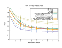
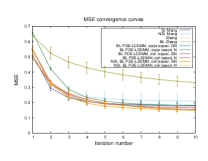
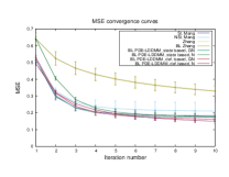
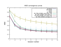
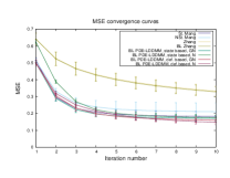
Figure 1: $MSE_{rel}$ convergence curves of the proposed methods for each BL domain size. For comparison purposes, the convergence curves of the benchmark methods in $\Omega$ are shown in all the plots.

Figure 1 shows the mean and standard deviation of the $MSE_{rel}$ convergence curves obtained during the optimization. The proposed methods with Gauss-Newton optimization showed a convergence pattern similar to stationary Mang. et al. method, with the exception of BL sizes equal to $16$ where the spatial methods showed a faster convergence. Second-order optimization methods outperformed gradient-descent as theoretically expected. Newton optimization in PDE-LDDMM based on the deformation state equation outperformed Gauss-Newton as theoretically expected. Surprisingly, Gauss-Newton showed a better convergence curve than Newton in PDE-LDDMM based on the state equation.

Benchmark methods, V-regularization, $\gamma=0$
Method Opt. $MSE_{rel}$ $\|g\|_{\infty,{rel}}$ $\max(J(\phi^{v}))$ $\min(J(\phi^{v}))$ PCG iter $time_{GPU}(s)$ St. Mang GN 18.29 $\pm$ 2.83 0.07 $\pm$ 0.05 3.70 $\pm$ 0.51 0.16 $\pm$ 0.05 43.73 $\pm$ 10.64 3104.41 $\pm$ 695.22 NSt. Mang GN 21.11 $\pm$ 5.18 0.20 $\pm$ 0.11 3.65 $\pm$ 0.85 0.15 $\pm$ 0.04 26.00 $\pm$ 15.21 5782.45 $\pm$ 1947.92 (*) Method Opt. $MSE_{rel}$ $\|g\|_{\infty,{rel}}$ $\max(J(\phi^{v}))$ $\min(J(\phi^{v}))$ $time_{GPU}(s)$ Zhang GD 20.48 $\pm$ 1.84 0.04 $\pm$ 0.09 2.52 $\pm$ 0.22 0.19 $\pm$ 0.03 97.40 $\pm$ 10.06 4683.22 $\pm$ 1857.32 BL Zhang, 64 GD 20.79 $\pm$ 2.03 0.01 $\pm$ 0.00 2.72 $\pm$ 0.31 0.18 $\pm$ 0.03 97.87 $\pm$ 5.73 1086.28 $\pm$ 44.60 BL Zhang, 56 GD 20.80 $\pm$ 2.04 0.01 $\pm$ 0.00 2.72 $\pm$ 0.30 0.18 $\pm$ 0.03 97.67 $\pm$ 6.28 747.20 $\pm$ 32.76 BL Zhang, 48 GD 20.87 $\pm$ 2.04 0.01 $\pm$ 0.00 2.74 $\pm$ 0.30 0.19 $\pm$ 0.03 98.00 $\pm$ 5.49 543.06 $\pm$ 28.55 BL Zhang, 40 GD 21.00 $\pm$ 2.01 0.01 $\pm$ 0.00 2.71 $\pm$ 0.27 0.19 $\pm$ 0.03 98.87 $\pm$ 4.12 535.07 $\pm$ 25.87 BL Zhang, 32 GD 21.33 $\pm$ 2.03 0.00 $\pm$ 0.00 2.64 $\pm$ 0.31 0.20 $\pm$ 0.03 98.60 $\pm$ 5.42 588.65 $\pm$ 24.56 BL Zhang, 16 GD 25.77 $\pm$ 2.60 0.00 $\pm$ 0.00 2.40 $\pm$ 0.28 0.23 $\pm$ 0.04 100.00 $\pm$ 0.00 604.43 $\pm$ 25.21
St. BL PDE-LDDMM, state equation, $V$-regularization, $\gamma=0$
BL size Opt. $MSE_{rel}$ $\|g\|_{\infty,{rel}}$ $\max(J(\phi^{v}))$ $\min(J(\phi^{v}))$ PCG iter $time_{GPU}$ (s) 64 GN 17.15 $\pm$ 1.58 0.02 $\pm$ 0.01 3.15 $\pm$ 0.37 0.12 $\pm$ 0.07 50.00 $\pm$ 0.00 423.73 $\pm$ 1.85 56 GN 17.24 $\pm$ 1.59 0.02 $\pm$ 0.01 3.16 $\pm$ 0.37 0.12 $\pm$ 0.07 49.53 $\pm$ 0.52 381.33 $\pm$ 2.92 48 GN 17.41 $\pm$ 1.60 0.02 $\pm$ 0.01 3.14 $\pm$ 0.36 0.11 $\pm$ 0.07 49.00 $\pm$ 0.00 372.71 $\pm$ 2.12 40 GN 17.77 $\pm$ 1.63 0.02 $\pm$ 0.01 3.16 $\pm$ 0.38 0.11 $\pm$ 0.07 47.93 $\pm$ 0.96 364.03 $\pm$ 4.41 32 GN 18.53 $\pm$ 1.71 0.02 $\pm$ 0.01 3.10 $\pm$ 0.35 0.11 $\pm$ 0.07 46.87 $\pm$ 0.35 358.78 $\pm$ 3.04 16 GN 24.38 $\pm$ 2.34 0.02 $\pm$ 0.01 3.32 $\pm$ 0.73 0.17 $\pm$ 0.06 43.20 $\pm$ 1.08 335.40 $\pm$ 9.95 BL size Opt. $MSE_{rel}$ $\|g\|_{\infty,{rel}}$ $\max(J(\phi^{v}))$ $\min(J(\phi^{v}))$ PCG iter $time_{GPU}$ (s) 64 N 17.53 $\pm$ 1.60 0.03 $\pm$ 0.01 3.08 $\pm$ 0.28 0.11 $\pm$ 0.06 49.53 $\pm$ 0.64 853.19 $\pm$ 27.83 56 N 17.62 $\pm$ 1.62 0.03 $\pm$ 0.01 3.06 $\pm$ 0.31 0.11 $\pm$ 0.06 48.73 $\pm$ 0.59 710.48 $\pm$ 5.52 48 N 17.80 $\pm$ 1.63 0.03 $\pm$ 0.01 3.08 $\pm$ 0.33 0.11 $\pm$ 0.06 48.13 $\pm$ 0.83 644.01 $\pm$ 18.06 40 N 18.16 $\pm$ 1.69 0.03 $\pm$ 0.01 3.13 $\pm$ 0.38 0.11 $\pm$ 0.07 47.00 $\pm$ 0.38 598.04 $\pm$ 27.39 32 N 18.94 $\pm$ 1.75 0.03 $\pm$ 0.01 3.11 $\pm$ 0.34 0.11 $\pm$ 0.07 46.07 $\pm$ 0.96 554.64 $\pm$ 7.10 16 N 24.95 $\pm$ 2.42 0.02 $\pm$ 0.01 3.31 $\pm$ 0.81 0.16 $\pm$ 0.06 41.73 $\pm$ 1.03 480.10 $\pm$ 8.11
St. BL PDE-LDDMM, deformation state equation, $V$-regularization, $\gamma=0$
BL size Opt. $MSE_{rel}$ $\|g\|_{\infty,{rel}}$ $\max(J(\phi^{v}))$ $\min(J(\phi^{v}))$ PCG iter $time_{GPU}$ (s) 64 GN 16.04 $\pm$ 1.53 0.04 $\pm$ 0.01 3.88 $\pm$ 0.42 0.11 $\pm$ 0.04 49.47 $\pm$ 1.46 586.51 $\pm$ 9.33 56 GN 16.09 $\pm$ 1.52 0.03 $\pm$ 0.01 3.86 $\pm$ 0.41 0.11 $\pm$ 0.04 49.53 $\pm$ 0.52 502.26 $\pm$ 10.10 48 GN 16.25 $\pm$ 1.55 0.03 $\pm$ 0.01 3.84 $\pm$ 0.41 0.12 $\pm$ 0.05 49.00 $\pm$ 0.00 439.04 $\pm$ 9.63 40 GN 16.57 $\pm$ 1.59 0.03 $\pm$ 0.01 3.78 $\pm$ 0.48 0.13 $\pm$ 0.05 48.00 $\pm$ 1.00 402.28 $\pm$ 8.00 32 GN 17.32 $\pm$ 1.68 0.03 $\pm$ 0.01 3.76 $\pm$ 0.49 0.13 $\pm$ 0.05 46.80 $\pm$ 0.56 386.06 $\pm$ 10.88 16 GN 23.34 $\pm$ 2.29 0.03 $\pm$ 0.01 3.30 $\pm$ 0.61 0.17 $\pm$ 0.05 42.07 $\pm$ 1.28 334.60 $\pm$ 10.85 BL size Opt. $MSE_{rel}$ $\|g\|_{\infty,{rel}}$ $\max(J(\phi^{v}))$ $\min(J(\phi^{v}))$ PCG iter $time_{GPU}$ (s) 64 N 14.75 $\pm$ 1.38 0.10 $\pm$ 0.03 4.89 $\pm$ 0.68 0.08 $\pm$ 0.04 49.53 $\pm$ 0.83 900.40 $\pm$ 12.62 56 N 14.83 $\pm$ 1.38 0.11 $\pm$ 0.03 4.95 $\pm$ 0.72 0.08 $\pm$ 0.04 49.53 $\pm$ 0.83 752.90 $\pm$ 12.64 48 N 15.02 $\pm$ 1.40 0.12 $\pm$ 0.03 5.06 $\pm$ 0.77 0.08 $\pm$ 0.04 49.93 $\pm$ 0.26 666.53 $\pm$ 9.22 40 N 15.38 $\pm$ 1.43 0.11 $\pm$ 0.03 5.01 $\pm$ 0.74 0.08 $\pm$ 0.04 50.00 $\pm$ 0.00 593.95 $\pm$ 7.08 32 N 16.19 $\pm$ 1.50 0.11 $\pm$ 0.03 4.92 $\pm$ 0.68 0.09 $\pm$ 0.04 50.00 $\pm$ 0.00 573.59 $\pm$ 8.87 16 N 22.69 $\pm$ 2.26 0.08 $\pm$ 0.03 4.21 $\pm$ 0.77 0.11 $\pm$ 0.03 50.00 $\pm$ 0.00 514.33 $\pm$ 6.23
NSt. BL PDE-LDDMM, deformation state equation, V-regularization, $\gamma=0$
BL size Opt. $MSE_{rel}$ $\|g\|_{\infty,{rel}}$ $\max(J(\phi^{v}))$ $\min(J(\phi^{v}))$ PCG iter $time_{GPU}$ (s) 40 GN 14.93 $\pm$ 1.40 0.04 $\pm$ 0.01 4.87 $\pm$ 0.77 0.08 $\pm$ 0.04 48.40 $\pm$ 0.83 6427.13 $\pm$ 346.89 32 GN 15.72 $\pm$ 1.52 0.04 $\pm$ 0.01 4.74 $\pm$ 0.77 0.09 $\pm$ 0.04 46.87 $\pm$ 0.35 5729.49 $\pm$ 306.90 16 GN 21.94 $\pm$ 2.12 0.04 $\pm$ 0.01 3.96 $\pm$ 0.89 0.13 $\pm$ 0.04 42.47 $\pm$ 1.46 4729.42 $\pm$ 201.01 40 N 14.83 $\pm$ 1.33 0.11 $\pm$ 0.04 6.91 $\pm$ 2.16 0.05 $\pm$ 0.03 49.80 $\pm$ 0.41 8098.13 $\pm$ 308.54 32 N 15.59 $\pm$ 1.39 0.11 $\pm$ 0.03 6.23 $\pm$ 1.32 0.05 $\pm$ 0.03 50.00 $\pm$ 0.00 8609.06 $\pm$ 384.97 16 N 22.19 $\pm$ 2.23 0.09 $\pm$ 0.03 4.89 $\pm$ 1.06 0.08 $\pm$ 0.03 49.60 $\pm$ 1.12 7167.19 $\pm$ 330.20

Table 1: Quantitative results relevant for the evaluation of the benchmark and the proposed methods. In Opt. column, GD stands for gradient-descent optimization, and N and GN stand for Newton- and Gauss-Newton- Krylov optimization, respectively. (*) Recall that the implementation of NSt. Mang method was performed partially in the CPU.

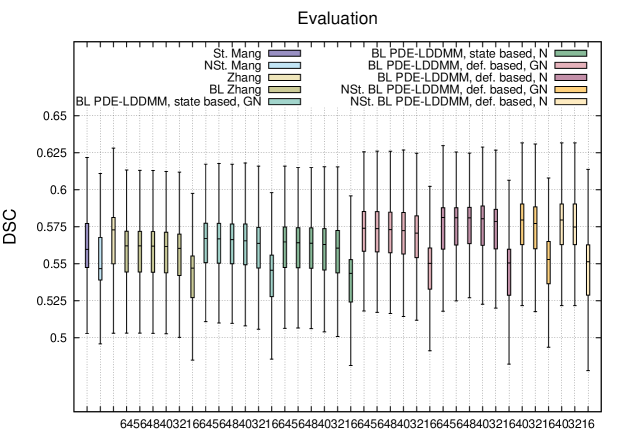
Figure 2: Up, VRAM peak memory (MBs) reached through the experiments by the registration methods. Down, volume overlap obtained by the registration methods measured in terms of the DSC between the warped and the corresponding manual target segmentation. Box and whisker plots show the distribution of the DSC averaged over the 32 NIREP manual segmentations. The tick labels show the size of the band-limited space when applicable.

4.2 Qualitative results

For a qualitative assessment of the registration methods, we show the registration results obtained by the considered methods in a selected experiment representative of a difficult deformable registration problem. For the methods parameterized in the space of band-limited vector fields, we selected a BL size of $32\times 32\times 32$. The methods parameterized in this space show a good compromise between efficiency and accuracy. Figure 3 shows the warped images and the difference between the warped and the target image after registration.

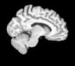
source	target

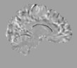
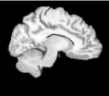
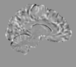
St. Mang		NSt. Mang
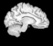
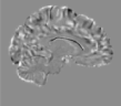
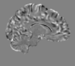
Zhang		BL Zhang
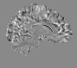
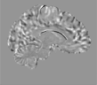
St. BL PDE-LDDMM state equation, GN		St. BL PDE-LDDMM state equation, N
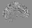
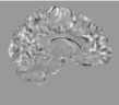
St. BL PDE-LDDMM def. equation, GN		St. BL PDE-LDDMM def. equation, N
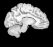
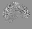
NSt. BL PDE-LDDMM def. equation, GN		NSt. BL PDE-LDDMM def. equation, N

Figure 3: Sagittal view of the warped sources and the intensity differences after registration for the methods considered in the comparison. $V$-regularization, $\gamma=0$, BL size of $32\times 32\times 32$.

4.3 Evaluation

The evaluation of the methods is based on the accuracy of the registration results for template-based segmentation. This is a widely extended criterion for non-rigid registration evaluation [33, 34]. We use the manual segmentations provided with the NIREP database as the gold standard. The Dice Similarity Coefficient (DSC) is selected as the evaluation metric. Figure 2 shows in the shape of box-and-whisker plots the statistical distribution of the DSC values obtained after the registration across the 32 segmented structures. The best performing method was our proposed BL PDE-LDDMM based on the deformation state equation. The performance of BL PDE-LDDMM based on the state equation was slightly lower and similar to the performance achieved by St. Mang method. Gauss-Newton achieved results similar to Newton optimization. For BL sizes ranging from 64 to 32, all methods performed similarly. The performance for BL size of 16 was degraded, indicating that the limit in acceptable BL size selection is above this value.

4.4 Quantitative results for incompressible $H^{1}$ regularization

Finally, Table 2 shows the quantitative results of interest for the proposed methods with Gauss-Newton and incompressible $H^{1}$-regularization. The model of deformation in inter-subject brain image registration is not compressible. Therefore, these experiments should be analyzed as a proof of concept regarding the ability of our methods to compute incompressible velocity fields. In this case, PDE-LDDMM based on the state equation slightly outperformed PDE-LDDMM on the deformation state equation. All the Jacobian determinants remained equal to 1. This shows the ability of our proposed methods to respect the incompressibility constraint.

BL PDE-LDDMM, state equation, $H^{1}$-regularization, $\gamma=1$

BL size	Opt.	$MSE_{rel}$	$\|g\|_{\infty,{rel}}$	$\max(J(\phi^{v}))$	$\min(J(\phi^{v}))$	PCG iter	$time_{GPU}$ (s)
$64$	GN	12.95 $\pm$ 1.36	0.07 $\pm$ 0.04	1.00 $\pm$ 0.00	1.00 $\pm$ 0.00	34.00 $\pm$ 1.41	*422.14 $\pm$ **6.12
$56$	GN	13.59 $\pm$ 1.50	0.08 $\pm$ 0.03	1.00 $\pm$ 0.00	1.00 $\pm$ 0.00	32.73 $\pm$ 1.98	*392.58 $\pm$ **0.82
$48$	GN	14.43 $\pm$ 1.46	0.08 $\pm$ 0.03	1.00 $\pm$ 0.00	1.00 $\pm$ 0.00	31.66 $\pm$ 1.71	*383.49 $\pm$ **4.41
$40$	GN	15.54 $\pm$ 1.70	0.07 $\pm$ 0.02	1.00 $\pm$ 0.00	1.00 $\pm$ 0.00	31.13 $\pm$ 2.06	*388.12 $\pm$ *12.29
$32$	GN	17.44 $\pm$ 1.77	0.07 $\pm$ 0.03	1.00 $\pm$ 0.00	1.00 $\pm$ 0.00	30.79 $\pm$ 2.00	*384.43 $\pm$ **3.20
$16$	GN	27.39 $\pm$ 2.41	0.05 $\pm$ 0.02	1.00 $\pm$ 0.00	1.00 $\pm$ 0.00	32.00 $\pm$ 1.06	*362.62 $\pm$ **4.49

BL PDE-LDDMM, deformation state equation, $H^{1}$-regularization, $\gamma=1$

BL size	Opt.	$MSE_{rel}$	$\|g\|_{\infty,{rel}}$	$\max(J(\phi^{v}))$	$\min(J(\phi^{v}))$	PCG iter	$time_{GPU}$ (s)
$64$	GN	13.89 $\pm$ 2.01	0.10 $\pm$ 0.04	1.00 $\pm$ 0.00	1.00 $\pm$ 0.00	38.86 $\pm$ 1.68	*731.81 $\pm$ *15.82
$56$	GN	14.43 $\pm$ 2.21	0.11 $\pm$ 5.30	1.00 $\pm$ 0.00	1.00 $\pm$ 0.00	38.00 $\pm$ 2.50	*535.94 $\pm$ *18.96
$48$	GN	15.16 $\pm$ 2.20	0.11 $\pm$ 0.04	1.00 $\pm$ 0.00	1.00 $\pm$ 0.00	37.13 $\pm$ 2.06	*479.10 $\pm$ *14.55
$40$	GN	16.38 $\pm$ 2.34	0.11 $\pm$ 0.05	1.00 $\pm$ 0.00	1.00 $\pm$ 0.00	35.93 $\pm$ 2.12	*439.13 $\pm$ **2.07
$32$	GN	18.25 $\pm$ 2.70	0.11 $\pm$ 0.07	1.00 $\pm$ 0.00	1.00 $\pm$ 0.00	34.73 $\pm$ 3.36	*407.88 $\pm$ **6.69
$16$	GN	27.89 $\pm$ 2.95	0.09 $\pm$ 0.04	1.00 $\pm$ 0.00	1.00 $\pm$ 0.00	37.00 $\pm$ 1.51	*356.92 $\pm$ **3.96

Table 2: Quantitative results of interest for the evaluation of the proposed method. Results obtained with incompressible $H^{1}$-regularization and Gauss-Newton-Krylov optimization.

5 Conclusions

In this work, we have proposed two PDE-constrained LDDMM methods parameterized in the space of band-limited vector fields and optimized with Newton- and Gauss-Newton- Krylov methods. The proposed methods depart from two versions of PDE-constrained LDDMM that were optimized using gradient information. We have derived the expressions of the Hessian-vector products and we have computed the gradient and the Hessian-vector products in the space of band-limited vector fields. The performance of the proposed methods has been evaluated with respect to the state of the art methods most related to our work.

The PDE-constrained LDDMM methods were selected among those that allowed working directly with velocity and deformation fields. This circumvented solving the state and adjoint equations in the space of band-limited images, which may be subtle for small BL sizes. It should be noticed that some computations of PDE-LDDMM based on the state equation need to be performed in the spatial domain, while PDE-LDDMM based on the deformation state equation is fully posed in the space of band-limited vector fields.

The proposed methods have shown a competitive performance with respect to the benchmark methods. From them, PDE-LDDMM based on the deformation state equation has shown to outperform the others. The use of Gauss-Newton optimization and a BL size equal to 32 has shown to be a good configuration for obtaining acceptable registration results in an efficient way, while Newton optimization slightly outperformed these results with a considerable increase of the computational time. Indeed, our methods can preserve the incompressibility constraint.

The results obtained in this work reinforce Zhang et al.’s idea on the usefulness of working in the space of band-limited vector fields for LDDMM applications, even in the delicate framework of PDE-constrained LDDMM. In future work, we will analyze the applicability of the proposed methods in Computational Anatomy applications and we will extend the PDE-LDDMM formulation to more complex physical models.

References

- [1] Ruhnau, P., Schnorr, C.: Optical stokes flow estimation: an imaging-based control approach. Exp. Fluids 42 (2007) 61 – 78
- [2] Ruhnau, P., Stahl, A., Schnorr, C.: Variational estimation of experimental fluid flows with physics-based spatio-temporal regularization. Meas. Sc. and Techn. 18(3) (2007)
- [3] Papadakis, N., Corpetti, T., Memin, E.: Dynamically consistent optical flow estimation. Proc. of the 11th IEEE International Conference on Computer Vision (ICCV’07) (2007)
- [4] Papadakis, N., , Memin, E.: Variational assimilation of fluid motion from image sequence. SIAM J. Imaging Sciences 1(4) (2008) 343 – 363
- [5] Alvarez, L., Castano, C.A., Garcia, M., Krissian, K., Mazorra, L., Salgado, A., Sanchez, J.: A new energy-based method for 3D motion estimation of incompressible PIV flows. Comput. Vis. Image Und. 113 (2009) 802 – 810
- [6] Cuzon, A., Memin, E.: A stochastic filtering technique for fluid flow velocity fields tracking. IEEE Trans. Pattern Anal. Mach. Intell. 31(7) (2009) 1278 – 1293
- [7] Heitz, D., Memin, E., Schnorr, C.: Variational fluid flow measurements from image sequences: synopsis and perspectives. Exp. Fluids 48 (2010) 369 – 393
- [8] Herlin, I., Bereziat, D., Mercier, N., Zhuk, S.: Divergence free motion estimation. Proc. of the 12th European Conference on Computer Vision (ECCV’12), Lecture Notes in Computer Science (2012) 15 – 27
- [9] Heas, P., Herzet, C., Memin, E., Heitz, D., Mininni, P.D.: Bayesian estimation of turbulent motion. IEEE Trans. Pattern Anal. Mach. Intell. 35(6) (2013) 1343 – 1356
- [10] Zhong, Q., Yang, H., Yin, Z.: An optical flow algorithm based on gradient constancy assumption for PIV image processing. Meas. Sc. and Techn. 28(5) (2017)
- [11] Bistoquet, A., Oshinski, J., Skrinjar, O.: Myocardial deformation recovery from cine mri using a nearly incompressible biventricular model. Med. Image Anal. 12 (2008) 69 – 85
- [12] Mansi, T., Pennec, X., Sermesant, M., Delingette, H., Ayache, N.: iLogDemons: A demons-based registration algorithm for tracking incompressible elastic biological tissues. Int. J. Comput. Vision 92(1) (2011) 92 – 111
- [13] Risser, L., Vialard, F.X., Baluwala, H.Y., Schnabel, J.A.: Piecewise-diffeomorphic image registration: Application to the motion correction of 3D CT lung images using sliding conditions. Med. Image Anal. 17(2) (2012) 182 – 193
- [14] Baluwala, H.Y., Risser, L., Schnabel, J.A., Saddi, K.A.: Toward physiologically motivated registration of diagnostic CT and PET/CT of lung volumes. Med. Phys. 40 (2013)
- [15] Papiez, B.W., Heinrich, M.P., Fehrenbach, J., Risser, L., Schnabel, J.A.: An implicit sliding-motion preserving regularization via bilateral filtering for deformable image registration. Med. Image Anal. 18 (2014) 1299 – 1311
- [16] Hogea, C., Davatzikos, C., Biros, G.: Brain-tumor interaction biophysical models for medical image registration. SIAM J. Imaging Sciences 30 (2008) 3050 – 3072
- [17] Mang, A., Toma, A., Schuetz, T.A., Becker, S., Eckey, T., Mohr, C., Petersen, D., Buzug, T.M.: Biophysical modeling of brain tumor progression: From unconditionally stable explicit time integration to an inverse problem with parabolic PDE constraints for model calibration. Med. Phys. 39(7) (2012) 4444–4460
- [18] Sotiras, A., Davatzikos, C., Paragios, N.: Deformable medical image registration: A survey. IEEE Trans. Med. Imaging 32(7) (2013) 1153 – 1190
- [19] Miller, M.I.: Computational anatomy: shape, growth, and atrophy comparison via diffeomorphisms. Neuroimage 23 (2004) 19–33
- [20] Hart, G.L., Zach, C., Niethammer, M.: An optimal control approach for deformable registration. Proc. of the IEEE Conference on Computer Vision and Pattern Recognition (CVPR’09) (2009)
- [21] Vialard, F.X., Risser, L., Rueckert, D., Cotter, C.J.: Diffeomorphic 3D image registration via geodesic shooting using an efficient adjoint calculation. Int. J. Comput. Vision 97(2) (2011) 229 – 241
- [22] Mang, A., Biros, G.: An inexact Newton-Krylov algorithm for constrained diffeomorphic image registration. SIAM J. Imaging Sciences 8(2) (2015) 1030–1069
- [23] Mang, A., Biros, G.: Constrained H1 regularization schemes for diffeomorphic image registration. SIAM J. Imaging Sciences (2016)
- [24] Mang, A., Ruthotto, L.: A lagrangian Gauss–Newton–Krylov solver for mass- and intensity-preserving diffeomorphic image registration. SIAM J. Sci. Comput. 39(5) (2017) B860 – B885
- [25] Mang, A., Biros, G.: A semi-lagrangian two-level preconditioned Newton-Krylov solver for constrained diffeomorphic image registration. SIAM J. Sci. Comput. 39(6) (2017) B1064 – B1101
- [26] Mang, A., Gholami, A., Biros, G.: Distributed-memory large-deformation diffeomorphic 3D image registration. Proc. of ACM/IEEE SuperComputing conference (SC16) (2016)
- [27] Zhang, M., Fletcher, P.T.: Finite-dimensional Lie algebras for fast diffeomorphic image registration. Proc. of International Conference on Information Processing and Medical Imaging (IPMI’15), Lecture Notes in Computer Science (2015)
- [28] Zhang, M., Liao, R., Dalca, A.V., Truk, E.A., Luo, J., Grant, P.E., Golland, P.: Frequency diffeomorphisms for efficient image registration. Proc. of International Conference on Information Processing and Medical Imaging (IPMI’17), Lecture Notes in Computer Science (2017) 559–570
- [29] Younes, L.: Jacobi fields in groups of diffeomorphisms and applications. Q. Appl. Math. 65 (2007) 113 – 134
- [30] Polzin, T., Niethammer, M., Heinrich, M.P., Handels, H., Modersitzki, J.: Memory efficient LDDMM for lung CT. (2014) 28–36
- [31] Song, J.H., Christensen, G.E., Hawley, J.A., Wei, Y., Kuhl, J.G.: Evaluating image rgistration using NIREP. WBIR 2010, LNCS 6204 (2010) 140 – 150
- [32] Beg, M.F., Miller, M.I., Trouve, A., Younes, L.: Computing large deformation metric mappings via geodesic flows of diffeomorphisms. Int. J. Comput. Vision 61 (2) (2005) 139–157
- [33] Klein, A., et al.: Evaluation of 14 nonlinear deformation algorithms applied to human brain MRI registration. Neuroimage 46(3) (2009) 786–802
- [34] Ou, Y., Akbari, H., Bilello, M., Da, X., Davatzikos, C.: Comparative evaluation of registration algorithms in different brain databases with varying difficulty: results and insights. IEEE Trans. Med. Imaging 33(10) (2014) 2039 – 2065