Quantum Pontryagin Principle under Continuous Measurements

Abstract

In this paper we develop the theory of the quantum Pontryagin principle for continuous measurements and feedback. The analysis is carried out under the assumption of compatible events in the output channel. The plant is a quantum system, which generally is in a mixed state, coupled to a continuous measurement channel. The Pontryagin Maximum Principle is derived in both the Schrödinger picture and Heisenberg picture, in particular in statistical moment coordinates. To avoid solving stochastic equations we derive a LQG scheme which is more suitable for control purposes. Finally, we use the quantum harmonic oscillator as a concrete example to illustrate the performance of the controller.

I Introduction

Quantum optimal control (QOC, for short) is a powerful tool for achieving quantum control objectives in many practical problems of interest for the emerging field of Quantum Technologies ( see wiseman2010quantum ; Glaser2015 and the references therein). It has been successfully used in a vast area of quantum applications from physical chemistry Shapiro2012 , to multi-dimensional nuclear magnetic resonance experiments Khaneja2003311 , through time-optimal control problems PhysRevA.92.063415 ; PhysRevB.93.035423 .

In constrained optimization, the Pontryagin Maximum Principle (PMP) is an attractive technique based on the variational method of Lagrange multipliers. Few results have appeared in recent years based on the explicit calculation of the extremal solutions and those are applicable only to discrete low-dimensional systems: fast generation of a given-structure wave package Glovinskii ; adiabatic population transfer in $\Lambda$-systems via intermediate states that are subject to decay PhysRevA.85.033417 ; fast adiabatic cooling in harmonic traps and non-interacting collection of harmonic oscillators with a shared frequency 0295-5075-96-6-60015 ; B816102J ; stefanatos11 ; stefanatos17 ; stefanatos17b optimal cooling power of a reciprocating quantum refrigerator; 0295-5075-85-3-30008 time-optimal control for one or two spins (or qubits) PhysRevA.74.022306 ; PhysRevA.88.062326 ; PhysRevLett.104.083001 ; PhysRevA.63.032308 ; PhysRevA.88.043422 ; dalesandro01 ; boscain02 ; boscain06 ; stefanatos10 ; bonnard09 ; minimum-time adiabatic-like paths for the expansion of a quantum piston Stefanatos20133079 . In those applications the external controls were determined via a deterministic Pontryagin principle based on the controlled Schrödinger equation:

$$\frac{d}{dt}\,\left|\psi\right\rangle=-\frac{i}{\hbar}\,H\left(u\right)\left|\psi\right\rangle$$

where $H\left(u\right)$ is the Hamiltonian driven by a control action $u$ and $\left|\psi\right\rangle$ is a state vector in the Hilbert space of the system to be controlled. In most of these aforementioned approaches, the feedback is absent roloff09 . In other words, the system is not subjected to any measurement and a subsequent quantum filtering, which reduces the Pontryagin principle to its deterministic version (see sugny08 ; wang11 ; egger14 for examples and applications of quantum optimal control with measurements). On the other hand, a few results promote ad-hoc model-dependent solutionsGlovinskii .

Motivated by these previous studies, here we address the task of stating both a firm theoretical ground and a formalization of the quantum PMP for systems with quantum feedback provided by continuous weak measurements Jacobs06 ; Clerk10 . This may help the subsequent verification procedures to check if the resulting control is optimal Jacobs08 . In addition, a quantum Pontryagin principle would allow to tackle with state constraints.

In the Schrödinger picture the conditional dynamics of the system evolving under these weak measurements is described by quantum filtering theory. Filtering concerns the processing of the information yielded by the measurement process. This information is generally incomplete because the state is not fully accessible by the measurement setting, and is inherently corrupted by noise. In this context, optimal control problems are solved by using a cost function expressed in terms of the state given by the filter, which is often called an information state. The quantum Belavkin filter, or stochastic master equation, computes this information state belavkin99 .

This work is organized as follows. In Section II the continuous measurement of a quantum system and the subsequent filtering of the outcomes of this measurement is analyzed in terms of a quantum probability space. There, measurement operators are considered for the abelian subalgebra generated by commuting projectors. As a result, filtrations in the quantum probability space as well as adapted processes are defined in terms of von Neumann subalgebras. This allows us to define feasible and admissible control actions in terms of operators. Section III is devoted to the derivation of the quantum PMP in a global form from the Hamilton-Jacobi-Bellman equation in the Schrödinger picture. The result is a system of coupled forward-backward stochastic differential equations that replaces the HJB partial differential equation.

In addition, as a very natural way of defining state-space realizations is in the Heisenberg picture, particularly in coordinates of expectation and variance, we derive in IV a Hamilton-Jacobi-Bellman equation in these coordinates as a preceding step to build a quantum PMP. One drawback of stochastic PMP is that the control problem cannot be solved in closed form, and one needs to resort to numerical optimization. To overcome this difficulty, for quantum linear models petersen16 we derive a LQG from the quantum PMP based on the statistical moment coordinates. This adds a novel result to the significant literature on measurement based optimal control of quantum linear systems (see dong09 ; nori17 and references therein). In Section V we illustrate the application of the quantum PMP to a dissipative quantum harmonic oscillator. Finally, the concluding remarks are given in Section VI.

II Quantum Optimal Control Problem

As we formulate the quantum Pontryagin’s Principle under continuous measurements, first we review how the quantum measurement and filtering problem can be rephrased in terms of the optimal estimation of the output of a noisy quantum channel.

With every quantum system there is a separable complex Hilbert space $\mathcal{H}$ on which a von Neumann algebra of linear operators $\mathcal{A}$ is defined (a Banach algebra of bounded operators on $\mathcal{H}$). In general, one also needs the predual space $\mathcal{A}_{\star}$ and particularly those positive elements of $\mathcal{A}_{\star}$ which are unitary normed, called density operators $\rho$ or normal states. A quantum probability space can be defined as the pair $\left(\mathcal{A},\rho\right)$.

In this paper, quantum feedback is generated through a continuous quantum measurement on a quantum system. Following belavkin99 , this continuous measurement is implemented by an indirect measurement of the operators corresponding to a semi-classical field coupled to the system. After measurement, the change of the density operator of the system $\rho$ is described through an optimal estimator based on the results of measurements in this field. The state of the field lies in the Hilbert space $\mathcal{F}$ and initially is in its vacuum state $\phi$. We observe compatible events on this measurement channel through projectors $\{P_{\omega}\}_{\omega\in\Omega}$ that generate an abelian subalgebra $\mathcal{B}\subset\mathcal{B}(\mathcal{F})$ where $\Omega$ is the space of measurement results (eigenvalues) for these commuting operators. In this sense, all the field operators $W\in\mathcal{B}$ which are linear combinations of the commuting projectors are in one-to-one correspondence with classical random variables as functions from the data space $\Omega$ into $\mathbb{R}$. The interaction between the quantum system and the field is described in terms of a unitary operator $U$ such that,

$$\rho\otimes\phi\to U(t)(\rho\otimes\phi)U^{\dagger}(t)\,.$$

With this, the conditional evolution after a measurement on the quantum system is given by

$$\rho(t)\to\rho_{\omega}(t)\>=\frac{\textrm{Tr}_{\mathcal{F}}[U(t)(\rho\otimes\phi)U^{\dagger}(t)(I\otimes P_{\omega})]}{\textrm{Tr}[U(t)(\rho\otimes\phi)U^{\dagger}(t)(I\otimes P_{\omega})]}$$ (1)

which gives the posterior state $\rho_{\omega}(t)$ that implements the Bayes law of conditioning for the measurement result $\omega\in\Omega$, normalized with respect to the output probabilities $\mathbb{P}(\omega)=\textrm{Tr}[U(t)(\rho\otimes\phi)U^{\dagger}(t)(I\otimes P_{\omega})]$ and $\textrm{Tr}_{\mathcal{F}}$ denotes the partial trace over $\mathcal{F}$.

The posterior state must be considered as a classical random variable $\rho_{\bullet}:\Omega\to\mathcal{A}_{\star}$ taking values $\rho_{\omega}$ in the space $\mathcal{A}_{\star}$ of states on $\mathcal{A}$. It gives the conditional expectation

$$\mathbb{E}[X^{\prime}|Y]=\langle\rho_{\bullet},X\rangle$$

which amounts to the least squares estimator of the system operator $X^{\prime}_{t}=U^{\dagger}(t)(X\otimes I)U(t)$ after interaction, with respect to the output operators $Y_{t}:=U^{\dagger}(t)(I\otimes W)U(t)$.

Within this framework, the dynamical coupling between the system and the field acts as a quantum noise bath on the system. The bath is then modelled by a Fock space $\mathcal{F}$ and $\mathcal{W}:=\mathcal{B}(\mathcal{F})$ is the algebra of bounded operators on $\mathcal{F}$. Thus, the continuous measurement of our system is understood as measurements of a Wiener process in the field described by field quadrature operators $W_{t}=A_{t}+A_{t}^{\dagger}$ where $A_{t}\in\mathcal{W}$ is the annihilation operator on $\mathcal{F}$. Quantum stochastic calculus can be defined using the annihilation process and its adjoint, the creation process $A^{\dagger}_{t}$ as the fundamental diffusive adapted processes whose increments $dA_{t}$, $dA^{\dagger}_{t}$ are considered as operators acting in the Fock space by using the multiplication table DBLP:journals/siamco/BoutenHJ07 ; parthasarathy2012introduction

$$\begin{array}[]{l}(dt)^{2}=0,\quad dtdA_{t}=0=dtdA^{\dagger}_{t},\\ dA_{t}^{\dagger}dA_{t}=0,\quad dA_{t}dA_{t}^{\dagger}=dt.\end{array}$$ (2)

Denoting $L$ as the operator that models the coupling of the system to the measurement channel, a time continuous measurement of $W_{t}$ in the output channel represents an indirect measurement of $L_{t}+L_{t}^{\dagger}\in\mathcal{A}_{t}$ as can be seen from the quantum Itô formula applied to the directly observable output operators $Y_{t}=U(t)^{\dagger}(I\otimes W_{t})U(t)$:

$$dY_{t}=(L_{t}+L^{\dagger}_{t})\otimes dt+I\otimes dW_{t}\,.$$ (3)

In order to estimate the value of dynamical variables for which only an incomplete knowledge is provided through the indirect kind of oservations described above, some filtering equations are needed. Belavkin was the first to provide the quantum filtering equation which describes the optimal estimate of a density matrix conditioned by the classical output of a noisy quantum channel. The conditional expectation $\mathbb{E}[X_{t}|Y_{t}]$ gives the least squares estimator $\hat{X}_{t}$ of a conditional operator $X_{t}\in\mathcal{A}_{t}$ on the output operators $Y_{t}$. This is equivalent to a classical random variable on the space of measurement trajectories $\Omega_{T}:=\{\omega_{\tau}|0\leq t\leq T$ s.t. $\omega_{t}$ is an eigenvalue of $Y_{t}\}$ with $T\in\left(0,\infty\right)$ fixed. This conditional expectation is most conveniently written in the Schrödinger picture $\mathbb{E}[X_{t}|Y_{t}]=\langle\rho_{\bullet}(t),X\rangle$ for the solution $\rho_{\bullet}(t)$ to the stochastic nonlinear Schrödinger-like differential equation

$$d\rho_{\bullet}\left(t\right)=w\left(t,\rho_{\bullet}\left(t\right)\right)dt+\sigma\left(\rho_{\bullet}\left(t\right)\right)dW_{t}$$ (4)

called the Belavkin quantum filter in which Ito calculus $dW_{t}\,dW_{t}=dt$ holds. In Eq.$(\ref{EQ1})$ $w:\left[0,T\right]\times\mathcal{S}\rightarrow\mathcal{S}$, with $\mathcal{S}\subset\mathcal{A}_{\star}$ the convex set of density operators, refers to the unconditional evolution of states given by the dual of a Lindblad generator $\mathcal{L}$:

$$w\left(t,\rho_{\bullet}(t)\right)=\mathcal{L}^{\dagger}\left(\rho_{\bullet}(t)\right)=-\frac{i}{\hbar}\left[H,\rho_{\bullet}(t)\right]+\frac{1}{2}\left(L\left[\rho_{\bullet}(t),L^{\dagger}\right]+\left[L,\rho_{\bullet}(t)\right]L^{\dagger}\right)\,,$$

and the fluctuation operator $\sigma:\mathcal{S}\rightarrow\mathcal{S}$ is given by,

$$\sigma(\rho_{\bullet}(t))=\rho_{\bullet}(t)L^{\dagger}+L\rho_{\bullet}(t)-\langle\rho_{\bullet}(t),L^{\dagger}+L\rangle\rho_{\bullet}(t)\,.$$

Equation (4) defines a filtered quantum probability space $\left\{\left(\mathcal{A},\rho,\mathcal{A}_{t]}\right),t\geq 0\right\}$ satisfying the usual condition ( i.e. $\left(\mathcal{A},\rho\right)$ is complete, $\mathbf{I}\in\mathcal{A}_{0]}$ and $\left\{\mathcal{A}_{t]},t\geq 0\right\}$ is right continuous).

By the information field $\left\{\mathcal{A}_{t]},t\geq 0\right\}$, the controller is well-informed of what has happened in the past but, because of the uncertainty of the system, it is not able to predict the future. As a consequence there exists a non-anticipative restriction on the controller: for any instant the controller cannot decide its control action before the instant occurs. This restriction is expressed in mathematical terms as "$u\left(\cdot\right)$ is $\left\{\mathcal{A}_{t]}\right\}_{t>0}$ adapted", and the control is taken from the set

$$\mathcal{U}_{\left[0,T\right]}=\left\{u:\Omega_{T}\times\left[0,T\right]\rightarrow U:u\left(\cdot\right)\text{ is }\left\{\mathcal{A}_{t]}\right\}_{t>0}\text{ adapted}\right\}$$

Any $u_{\bullet}\left(\cdot\right)\in\mathcal{U}_{\left[0,T\right]}$ is called a feasible control. In particular fixing a control the drift and the dispersion depend on $\Omega_{T}$, i.e. $w,\sigma:\Omega_{T}\times\mathbb{R}^{+}\rightarrow\mathcal{A}_{\star}$. Given a $\mathcal{A}_{0]}$-measurable density matrix $\rho$ for every $u_{\bullet}\left(\cdot\right)$ the master equation 4 admits a strong solution $\rho\left(t;u\right)$ ( seen as a continuous $\left\{\mathcal{A}_{t]},t\geq 0\right\}-$adapted process) if

(i) $\rho\left(0\right)$ is almost sure in probability.

(ii) $\int_{0}^{t}\left(\left\|w\left(\tau,\rho_{\omega}\left(\tau\right),u_{\omega}\left(\tau\right)\right)\right\|+\left\|\sigma\left(\tau,\rho_{\omega}\left(\tau\right)\right)\right\|^{2}\right)d\tau<\infty$ for $t\geq 0$, almost sure in probability for $\omega\in\Omega_{T}$.

(iii) $\rho\left(t\right)=\rho+\int_{0}^{t}w\left(\tau,\rho,u\right)d\tau+\int_{0}^{t}\sigma\left(\tau,\rho\right)dW\left(\tau\right)$, $t\geq 0$, almost sure in probability
The adapted solution exists and it is unique if the drift and the dispersion are continuous measurable functions and they satisfy a Lipschitz condition with respect to $\rho$.

The adapted solution exists and it is unique if the drift and the dispersion are continuous measurable functions and they satisfy a Lipschitz condition with respect to $\rho$.

Let $\rho_{\bullet}\left(\cdot\right)$ be the solution to the filtering equation with initial condition $\rho_{\bullet}\left(0\right)=\rho$. The cost J for a feasible control action $u_{\bullet}\left(\cdot\right)$ is a random variable on $\Omega_{T}$, i.e. $\emph{J}:\Omega_{T}\times\mathcal{U}_{\left[0,T\right]}\times\mathcal{S}\times\left[0,T\right]\rightarrow\mathbb{R}$, defined by

$$\emph{J}_{\bullet}\left(u_{\bullet}\left(\cdot\right);\rho_{\bullet}\left(\cdot\right),t\right)=\int_{0}^{T}\emph{C}\left(\tau,u_{\bullet}\left(\tau\right),\rho_{\bullet}\left(\tau\right)\right)d\tau+\emph{M}\left(\rho_{\bullet}\left(T\right)\right)$$ (5)

where the cost density C and the terminal cost M are linear; for each $\omega\in\Omega_{T}$ and each instant $\tau\in\left(0,T\right]$:

$$\emph{C}\left(u_{\omega}\left(\tau\right),\rho_{\omega}\left(\tau\right)\right) = \left\langle\rho_{\omega}\left(\tau\right),C\left(\tau,u_{\omega}\left(\tau\right)\right)\right\rangle$$

$$\emph{M}\left(\rho_{\omega}\left(T\right)\right) = \left\langle\rho_{\omega},M\right\rangle$$

with $C$ and $M$ positive self-adjoint operators. Note that this cost may be different according to the requirements of the QOC problem, such as minimizing the control time, the control energy, the error between the final state and target state, or a combination of these. The goal is to minimize the criterion by selecting a nonanticipative decision among the ones satisfying all the quantum state constraints:

Definition 1.

Let $\left\{\left(\mathcal{A},\rho,\mathcal{A}_{t]}\right),t\geq 0\right\}$ be a filtered quantum probability space with the usual condition and let $W$ be a given standard $\left\{\mathcal{A}_{t]},t\geq 0\right\}-$Wiener process. A control $u_{\bullet}\left(\cdot\right)$ is called q-admissible, and $\left(\rho_{\bullet}\left(\cdot\right),u_{\bullet}\left(\cdot\right)\right)$ is a q-admissible pair if
(i) $u_{\bullet}\left(\cdot\right)\in\mathcal{U}_{\left[0,T\right]}$.
(ii) $\rho_{\bullet}\left(\cdot\right)$ is the unique solution to the master equation $\left(\ref{EQ1}\right)$.
(iii) $\rho_{\bullet}\left(\cdot\right)$ satisfies a prescribed state constraint.
(iv) For each $\omega\in\Omega_{T}$, $\emph{C}\left(\cdot,u_{\omega}\left(\tau\right),\rho_{\omega}\left(\tau\right)\right)\in L_{\mathcal{A}}^{1}\left(0,T;\mathbb{R}\right)$, $\emph{S}\left(\rho_{\omega}\left(T\right)\right)\in L_{\mathcal{A}_{T}}^{1}\left(\Omega_{T};\mathbb{R}\right)$.

Here the spaces $L_{\mathcal{A}}^{1}\left(0,T;\mathbb{R}\right)$ and $L_{\mathcal{A}_{T}}^{1}\left(\Omega_{T};\mathbb{R}\right)$ are defined on the filtered probability space $\left\{\left(\mathcal{A},\rho,\mathcal{A}_{t]}\right),t\geq 0\right\}$: $L_{\mathcal{A}}^{1}\left(0,T;\mathbb{R}\right)$ is the set of all $\left\{\mathcal{A}_{\left.t\right]}\right\}_{t\geq 0}$-adapted $\mathbb{R}$-valued processes $X\left(\bullet\right)$ such that $\mathbb{E}\left[\int_{0}^{T}\left|X\left(t\right)\right|dt\right]<\infty$ and $L_{\mathcal{A}_{T}}^{1}\left(\Omega_{T};\mathbb{R}\right)$ is the set of $\mathbb{R}$-valued $\mathcal{A}_{T}$-measurable random variables $X$ such that $\mathbb{E}\left[\left|X\right|\right]<\infty$.

The filtration $\left\{\mathcal{A}_{t]},t\geq 0\right\}$ as well as the Wiener process $W$ are fixed and independent of the control. The set of all q-admissible controls will be denoted by $\mathcal{U}_{ad}\left[0,T\right]$. The quantum optimal control (QOC) problem can be stated as follows:

Problem QOC: Minimize $\mathbb{E}\left[\emph{J}_{\bullet}\left(u_{\bullet}\left(\cdot\right);\rho_{\bullet}\left(\cdot\right),t\right)\right]$ over $\mathcal{U}_{ad}\left[0,T\right]$, where $\mathbb{E}\left[\cdot\right]$ denotes the expectation value on $\Omega_{T}$, i.e. the expectation over all the possible continuous trajectories $\omega_{t}$ with $0\leq t\leq T$.

The goal is to find $u_{\bullet}^{\ast}\left(\cdot\right)\in\mathcal{U}_{ad}\left[0,T\right]$ such that

$$\mathbb{E}\left[\emph{J}_{\bullet}\left(u_{\bullet}^{\ast}\left(\cdot\right)\right)\right]=\min_{u_{\bullet}\left(\cdot\right)\in\mathcal{U}_{ad}\left[0,T\right]}\mathbb{E}\left[\emph{J}_{\bullet}\left(u_{\bullet}\left(\cdot\right)\right)\right]$$ (6)

The control task can be formulated as a problem of searching for a set of admissible controls satisfying the system dynamic equations while simultaneously minimizing a cost functional. Any $u_{\bullet}^{\ast}\left(\cdot\right)\in\mathcal{U}_{ad}\left[0,T\right]$ satisfying $\left(\ref{EQ2}\right)$ is called a q-optimal control and if it is unique the problem QOC is said to be q-solvable. The corresponding state process $\rho_{\bullet}^{\ast}\left(\cdot\right)$ and the state-control pair $\left(u_{\bullet}^{\ast}\left(\cdot\right),\rho_{\bullet}^{\ast}\left(\cdot\right)\right)$ will be called a q-optimal state process and a q-optimal pair, respectively.

III Quantum Pontryagin Principle in the Schrödinger Picture

The objective of this section is to derive the quantum Pontryagin’s Maximum Principle in a global form from the Hamilton-Jacobi-Bellman equation (HJB) for quantum optimal control. The result is a system of coupled forward-backward stochastic differential equations that replaces the HJB partial differential equation.

An admissible control $u_{\bullet}\left(\cdot\right)$ is $\left\{\mathcal{A}_{t]},t\geq 0\right\}$-adapted implies that the quantum state $\rho$ is actually not uncertain for the controller at time $t$, and this means that $\rho$ is almost surely deterministic under an appropriate probability measure
Given a q-optimal control $u_{\bullet}^{\ast}\left(\cdot\right)$, let us denote $S\left(t,\rho\right)$ as a minimum posterior cost-to-go ( sometimes called the value function):

$$S\left(t,\rho\right)=\min_{u_{\bullet}\left(\cdot\right)\in\mathcal{U}_{ad}\left[t,T\right]}\mathbb{E}\left[J_{\bullet}\left(t,\rho;u_{\bullet}\left(\cdot\right)\right)\right]\text{ }\forall t\in\left[0,T\right)\times\mathcal{S}$$

which solves the quantum HJB equation derived from the quantum filtering equation for all $\left(t,\rho\right)\in\left[0,T\right)\times\mathcal{S}$:

$$-\frac{\partial S\left(t,\rho\right)}{\partial t}=\min_{u\in U}\mathcal{H}\left(t,u,\rho,\frac{\partial S\left(t,\rho\right)}{\partial\rho},\left(\frac{\partial}{\partial\rho}\otimes\frac{\partial}{\partial\rho}\right)S\left(t,\rho\right)\right)$$ (9)

where $\mathcal{H}$ is the generalized Hamiltonian

$$\mathcal{H}\left(t,u,\rho,p,P\right)=\frac{1}{2}\left\langle\sigma\left(\rho\right)\otimes\sigma\left(\rho\right),P\right\rangle$$

$$-\left\langle w\left(t,u,\rho\right),p\right\rangle+\emph{C}\left(t,u,\rho\right)$$ (10)

The operators $p\left(t,\rho\right)$ and $P\left(t,\rho\right)$ are defined as follows

$$p\left(t,\rho\right) =\frac{\partial}{\partial\rho}\mathcal{S}\left(t,\rho\right)$$

$$P\left(t,\rho\right) =\left(\frac{\partial}{\partial\rho}\otimes\frac{\partial}{\partial\rho}\right)\left(\mathcal{S}\left(t,\rho\right)\right)$$

The operational differentiation of $\mathcal{S}:\mathbb{R}^{+}\times\mathcal{A}_{\star}\rightarrow\mathbb{R}$ with respect to the density matrix $\rho$ is computed in a natural way:

$$\frac{\partial\mathcal{S}}{\partial\rho}=\left(\begin{array}[c]{ccc}\frac{\partial\mathcal{S}}{\partial\rho_{11}}&\cdots&\frac{\partial\mathcal{S}}{\partial\rho_{1n}}\\ \vdots&\ddots&\vdots\\ \frac{\partial\mathcal{S}}{\partial\rho_{n1}}&\cdots&\frac{\partial\mathcal{S}}{\partial\rho_{nn}}\end{array}\right)$$

and

$$\left(\frac{\partial}{\partial\rho}\otimes\frac{\partial}{\partial\rho}\right)\left(\mathcal{S}\left(t,\rho\right)\right)=\left(\begin{array}[c]{ccc}\frac{\partial^{2}\mathcal{S}}{\partial\rho\partial\rho_{11}}&\cdots&\frac{\partial^{2}\mathcal{S}}{\partial\rho\partial\rho_{1n}}\\ \vdots&\ddots&\vdots\\ \frac{\partial^{2}\mathcal{S}}{\partial\rho\partial\rho_{n1}}&\cdots&\frac{\partial^{2}\mathcal{S}}{\partial\rho\partial\rho_{nn}}\end{array}\right)$$

In the master equation the fluctuation operator $\sigma$ does not depend of the control action and is not degenerated. At any time instant the controller is knowledgeable about some information (as specified by the information field $\left\{\mathcal{A}_{t]},t\geq 0\right\}$ of what has occurred up to that moment, but not able to predict what is going to happen afterwards due to the uncertainty of the system. It is remarkable that $\left\{\mathcal{A}_{t]},t\geq 0\right\}$ is the natural filtration generated by $W$ so that the unique source of uncertainty proceeds from the noise of the measurement and all the past information around the noise is available to the controller. Let $u^{\ast}\left(\cdot\right)$ be the optimal control action in the convex control domain $\mathcal{U}$.

From the definition of $p$ and $\ P$ it is obvious that

$$\mathcal{H}\left(t,u^{\ast},\rho,p,q\right)=\inf_{u\left(\cdot\right)\in\mathcal{U}}\mathcal{H}\left(t,u,\rho,p,P\right)$$

The quantum filtering equation together with the optimal control can be written in terms of $\mathcal{H}$:

$$d\rho\left(t\right)=-\frac{\partial\mathcal{H}}{\partial p}\left(t,u^{\ast},p,P\right)dt+\sigma\left(\rho\right)dW,$$ (11)

where from here in advance for short $dW_{t}\equiv dW$ is used. Given that the adjoint operator $p$ depends both on time and the density operator $\rho$, we can compute its differential resorting to Itô’s lemma:

$$dp=\frac{\partial p}{\partial t}dt+\left\langle\frac{\partial}{\partial\rho},d\rho\right\rangle\left(p\right)+\frac{1}{2}\left\langle\frac{\partial}{\partial\rho}\otimes\frac{\partial}{\partial\rho},d\rho\otimes d\rho\right\rangle\left(p\right)$$

where the inner products are differential operators applied to the adjoint variable $p$; specifically $\left\langle\cdot,\cdot\right\rangle$ stands for the Frobenius inner product, for example

$$\left\langle\frac{\partial}{\partial\rho},d\rho\right\rangle=\sum_{i,j=1}^{n}\frac{\partial}{\partial\rho_{i,j}}d\rho_{i,j}$$

and

$$\left\langle\frac{\partial}{\partial\rho}\otimes\frac{\partial}{\partial\rho},d\rho\otimes d\rho\right\rangle=\sum_{i,j,k,l=1}^{n}\frac{\partial}{\partial\rho_{i,j}}\frac{\partial}{\partial\rho_{k,l}}d\rho_{i,j}d\rho_{k,l}$$

The tensor product $d\rho\otimes d\rho$ can be rewritten from $\left(\ref{EQ9}\right)$ by noting that $\frac{\partial\mathcal{H}}{\partial p}\left(t,u^{\ast},p,P\right)=-w\left(t,u^{\ast},\rho\right)$:

$$d\rho\otimes d\rho=\left(w\otimes w\right)dt^{2}+\left(w\otimes\sigma\left(\rho\right)dW\right)dt$$

$$+\left(\sigma\left(\rho\right)dW\otimes w\right)dt+\left(\sigma\left(\rho\right)\otimes\sigma\left(\rho\right)\right)dW^{2}$$

For $dt\rightarrow 0$ we use the Itô’s rules: $dt^{2}\rightarrow 0$, $dWdt\rightarrow 0$, $dW^{2}\rightarrow dt$. Thus $d\rho\otimes d\rho=\left(\sigma\left(\rho\right)\otimes\sigma\left(\rho\right)\right)dt$ and

$$dp=\frac{\partial p}{\partial t}dt+\left\langle\frac{\partial}{\partial\rho},d\rho\right\rangle\left(p\right)+\frac{1}{2}\left\langle\frac{\partial}{\partial\rho}\otimes\frac{\partial}{\partial\rho},\sigma\left(\rho\right)\otimes\sigma\left(\rho\right)\right\rangle\left(p\right)dt$$ (12)

Inserting $d\rho$ into $\left(\ref{EQ10}\right)$ yields

$$dp=\frac{\partial p}{\partial t}dt+\left\langle\frac{\partial}{\partial\rho}\left(\cdot\right),\frac{\partial\mathcal{H}}{\partial p}\left(t,u,p,P\right)dt\right\rangle\left(p\right)dt$$

$$+\left\langle\frac{\partial}{\partial\rho}\left(\cdot\right),\sigma\left(\rho\right)dW\right\rangle\left(p\right)$$

$$+\frac{1}{2}\left\langle\frac{\partial}{\partial\rho}\left(\cdot\right)\otimes\frac{\partial}{\partial\rho}\left(\cdot\right),\sigma\left(\rho\right)\otimes\sigma\left(\rho\right)\right\rangle\left(p\right)dt$$

Given that $p\left(t,\rho\right)=\frac{\partial S\left(t,\rho\right)}{\partial\rho}$ it follows that $\frac{\partial p}{\partial t}=\frac{\partial}{\partial\rho}\frac{\partial S\left(t,\rho\right)}{\partial t}$, and from $\left(\ref{EQ5}\right)$:

$$-\frac{\partial p}{\partial t} = \frac{\partial}{\partial\rho}\mathcal{H}\left(t,u^{\ast},\rho,p,P\right)=\frac{\partial\mathcal{H}}{\partial\rho}+\left\langle\frac{\partial\mathcal{H}}{\partial p},\frac{\partial}{\partial\rho}\left(\cdot\right)\right\rangle\left(p\right)+$$

$$+\left\langle\frac{\partial\mathcal{H}}{\partial q},\frac{\partial}{\partial\rho}\left(\cdot\right)\otimes\frac{\partial}{\partial\rho}\left(\cdot\right)\right\rangle\left(p\right)$$

As a result,

$$dp=-\frac{\partial\mathcal{H}}{\partial\rho}dt+\left\langle\frac{\partial}{\partial\rho}\left(\cdot\right),\sigma\left(\rho\right)dW\right\rangle\left(p\right)$$ (13)

The last equation can be rewritten in a compact form by defining the first order adjoint operator

$$q\left(t,\rho\right)=\left\langle\frac{\partial}{\partial\rho}\left(\cdot\right),\sigma\left(\rho\right)\right\rangle\left(\frac{\partial S\left(t,\rho\right)}{\partial\rho}\right)$$

The evolution of the adjoint operator $p\left(t,\rho\right)$ is given by

$$dp=-\frac{\partial\mathcal{H}}{\partial\rho}dt+q\left(t,\rho\right)dW$$ (14)

The first order adjoint system $\left(p\left(t,\rho\right),q\left(t,\rho\right)\right)$ is a pair of $\left\{\mathcal{A}_{t]},t\geq 0\right\}-$adapted processes which give a solution of the backward stochastic differential equation $\left(\ref{EQ3}\right)$. Furthermore every pair satisfying equation $\left(\ref{EQ3}\right)$ is an adapted solution. The adjoint operators $p,q\in L_{\mathcal{A}}^{2}\left(0,T;\mathcal{A}_{\star}\right)$ now live in the same space and have the same dimension. We are in order to write the systems of forward-backward quantum differential equations for the Quantum Pontryagin principle:

$$d\rho^{\ast} = -\frac{\partial\mathcal{H}^{\ast}}{\partial p}dt+\sigma^{\ast}\left(\rho^{\ast}\right)dW$$

$$dp^{\ast} = -\frac{\partial\mathcal{H}^{\ast}}{\partial\rho}dt+q^{\ast}\left(\rho^{\ast}\right)dW$$

$$\rho^{\ast}\left(0\right) = \rho_{0}$$

$$p^{\ast}\left(T\right) = \frac{\partial S\left(T,\rho^{\ast}\left(T\right)\right)}{\partial\rho}$$

where the superscript ’$\ast$’ indicates that the terms are optimal.

Here an explicit equation with boundary conditions for the first order adjoint operator $q$ is not necessary since $q$ is connected to $p$ in a differential way.

IV Quantum Pontryagin Principle in the Heisenberg Picture

IV.1 Quantum Linear Model

We make the following standard assumptions, petersen16 ; gardiner2004quantum :

(A1) The environment ( or thermal bath) is described by a quantized electromagnetic field, i.e. a collection of quantum harmonic fields each of them corresponding to a mode of the field at a given angular frequency. The interaction between the system and the environment admits a field interpretation as a transmission line.

(A2) We assume the rotating wave approximation i.e. the neglection of highly-oscillating terms in the energy flowing between the system and the free field.

(A3) The system operators coupled to the environment have a strength independent of the frequency ( this is due to a first Markov approximation).

Assumptions (A2) and (A3) are necessary to obtain a quantum stochastic differential equations and an idealized "white noise".

(A4) The measurement process is indirect by sensing the effect of the system on the environment via a radiated field. If $b_{in}\left(t\right)$ and $b_{out}\left(t\right)$ are an input field and an output field respectively, the integrals $B_{in}\left(t\right)=\int_{t_{0}}^{t}b_{in}\left(\tau\right)d\tau$ and $B_{out}\left(t\right)=\int_{t_{0}}^{t}b_{out}\left(\tau\right)d\tau$ are interpreted as a noise ( a quantum Wiener process) whenever the state of the field is incoherent, e.g. a thermal equilibrium state or when the field is in vacuum.

(A5) We couple the open quantum system to $d$ measurement channels (independent noise field inputs) via coupling operators $L_{i}$ ( for the i-th channel). The indirect measurement is developed through a coupled measurement channel playing the role of a quantum noise bath.

For a system of annihilation operators $\left\{X_{k}:k=1,\ldots,m\right\}$ and a system of creation operators
$\left\{X_{k+m}=X_{k}^{\dagger}:k=1,\ldots,m\right\}$, let $X_{-}$ be the stacking of annihilation operators and $X_{+}$ the stacking of creation operators. We define the state $\mathbb{X}$ in the Heisenberg picture as $\mathbb{X}=\left(\begin{array}[]{cc}X_{-}^{T}&X_{+}^{T}\end{array}\right)^{T}$. In a multiple-boson system the operators $X_{k}$ and $X_{k}^{\dagger}$ are not Hermitian and satisfy the canonical commutation relations:

$$\left[X_{j},X_{k}\right] = \delta_{j+m,k}I$$

$$\left[X_{j},X_{k}\right] = \left[X_{j}^{\dagger},X_{k}^{\dagger}\right]=0$$

where $\delta_{j,k}$ is the Dirac delta. Defining a matrix of state commutation $\left[\mathbb{X},\mathbb{X}\right]$ with $\left[X_{i},X_{j}\right]$ as the entry $\left(i,j\right)$, it is easy to verify that $\left[\mathbb{X},\mathbb{X}\right]=\left(\mathbb{S}\otimes I\right)$ where $\mathbb{S}$ stands for the symplectic matrix

$$\mathbb{S}=\left(\begin{array}[]{cc}0&I\\ -I&0\end{array}\right)$$

Also we define the system Hamiltonian

$$H_{sys}=\frac{1}{2}\mathbb{X}^{\intercal}\left(R\otimes I\right)\mathbb{X}$$

where $R=\left(\begin{array}[]{cc}R_{11}&R_{12}\\ R_{21}&R_{22}\end{array}\right)\in\mathbb{R}^{2m\times 2m}$ is selected in such way that $H_{sys}$ is Hermitian. The adjoint of the system Hamiltonian operator is $H_{sys}^{\dagger}=\frac{1}{2}\mathbb{X}^{\intercal}\left(\mathbb{J}R^{T}\mathbb{J}\otimes I\right)\mathbb{X}$ where $\mathbb{J}$ is the antidiagonal matrix

$$\mathbb{J}=\left(\begin{array}[c]{cc}0&I\\ I&0\end{array}\right)$$

From this fact it follows that $R_{11}^{T}=R_{22}$, $R_{11}^{T}=R_{22}$, $R_{12}^{T}=R_{12}$ and $R_{21}^{T}=R_{21}$.

For each measurement channel we define a control action and these actions are collected in a vector $u\in\mathbb{R}^{d}$. The control can be carried out by the coupling of one or more tunable electromagnetic fields. We define the controlled Hamiltonian $H\left(u\right)$ as

$$H\left(u\right) = \frac{1}{2}\left(\mathbb{X}^{\intercal}\left(Ku\otimes I\right)+\left(u^{T}K^{\dagger}\otimes I\right)\mathbb{X}\right)=$$

$$= \frac{1}{2}\left(u^{T}\left(K^{T}+K^{\dagger}\right)\otimes I\right)\mathbb{X}$$

where $K\in\mathbb{R}^{2m\times d}$ stands for a complex matrix of gains. Let us write $K=\left(\begin{array}[]{c}K_{-}\\ K_{+}\end{array}\right)$, for $H\left(u\right)$ to be Hermitian, $H\left(u\right)=$ $H\left(u\right)^{\dagger}=\frac{1}{2}\left(u^{T}\left(K^{T}+K^{\dagger}\right)\mathbb{J}\otimes I\right)\mathbb{X}$, and it is necessary that $\operatorname{Re}\left(K_{-}\right)=\operatorname{Re}\left(K_{+}\right)$.

We couple the open quantum system with internal Hamiltonian $H_{sys}$ and controlled Hamiltonian $H\left(u\right)$ to $d$ measurement channels (independent noise field inputs) via the vector operator $L=\left(\Gamma\otimes I\right)\mathbb{X}$; this is an open quantum system with multiple field channels where $\Gamma$ is an appropriate operator.

Then a quantum linear model in the state space representation based on annihilators has the form

$$d\mathbb{X}_{t}=\left(A\mathbb{X}_{t}+Bv_{t}\right)dt+dV_{t}$$ (15)

$$dY_{t}=\left(C\mathbb{X}_{t}+Dv_{t}\right)dt+dW_{t}$$

where $V_{t}$ and $W_{t}$ represent quantum noises in the form of Wiener process on a Fock space, instead of innovations of the measurement process. Calling $\mathbb{A}$ and $\mathbb{A}^{\dagger}$to the stacking of operators $A_{i}$ and $A_{i}^{\dagger}$, the noise increment in the state equation is given by

$$dW\left(t\right)=\hbar\left(\mathbb{S}\Gamma^{T}\mathbb{J}\otimes I\right)d\mathbb{A}^{\dagger}\left(t\right)+\hbar\left(\mathbb{JS}\Gamma\otimes I\right)d\mathbb{A}\left(t\right)$$

and the noise increment in the output is

$$dV\left(t\right)=\left(d\mathbb{A}\left(t\right)+d\mathbb{A}^{\dagger}\left(t\right)\right)$$

And the system matrices are given by

$$A=\frac{\hbar}{2}\left(\mathbb{S}\left(R+R^{T}+\mathfrak{F}\left(\mathbb{J}\Gamma^{\dagger}\Gamma\right)\right)\otimes I\right)$$

$$B=\frac{1}{2}\left(\mathbb{S}\left(K+K^{\ast}\right)\otimes I\right)$$

$$C=\left(\left(\Gamma+\Gamma^{\ast}\right)\otimes I\right)$$

$$v\left(t\right)=\left(u\left(t\right)\otimes I\right)$$

with $\mathfrak{F}\left(\mathbb{J}\Gamma^{\dagger}\Gamma\right)=\Gamma^{T}\Gamma^{\ast}\mathbb{J}+\mathbb{J}\Gamma^{\dagger}\Gamma$. In most of the cases $\Gamma$ is real so that $\mathfrak{F}\left(\mathbb{J}\Gamma^{\dagger}\Gamma\right)=0$.

The reader is referred to appendix A for more details in the derivation of Equation 15.

IV.2 Hamilton-Jacobi-Bellman Equation in Expectation and Variance Coordinates

Let us define a complete set of coordinates describing the total probability distribution given by $\rho$, parthasarathy2012introduction :

$$\hat{X}_{i} = \left\langle\rho,X_{i}\right\rangle$$

$$\Sigma_{ij} = \left\langle\rho,X_{i}X_{j}\right\rangle-\hat{X}_{i}\hat{X}_{j}$$

with dynamics, 2005quant.ph..6018E ,

$$d\hat{X}_{t} = \left(A\hat{X}_{t}+Bu_{t}\right)dt+\tilde{K}_{t}d\tilde{Y}_{t}$$

$$\tilde{K}_{t} = \left(\Sigma C^{T}+M\right)$$

where $d\tilde{Y}_{t}$ is the innovation martingale and $M$ is a covariance matrix of noise increments

Let us assume that we have achieved an optimal control action $u^{\ast}\left(\cdot\right)$ in the interval $\left[t+\Delta t,T\right]$. Applying the optimality principle the problem is reduced to search for an optimal solution $u\left(\cdot\right)$ in the interval $\left[t,t+\Delta t\right]$:

$$u\left(s\right)=\left\{\begin{array}[]{cc}u\left(s\right)&s\in\left[t,t+\Delta t\right]\\ u^{\ast}\left(s\right)&s\in\left[t+\Delta t,T\right]\end{array}\right.$$

Under these conditions the cost-to-go function $S\left(t,\hat{X},\Sigma\right)$ can be divided in two parts:

$$S\left(t,\hat{X},\Sigma\right)=\min_{u_{\bullet}\left(\cdot\right)\in\mathcal{U}_{ad}\left[t,T\right]}\mathbb{E}\left[J_{\bullet}\left(t,\hat{X},\Sigma;u_{\bullet}\left(\cdot\right)\right)\right]=$$ (16)

$$=\min_{u_{\bullet}\left(\cdot\right)\in\mathcal{U}_{ad}\left[t,T\right]}\mathbb{E}\left[\int_{t}^{t+\Delta t}\emph{C}\left(\tau,u_{\bullet}\left(\tau\right),\hat{X}_{\bullet}\left(\tau\right),\Sigma_{\bullet}\left(\tau\right)\right)d\tau\right]$$

$$+S\left(t+\Delta t,\hat{X},\Sigma\right)$$

Note that $\hat{X}$ and $\Sigma$ are stochastic processes so that we can apply the Itô’s calculus:

$$dS\left(t,\hat{X},\Sigma\right)=\frac{\partial S}{\partial t}+\left\langle\frac{\partial}{\partial\hat{X}},d\hat{X}\right\rangle\left(S\right)$$ (17)

$$+\frac{1}{2}\left\langle\frac{\partial}{\partial\hat{X}}\otimes\frac{\partial}{\partial\hat{X}},d\hat{X}\otimes d\hat{X}\right\rangle+\left\langle\frac{\partial}{\partial\Sigma},d\Sigma\right\rangle\left(S\right)$$

Let us observe that the term $d\Sigma\otimes d\Sigma$ is not included in $\left(\ref{EQ400}\right)$ since the differential equation for the covariance matrix does not include uncertainty. As $dt\rightarrow 0$ the Itô’s rules lead to $dt^{2}\rightarrow 0$, $d\tilde{Y}dt\rightarrow 0$, and $\left(d\tilde{Y}\otimes d\tilde{Y}\right)\rightarrow dt$, resulting in $d\hat{X}\otimes d\hat{X}=\left(\tilde{K}\otimes\tilde{K}\right)dt$, and

$$dS\left(t,\hat{X},\Sigma\right)=\frac{\partial S}{\partial t}+\mathcal{D}S\left(t,\hat{X},\Sigma\right)dt+\left\langle\frac{\partial}{\partial\hat{X}},\tilde{K}d\tilde{Y}\right\rangle\left(S\right)dt$$

where the stochastic differential operator $\mathcal{D}$ is now defined in the following terms:

$$\mathcal{D}:=\left\langle\frac{\partial\left(\cdot\right)}{\partial\hat{X}},A\hat{X}+Bu\right\rangle+\left\langle\left(\frac{\partial}{\partial\Sigma}\right)\left(\cdot\right),G\left(\Sigma\right)\right\rangle$$ (18)

$$+\frac{1}{2}\left\langle\left(\frac{\partial}{\partial\hat{X}}\otimes\frac{\partial}{\partial\hat{X}}\right)\left(\cdot\right),\left(\tilde{K}\otimes\tilde{K}\right)\right\rangle$$

with $G\left(\Sigma\right)=A\Sigma+\Sigma A^{T}-\tilde{K}_{t}^{T}\tilde{K}_{t}$. Writing $\left(\ref{EQ401}\right)$ in integral form yields

$$S\left(t+\Delta t,\hat{X},\Sigma\right)=S\left(t,\hat{X},\Sigma\right)$$ (19)

$$+\int_{t}^{t+\Delta t}\left(\frac{\partial S\left(\tau,\hat{X},\Sigma\right)}{\partial\tau}+\mathcal{D}S\left(\tau,\hat{X},\Sigma\right)\right)d\tau$$

$$+\int_{t}^{t+\Delta t}\left\langle\frac{\partial}{\partial\hat{X}},\tilde{K}d\tilde{Y}\right\rangle\left(S\left(\tau,\hat{X},\Sigma\right)\right)d\tau$$

Folding $\left(\ref{EQ402}\right)$ into $\left(\ref{EQ403}\right)$,

$$S\left(t,\hat{X},\Sigma\right)=\min_{u_{\bullet}\left(\cdot\right)\in\mathcal{U}_{ad}\left[t,T\right]}\mathbb{E[}S\left(t,\hat{X},\Sigma\right)$$ (20)

$$+\int_{t}^{t+\Delta t}\emph{C}\left(\tau,u_{\bullet}\left(\tau\right),\hat{X}_{\bullet}\left(\tau\right),\Sigma_{\bullet}\left(\tau\right)\right)d\tau$$

$$+\int_{t}^{t+\Delta t}\left(\frac{\partial S\left(\tau,\hat{X},\Sigma\right)}{\partial\tau}+\mathcal{D}S\left(\tau,\hat{X},\Sigma\right)\right)d\tau]$$

where we have account for

$$\mathbb{E}\left[\int_{t}^{t+\Delta t}\left\langle\frac{\partial}{\partial\hat{X}},\tilde{K}d\tilde{Y}\right\rangle\left(S\left(\tau,\hat{X},\Sigma\right)\right)d\tau\right]=0$$

for being $\tilde{Y}$ a Gaussian process.

Now we can take expectations on both sides of $\left(\ref{EQ404}\right)$ and put $S\left(t,\hat{X},\Sigma\right)$ out of the minimization since it does not depend on $u$:

$$0=\min_{u_{\bullet}\left(\cdot\right)\in\mathcal{U}_{ad}\left[t,T\right]}\mathbb{E[}\int_{t}^{t+\Delta t}(\emph{C}\left(\tau,u_{\bullet}\left(\tau\right),\hat{X}_{\bullet}\left(\tau\right),\Sigma_{\bullet}\left(\tau\right)\right)$$ (21)

$$+\frac{\partial S\left(\tau,\hat{X},\Sigma\right)}{\partial\tau}+\mathcal{D}S\left(\tau,\hat{X},\Sigma\right))d\tau]$$

In order to satisfy this expression the integrand should be zero and interchanging the minimum operation with the integral the HJB equation in the Heisenberg picture is finally derived:

$$\begin{split}\min_{u\left(\cdot\right)\in\mathcal{U}_{ad}\left[t,T\right]}\left\{\emph{C}\left(t,u,\hat{X},\Sigma\right)+\frac{\partial S\left(t,\hat{X},\Sigma\right)}{\partial t}+\right.\\ \left.\mathcal{D}S\left(t,\hat{X},\Sigma\right)\right\}=0\end{split}$$

or equivalently

$$-\frac{\partial S\left(t,\hat{X},\Sigma\right)}{\partial t}=\min_{u\left(\cdot\right)\in\mathcal{U}_{ad}\left[t,T\right]}\mathcal{H}\left(t,u,\hat{X},\Sigma\right)$$

where

$$\mathcal{H}\left(t,u,\hat{X},\frac{\partial S}{\partial\hat{X}},\left(\frac{\partial}{\partial\hat{X}}\otimes\frac{\partial}{\partial\hat{X}}\right)\left(S\right),\Sigma,\frac{\partial S}{\partial\Sigma}\right)=$$ (22)

$$\emph{C}\left(t,u,\hat{X},\Sigma\right)+\mathcal{D}S\left(t,\hat{X},\Sigma\right)$$

Henceforth, the control action $u\left(\cdot\right)$ minimizing $S$ can be found in terms of $t$, $\hat{X}$, $\frac{\partial S}{\partial\hat{X}}$, $\left(\frac{\partial}{\partial\hat{X}}\otimes\frac{\partial}{\partial\hat{X}}\right)\left(S\right)$, $\Sigma$, and $\frac{\partial S}{\partial\Sigma}$.

In the derivation of the HJB equation in the Heisenberg picture the value function $S$ was assumed to be twice differentiable. Now we provide necessary and sufficient conditions for $S$ to be $C^{2}$ with respect to the states $\hat{X}$ and $\Sigma$. Under these conditions we firstly prove that the solutions of the stochastic HJB are twice differentiable in the interior of the state space. Secondly, the value function is proved to be a solution of the HJB.

The stochastic HJB can be rewritten as follows:

$$-\frac{1}{2}\left\langle\left(\frac{\partial}{\partial\hat{X}}\otimes\frac{\partial}{\partial\hat{X}}\right)\left(S\right),\left(\tilde{K}\otimes\tilde{K}\right)\right\rangle=\mathcal{G}\left(\hat{X},\Sigma,\frac{\partial S}{\partial\hat{X}},\frac{\partial S}{\partial\Sigma},\frac{\partial S}{\partial t}\right)$$ (23)

where

$$\mathcal{G}\left(\hat{X},\Sigma,\frac{\partial S}{\partial\hat{X}},\frac{\partial S}{\partial\Sigma},\frac{\partial S}{\partial t}\right) =\min_{u\in U}g\left(u,\hat{X},\Sigma,\frac{\partial S}{\partial\hat{X}},\frac{\partial S}{\partial\Sigma},\frac{\partial S}{\partial t}\right)$$

$$g\left(u,\hat{X},\Sigma,p_{X},p_{\Sigma},r\right) =r+\emph{C}\left(t,u,\hat{X},\Sigma\right)+\left\langle p_{X},A\hat{X}+Bu\right\rangle+\left\langle p_{\Sigma},G\left(\Sigma\right)\right\rangle$$

The following two assumptions guarantee the existence and uniqueness of the solutions of the stochastic differential equation.

Assumption (H1):

The cost C is uniformly continuous in $u$ and Lipschitz in $\hat{X}$, $\Sigma$, on any compact set of $\mathbb{R}^{n}\times\mathbb{R}^{n\times n}$.

Assumption (H2):

$G\left(\Sigma\right)$ is Lipschitz in $\Sigma$.

IV.3 Pontryagin Principle in Coordinates $\hat{X}$ and $\Sigma$

On the basis of the HJB formulation in the Heisenberg picture we can derive the Pontryagin’s maximum principle. To this end we previously define the adjoint variables for the quantum optimal control problem:

$$p_{X} = \frac{\partial S\left(t,\hat{X},\Sigma\right)}{\partial\hat{X}}$$ (24)

$$q_{X} = \left(\frac{\partial}{\partial\hat{X}}\otimes\frac{\partial}{\partial\hat{X}}\right)\left(S\left(t,\hat{X},\Sigma\right)\right)$$

$$p_{\Sigma} = \frac{\partial S\left(t,\hat{X},\Sigma\right)}{\partial\Sigma}$$

Note that the covariance matrix $\Sigma$ has a deterministic dynamics ( without Gaussian noise) so that $q_{\Sigma}=0$. Also we define the Hamiltonian function $\mathcal{H}$ in the Heisenberg picture as

$$\mathcal{H}\left(t,u,\hat{X},p_{X},q_{X},\Sigma,p_{\Sigma}\right)=\emph{C}\left(t,u,\hat{X},\Sigma\right)$$

$$+\left(\left\langle p_{X},A\hat{X}+Bu\right\rangle+\frac{1}{2}\left\langle q_{X},\left(\tilde{K}\otimes\tilde{K}\right)\right\rangle+\left\langle p_{\Sigma},G\left(\Sigma\right)\right\rangle\right)$$

With these definitions the quantum version of $\left(\ref{EQ406}\right)$ is as follows

$$-\frac{\partial S\left(t,\hat{X},\Sigma\right)}{\partial t}=\min_{u\left(\cdot\right)\in\mathcal{U}\left[t,T\right]}\mathcal{H}\left(t,u,\hat{X},p_{X},q_{X},\Sigma,p_{\Sigma}\right)$$

At this point it is assumed that there exists a unique minimizing control law
$u^{\ast}\left(t,\hat{X},p_{X},q_{X},\Sigma,p_{\Sigma}\right)$ such that

$$\mathcal{H}\left(t,u^{\ast},\hat{X},p_{X},q_{X},\Sigma,p_{\Sigma}\right)=\inf_{u\left(\cdot\right)\in\mathcal{U}}\mathcal{H}\left(t,\hat{X},p_{X},q_{X},\Sigma,p_{\Sigma}\right)$$

The dynamics of the expectation $\hat{X}$ can be derived directly from the definition of $\mathcal{H}$:

$$d\hat{X}=\frac{\partial\mathcal{H}}{\partial p_{X}}dt+\tilde{K}d\tilde{Y}$$

On the other hand the dynamics of the adjoint operators $p_{X}\left(t,\hat{X},\Sigma\right)$ and
$p_{\Sigma}\left(t,\hat{X},\Sigma\right)$ can be determined by resorting to the Itô’s Lemma:

$$dp_{X} = \frac{\partial p_{X}}{\partial t}dt+\mathcal{D}p_{X}+\left\langle\frac{\partial}{\partial\hat{X}}\left(\cdot\right),\tilde{K}d\tilde{Y}\right\rangle\left(p_{X}\right)$$

$$dp_{\Sigma} = \frac{\partial p_{\Sigma}}{\partial t}dt+\mathcal{D}p_{\Sigma}$$

In view of $\left(\ref{EQ406}\right)$ it follows that

$$\frac{\partial p_{X}}{\partial t} = \frac{\partial}{\partial\hat{X}}\frac{\partial S\left(t,\hat{X},\Sigma\right)}{\partial t}$$

$$\frac{\partial p_{\Sigma}}{\partial t} = \frac{\partial}{\partial\Sigma}\frac{\partial S\left(t,\hat{X},\Sigma\right)}{\partial t}$$

and from the chain rule of the differentiation:

$$-\frac{\partial p_{X}}{\partial t} = \frac{\partial\mathcal{H}}{\partial\hat{X}}+\mathcal{D}p_{X}$$

$$-\frac{\partial p_{\Sigma}}{\partial t} = \frac{\partial\mathcal{H}}{\partial\Sigma}+\mathcal{D}p_{\Sigma}$$

Henceforth,

$$dp_{X} = -\frac{\partial\mathcal{H}}{\partial\hat{X}}dt+\left\langle\frac{\partial}{\partial\hat{X}}\left(\cdot\right),\tilde{K}d\tilde{Y}\right\rangle\left(p_{X}\right)$$

$$dp_{\Sigma} = -\frac{\partial\mathcal{H}}{\partial\Sigma}dt$$

We can write the system of forward-backward quantum differential equations for the Quantum Pontryagin principle in the Heisenberg picture:

$$\left\{\begin{array}[]{c}d\hat{X}^{\ast}=\frac{\partial\mathcal{H}^{\ast}}{\partial p_{X}}dt+\tilde{K}d\tilde{Y}\\ dp_{X}^{\ast}=-\frac{\partial\mathcal{H}^{\ast}}{\partial\hat{X}}dt+\left\langle\frac{\partial}{\partial\hat{X}}\left(\cdot\right),\tilde{K}d\tilde{Y}\right\rangle\left(p_{X}^{\ast}\right)\\ dp_{\Sigma}^{\ast}=-\frac{\partial\mathcal{H}^{\ast}}{\partial\Sigma}\\ \hat{X}^{\ast}\left(0\right)=\hat{X}_{0}\\ p_{X}^{\ast}\left(T\right)=\frac{\partial\mathcal{S}\left(T,\hat{X}^{\ast}\left(T\right),\Sigma^{\ast}\left(T\right)\right)}{\partial\hat{X}}\\ p_{\Sigma}^{\ast}\left(T\right)=\frac{\partial\mathcal{S}\left(T,\hat{X}^{\ast}\left(T\right),\Sigma^{\ast}\left(T\right)\right)}{\partial\Sigma}\end{array}\right.$$ (25)

As a matter of fact $\Sigma$ is governed by a deterministic Riccati differential equation so it is not necessary to compute its costate.

IV.4 Stochastic LQG control from the Quantum Pontryagin Principle

In this section we obtain an LQG control as a direct consequence of the principle of the Pontryagin maximum. The main difference with respect to other methods that appear in the literature is that these methods are based on the Bellman optimality principle, and this is where the main difference is found, Doherty1999 .

The forward-backward quantum differential equations in $\left(\ref{EQ410}\right)$ cannot be solved in closed form so it is mandatory resorting to numerical solutions. As an attempt to avoid this numerical computation in this section a LQG scheme will be derived from the quantum PMP. Let us consider the following dynamics and cost functional:

$$d\hat{X}=\left(A\hat{X}+Bu\right)dt+\tilde{K}d\tilde{Y}$$

$$\hat{X}\left(0\right)=\hat{X}_{0}$$

$$J\left(u\right)=E[\hat{X}^{T}\left(T\right)F\hat{X}\left(T\right)$$

$$+\frac{1}{2}\int_{0}^{T}\left(\hat{X}^{T}\left(t\right)Q\left(t\right)\hat{X}\left(t\right)+u^{T}\left(t\right)R\left(t\right)u\left(t\right)\right)dt]$$

with $F\succeq 0$, $Q\left(t\right),R\left(t\right)\succ 0$. The Hamiltonian function $\mathcal{H}$ is defined as

$$\mathcal{H}\left(t,\hat{X},u,p_{X},q_{X}\right)=\frac{1}{2}\left(\hat{X}^{T}Q\hat{X}+u^{T}Ru\right)$$

$$+\left\langle p_{X},A\hat{X}+Bu\right\rangle+\frac{1}{2}\left\langle q_{X},\left(\tilde{K}\otimes\tilde{K}\right)\right\rangle$$

and the Pontryagin’s necessary conditions are:

$$\left\{\begin{array}[]{c}d\hat{X}^{\ast}=\left(A\hat{X}^{\ast}+Bu^{\ast}\right)dt+\tilde{K}d\tilde{Y}\\ dp_{X}^{\ast}=-\left(Q\hat{X}^{\ast}+A^{T}p_{X}^{\ast}\right)dt+\left\langle\frac{\partial}{\partial\hat{X}}\left(\cdot\right),\tilde{K}d\tilde{Y}\right\rangle\left(p_{X}^{\ast}\right)\\ \hat{X}^{\ast}\left(0\right)=\hat{X}_{0}\\ p_{X}^{\ast}\left(T\right)=F\hat{X}^{\ast}\left(T\right)\end{array}\right.$$

From the inequality $\mathcal{H}\left(t,u^{\ast},\hat{X}^{\ast},p_{X}^{\ast},q_{X}^{\ast}\right)\leq\mathcal{H}\left(t,u,\hat{X}^{\ast},p_{X}^{\ast},q_{X}^{\ast}\right)$ we can obtain an optimal control

$$u^{\ast}\left(t\right) = \arg\min_{u}\frac{1}{2}\left(u^{T}\left(t\right)R\left(t\right)u\left(t\right)+u^{T}\left(t\right)B^{T}p_{X}^{\ast}\left(t\right)\right)=$$

$$= -R^{-1}\left(t\right)B^{T}\left(t\right)p_{X}^{\ast}\left(t\right)$$

Folding this control minimizing $\mathcal{H}$ into the differential equations for $\hat{X}^{\ast}$ and $p^{\ast}$ yields:

$$d\hat{X}^{\ast} = \left(A\hat{X}^{\ast}-BR^{-1}\left(t\right)B^{T}\left(t\right)p_{X}^{\ast}\left(t\right)\right)dt+\tilde{K}d\tilde{Y}$$

$$\hat{X}^{\ast}\left(0\right) = \hat{X}_{0}$$

Given that $p_{X}^{\ast}$ linearly depends on $\hat{X}^{\ast}$ we can use the ansatz $p_{X}^{\ast}\left(t\right)=K\left(t\right)\hat{X}+\varphi\left(t\right)$, and applying the rules of the stochastic differential calculus along with the fact that $\frac{\partial p_{X}^{\ast}\left(t\right)}{\partial\hat{X}}=\left\langle\frac{\partial}{\partial\hat{X}}\left(\cdot\right),\tilde{K}d\tilde{Y}\right\rangle\left(p_{X}^{\ast}\right)=K\left(t\right)$ it is concluded that

$$dp_{X}^{\ast}=(K^{\prime}\left(t\right)\hat{X}^{\ast}+\varphi^{\prime}\left(t\right)$$ (26)

$$+K\left(t\right)\left[A\hat{X}^{\ast}-BR^{-1}\left(t\right)B^{T}\left(t\right)\left(K\left(t\right)\hat{X}^{\ast}+\varphi\left(t\right)\right)\right])dt$$

$$+\left\langle\frac{\partial}{\partial\hat{X}}\left(\cdot\right),\tilde{K}d\tilde{Y}\right\rangle\left(p_{X}^{\ast}\right)$$

On the other hand, from the backward-forward system,

$$dp_{X}^{\ast}=-\left(Q\hat{X}^{\ast}+A^{T}\left(K\left(t\right)\hat{X}^{\ast}+\varphi\left(t\right)\right)\right)dt$$ (27)

$$+\left\langle\frac{\partial}{\partial\hat{X}}\left(\cdot\right),\tilde{K}d\tilde{Y}\right\rangle\left(p_{X}^{\ast}\right)$$

Matching $\left(\ref{EQ407}\right)$ and $\left(\ref{EQ408}\right)$,

$$K^{\prime}\left(t\right)\hat{X}^{\ast}+\varphi^{\prime}\left(t\right)+K\left(t\right)[A\hat{X}^{\ast}$$ (28)

$$-BR^{-1}\left(t\right)B^{T}\left(t\right)\left(K\left(t\right)\hat{X}^{\ast}+\varphi\left(t\right)\right)]$$

$$=-\left(Q\left(t\right)\hat{X}^{\ast}+A^{T}\left(K\left(t\right)\hat{X}^{\ast}+\varphi\left(t\right)\right)\right)$$

This finally leads to the differentials equations for $K\left(t\right)$ and $\varphi$:

$$K^{\prime}\left(t\right)=-K\left(t\right)A-A^{T}K\left(t\right)$$

$$+K\left(t\right)BR^{-1}\left(t\right)B^{T}\left(t\right)K\left(t\right)-Q\left(t\right)$$

$$K\left(T\right)=F$$

$$\varphi^{\prime}\left(t\right)=-\left[A-BR^{-1}\left(t\right)B^{T}K\left(t\right)\right]^{T}\varphi\left(t\right)$$

$$\varphi\left(T\right)=0$$

V Example: Controlled Harmonic Oscillator

We illustrate the above ideas for the case of a dissipative quantum harmonic oscillator. Specifically we will consider a single measurement channel with an antihermitian measurement operator. Let us define the state space vector operator as consisting of a creation operator (or raising operator) $a$ and an annihilation operator $a^{\dagger}$ (or lowering operator):

$$\mathbb{X}=\left(\begin{array}[c]{c}a\\ a^{\dagger}\end{array}\right)$$

where the creation operator has been taken from Jacobs06 :

$$a=\frac{1}{\sqrt{2}x_{0}}X_{Q}+\mathbf{i}\frac{x_{0}}{\sqrt{2}\hbar}X_{P}$$

with $x_{0}=\sqrt{\frac{\hbar}{m\omega_{0}}}$ and $\omega_{0}$ being the resonance frequency. We can recover the generalized position $X_{Q}$ and momentum $X_{P}$ from the creation and annihilation operators:

$$X_{Q} =\frac{x_{0}}{\sqrt{2}}\left(a+a^{\dagger}\right)$$

$$X_{P} =\frac{\sqrt{2}\hbar}{x_{0}}\frac{a-a^{\dagger}}{2\mathbf{i}}$$

The system Hamiltonian is defined as $H_{sys}\left(X_{Q},X_{P}\right)=\frac{X_{P}^{2}}{2m}+\frac{1}{2}m\omega_{0}^{2}X_{Q}^{2}$ and in creation-annihilation coordinates as $H_{sys}\left(a,a^{\dagger}\right)=\frac{1}{2}\mathbb{X}^{\intercal}\left(P\otimes I\right)\mathbb{X}$ with

$$P=\frac{\hbar^{2}}{4mx_{0}^{2}}\left(\begin{array}[c]{cc}-1&1\\ 1&-1\end{array}\right)+\frac{m\omega_{0}^{2}}{4}\left(\begin{array}[c]{cc}1&1\\ 1&1\end{array}\right)$$

The controlled Hamiltonian depends on the operators creation and annihilation as $H\left(u\right)=-u\frac{a+a^{\dagger}}{\sqrt{2}}$. In general we can transform the system description into generalized coordinates of position and momentum $\mathbb{Z=}\left(\mathbb{X}_{Q},\mathbb{X}_{P}\right)$ through the transformation $\mathbb{Z}=\mathbb{TX}$ with:

$$\mathbb{T} =T\otimes I$$

$$T =\left(\begin{array}[c]{cc}0&\frac{1}{2}D_{1}\\ \frac{1}{2\mathbf{i}}D_{2}&0\end{array}\right)\left(I-\mathbb{S}\right)$$

where $D_{1}$ and $D_{2}$ are appropariate diagonal matrices. Note that $T$ is a complex matrix:

$$T=\left(\begin{array}[c]{cc}0&\frac{1}{2}x_{0}\sqrt{2}\\ \frac{1}{2\mathbf{i}}\frac{\sqrt{2}\hbar}{x_{0}}&0\end{array}\right)\left(\begin{array}[c]{cc}1&-1\\ 1&1\end{array}\right)=\left(\begin{array}[c]{cc}\frac{1}{2}\sqrt{2}x_{0}&\frac{1}{2}\sqrt{2}x_{0}\\ -\frac{1}{2}i\sqrt{2}\frac{\hbar}{x_{0}}&\frac{1}{2}i\sqrt{2}\frac{\hbar}{x_{0}}\end{array}\right)$$

The open quantum system is coupled to a single measurement channel for the position via the operator $L$:

$$L=\left(\Gamma\otimes I\right)\mathbb{X}\text{ where }\Gamma=\left(\begin{array}[c]{cc}1&0\end{array}\right)T=\frac{1}{2}\sqrt{2}x_{0}\left(\begin{array}[c]{cc}1&1\end{array}\right)$$ (29)

where $\Gamma$ is such that $\Gamma^{T}\Gamma^{\ast}\mathbb{J}+\mathbb{J}\Gamma^{\dagger}\Gamma$ is a matrix with entries $x_{0}^{2}$ and then

$$A =\mathbb{S}\left(\hbar R+\frac{\hbar}{2}x_{0}^{2}\left(\begin{array}[c]{cc}1&1\\ 1&1\end{array}\right)\right)$$

$$C =\left(\Gamma+\Gamma^{\ast}\right)=\sqrt{2}x_{0}\left(\begin{array}[c]{cc}1&1\end{array}\right)$$

For a Hermitian matrix $K\in\mathbb{R}^{2\times 2}$, $B$ is $\mathbb{S}K$; for instance if $K$ is the diagonal matrix $diag\left(K_{1}K_{2}\right)$, $B=diag\left(K_{2},-K_{1}\right)$. With the triplet $\left(A,B,C\right)$ the state-space equations is a forward differential equation

$$d\hat{X}\left(t\right) =\left(A\hat{X}\left(t\right)+Bu\left(t\right)\right)dt+\tilde{K}\left(t\right)d\tilde{Y}\left(t\right)$$

$$\hat{X}\left(0\right) =X_{0}$$

where the innovation process $\tilde{Y}\left(t\right)$ describes the gain of information due to measurement of $Y\left(t\right)$. We define the cost functional in coordinates $\hat{X}$ as

$$J\left(u\right)=\frac{1}{2}\mathbb{E}\left[\int_{0}^{T}\left(\hat{X}^{T}\left(t\right)S\hat{X}\left(t\right)+u^{T}\left(t\right)Ru\left(t\right)\right)dt\right]$$

The quantum Pontryagin principle results into the backward differential equation

$$\begin{array}[c]{c}dp_{X}^{\ast}\left(t\right)=-\left(S\hat{X}\left(t\right)+A^{T}p_{X}^{\ast}\left(t\right)\right)dt+\left\langle\frac{\partial}{\partial\hat{X}}\left(\cdot\right),\tilde{K}\left(t\right)d\tilde{Y}\left(t\right)\right\rangle\left(p_{X}^{\ast}\left(t\right)\right)\\ p_{X}^{\ast}\left(T\right)=0\end{array}$$

In general deriving the solution of a stochastic optimal control law is a difficult task, since the nonlinear forward-backward stochastic differential equations are hardly ever solvable. However exploiting the special structure of the LQG problem allows us to find an explicit control law. To illustrate this point we rewrite the quantum harmonic oscillator in generalized position and momentum coordinates from the creation and annihilation operators in the model. For the sake of clarity and concreteness in the exposition we borrow directly the equations of the quantum harmonic oscillator from Jacobs06 . The equations have been adapted to the formalism of Belavkin to show clearly the innovation process:

$$A =\left(\begin{array}[c]{cc}-\frac{\gamma}{2}&\frac{1}{m}\\ -m\omega_{0}^{2}&-\frac{\gamma}{2}\end{array}\right)\text{, }B=\left(\begin{array}[c]{c}0\\ 1\end{array}\right)\text{, }C=\left(\begin{array}[c]{cc}\sqrt{2m\gamma\eta\frac{\omega_{0}}{\hbar}}&0\\ 0&0\end{array}\right)$$

$$M =\left(\begin{array}[c]{cc}-\sqrt{\frac{\gamma\eta\hbar}{2m\omega_{0}}}&0\\ 0&0\end{array}\right)\text{, }N=\left(\begin{array}[c]{cc}\frac{1}{2m}\frac{\gamma}{\omega_{0}}\hbar&0\\ 0&\frac{1}{2}m\gamma\omega_{0}\hbar\end{array}\right)$$

$$\dot{\Sigma} =A\Sigma+\Sigma A^{T}+N-\left(\Sigma C^{T}+M\right)\left(\Sigma C^{T}+M\right)^{T}$$

$$\tilde{K}\left(t\right) =\Sigma C^{T}+M$$

$$d\tilde{Y}\left(t\right) =dY\left(t\right)-C\hat{X}\left(t\right)dt$$

where $\gamma$ denotes the spontaneous emission rate, $\eta$ the efficiency of the detector, $\omega_{0}$ the resonance frequency and $m$ the mass of the particle.

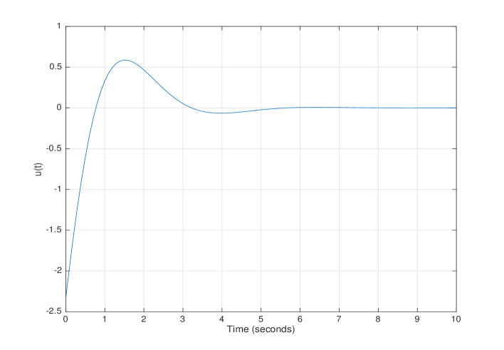
Figure 1: Precomputed Control signal for LQG control.

We use the ansatz $p_{X}\left(t\right)=K\left(t\right)\hat{X}+\varphi\left(t\right)$ where $K\left(t\right)$ is governed by the following differential matrix Riccati differential equation:

$$\dot{K}\left(t\right) =-K\left(t\right)A-A^{T}K\left(t\right)+K\left(t\right)BR^{-1}B^{T}K\left(t\right)+Q$$ (30)

$$K\left(T\right) =F$$

And $\varphi\left(t\right)$ has a dynamics driven by a backward differential equation:

$$\dot{\varphi}\left(t\right) =-\left[A-BR^{-1}B^{T}K\left(t\right)\right]^{T}\varphi\left(t\right)$$ (31)

$$\varphi\left(T\right) =0$$

This model has been simulated in MATLAB with both the Financial Toolbox (Euler-Maruyama integration method) and the Toolbox SDETool for the numerical solution of stochastic differential equations (SDEs) developed by Andrew Horchler (, and the Milstein integration method). The parameters of the quantum harmonic oscillator are $\gamma=0.1$, $\eta=0.1$, $\hbar=1$, $m=\frac{1}{2}$, and $\omega_{0}=1$ rad/seg. The cost functional is built with the matrices $R=Q=20I_{2}$  where $I_{2}$ stands for the $2\times 2$ identity matrix. The terminal time is chosen as $T=10$ sec. and the integration step was chosen as $dt=0.1$ sec.

The initial conditions for the problem were selected so as to satisfy the Heisenberg uncertainty principle,

$$\hat{X}\left(0\right) =\left(1,1\right)$$

$$\Sigma\left(0\right) =\left(\begin{array}[c]{cc}1&1\\ 1&\frac{\hbar^{2}}{2}\end{array}\right)$$

The action control $u\left(t\right)$ is precomputed according to the ansatz via the expression $-R^{-1}B^{T}\left(K\left(t\right)\hat{X}+\varphi\left(t\right)\right)$. Since the backward differential equations for $K\left(t\right)$ and $\varphi\left(t\right)$ are hard to be analytically solved we have decided on numerically solving them through the Runge-Kutta (4,5) method with integration step $dt$ and then interpolating the result with splines. The precomputed control signal is shown in Figure 1 where the action control decreases as the system gains information. The asymptotic behaviour is such that $\lim_{t\rightarrow\infty}u\left(t\right)=0$ since the uncertainty diminishes to zero as time goes to infinity.

The position and the momentum of the particle are plotted both for the uncontrolled case in Figure 2a and for the LQG control in Figure 2b.

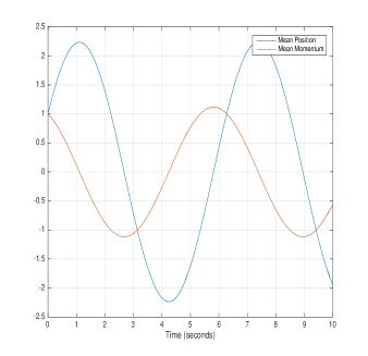
(a) Uncontrolled QHO.

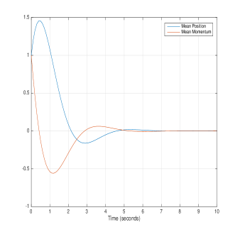
(b) Controlled QHO with a LQG controller

Figure 2: Mean position and mean momentum for the Quantum Harmonic Oscillator.

VI Conclusions

A quantum maximum principle has been addressed for
continuous-time measurements. This has been derived from the Hamilton-Jacobi-Bellman equation in the Schrödinger picture. Then the scheme has been extended to the Heisenberg picture in statistical moment coordinates. Since a stochastic Pontryagin principle requires a numerical solution to solve the equations we have derived a LQG scheme which is more suitable for control purposes.

The Pontryagin principle tapes its roots in the method of Lagrange multipliers applied in constrained optimization. A constraint on the state essentially introduces infinitely many additional constraints compared with a deterministic state constrained control problem; PMP approach allows to transform an infinite dimensional optimization problem (the search over a set of functions) into a finite dimensional optimization problem (the search over a set of parameters). In the future it should be interesting to explore QOC problems under state constraints.

Appendix A Quantum Linear Model

Let $H_{sys}$ be the free Hamiltonian of the system, and let $L_{k}$ and $S_{k}$ be bounded system operators specifying the coupling and the scattering of the system to the k-th measurement channel respectively. The operator-valued process $U\left(t\right)$ representing the joint evolution of the composite quantum system has a dynamics governed by a quantum stochastic differential equation (QSDE) of the form:

$$dU\left(t\right) =\left(-\frac{\mathbf{i}}{\hbar}\left(H_{sys}+H\left(u\right)\right)+\frac{1}{2}L^{\dagger}L\right)U\left(t\right)dt+\sum_{i=1}^{2m}L_{i}U\left(t\right)dA_{i}^{\dagger}\left(t\right)-\sum_{i=1}^{2m}L_{i}^{\dagger}U\left(t\right)dA_{i}\left(t\right)$$ (32)

$$U\left(0\right) =I$$

where $H\left(u\right)$ is the controlled Hamiltonian. Adapted process $A_{i}\left(t\right)$, $A_{i}^{\dagger}\left(t\right)$ and $Idt$ satisfy the Itô’s multiplication rule. The creation process $A_{i}^{\dagger}\left(t\right)$ and the annihilation process $A_{i}\left(t\right)$ are diffusive.

The time evolution of the operator $X\in\mathcal{A}$ is defined as the Markovian flow $j_{t}\left(X\right)=U^{\dagger}\left(t\right)\left(X\otimes I\right)U\left(t\right)$. The application of the Itô’s relations to $X\left(t\right)=j_{t}\left(X\right)$ allows us to obtain the well-known Heisenberg-Langevin equations:

$$dX_{k}\left(t\right)=\mathcal{L}_{t}\left[X_{k}\left(t\right)\right]dt+\sum_{i=1}^{d}\left[X_{k}\left(t\right),L_{i}\right]dA_{i}^{\dagger}\left(t\right)-\sum_{i=1}^{d}\left[X_{k}\left(t\right),L_{i}^{\dagger}\right]dA_{i}\left(t\right)$$ (33)

where $\mathcal{L}_{t}\left[X\right]=j_{t}\left(\mathcal{L}\left[X\right]\right)$ stands for the time evolution of the Gorini-Kossakovski-Sudarshan generator

$$\mathcal{L}\left[X\right]=\frac{1}{2}\sum_{i=1}^{d}L_{i}^{\dagger}\left[X,L_{i}\right]-\frac{1}{2}\left[X,L_{i}^{\dagger}\right]L_{i}+\frac{\mathbf{i}}{\hbar}\left[H_{sys}+H(u),X\right]$$ (34)

and is given by

$$\mathcal{L}_{t}\left[X\right]=j_{t}\left(\mathcal{L}\left[X\right]\right)=\frac{1}{2}\sum_{i=1}^{d}L_{i}^{\dagger}\left(t\right)\left[X\left(t\right),L_{i}\left(t\right)\right]-\frac{1}{2}\sum_{i=1}^{d}\left[X\left(t\right),L_{i}^{\dagger}\left(t\right)\right]L_{i}\left(t\right)+\frac{\mathbf{i}}{h}\left[H_{sys}+H\left(u\right),X\left(t\right)\right]$$ (35)

In deriving $\left(\ref{EQA401}\right)$ note that $j_{t}\left(\left[X,Y\right]\right)=\left[X\left(t\right),Y\left(t\right)\right]$ and that $j_{t}\left(XY\right)=X\left(t\right)Y\left(t\right)$, for arbitrary operators $X,Y\in\mathcal{A}$.

A.1 Evolution of the Operator $\mathcal{L}_{t}\left[X_{k}\right]$

A.1.1 System Hamiltonian

For the system Hamiltonian $H_{sys}=\mathbb{X}^{\intercal}\left(R\otimes I\right)\mathbb{X}$ we first derive $\left[H_{sys},X_{k}\right]=H_{sys}X_{k}-X_{k}H_{sys}$. The identities $\left[X_{k},X_{i}\right]=\hbar S_{k,i}$ and $X_{j}X_{k}=\left[X_{j},X_{k}\right]+X_{k}X_{j}$ allows us to write the following relations:

$$H_{sys}X_{k} =\frac{1}{2}\sum_{i,j}r_{i,j}X_{i}X_{j}X_{k}=\frac{1}{2}\sum_{i,j=1}^{2m}r_{i,j}\left(\hbar S_{k,i}S_{j,k}X_{i}+X_{i}X_{k}X_{j}\right)$$

$$X_{k}H_{sys} =\frac{1}{2}\sum_{i,j}r_{i,j}X_{k}X_{i}X_{j}=\frac{1}{2}\sum_{i,j=1}^{2m}r_{i,j}\left(\hbar S_{k,i}S_{k,i}X_{j}+X_{i}X_{k}X_{j}\right)$$

and then

$$\left[H_{sys},X_{k}\right]=\frac{1}{2}\sum_{i,j=1}^{2m}r_{i,j}\hbar S_{k,i}\left(S_{k,i}S_{j,k}X_{i}-S_{k,i}S_{k,i}X_{j}\right)$$ (36)

On the other hand

$$\sum_{i,j=1}^{2m}r_{i,j}S_{k,i}X_{j}=\hbar\left(\begin{array}[c]{ccccc}S_{k,1}I&S_{k,2}I&S_{k,3}I&\cdots&S_{k,2m}I\end{array}\right)\left(R\otimes I\right)\mathbb{X}$$ (37)

Similarly,

$$\mathbf{i}\hbar\sum_{i,j=1}^{2m}r_{i,j}S_{j,k}X_{i}=\mathbb{X}^{\intercal}\left(R\otimes I\right)\left(\begin{array}[c]{c}S_{1,k}I\\ S_{2,k}I\\ \vdots\\ S_{2m,k}I\end{array}\right)=$$ (42)

$$=-\hbar\left(\begin{array}[c]{ccccc}S_{k,1}I&S_{k,2}I&S_{k,3}I&\cdots&S_{k,m}I\end{array}\right)\left(R^{T}\otimes I\right)\mathbb{X}$$ (44)

For the sake of simplicity we use the notation $\left[H_{sys},\mathbb{X}\right]$ to refer to the stacking of operators $\left[H_{sys},X_{k}\right]$. According to $\left(\ref{EQA404}\right)$ and $\left(\ref{EQA405}\right)$ it is straightforward that

$$\left[H_{sys},\mathbb{X}\right]=-\frac{1}{2}\hbar\left(\mathbb{S}\left(R+R^{T}\right)\otimes I\right)\mathbb{X}$$ (45)

A.1.2 Controlled Hamiltonian

We define the controlled Hamiltonian as

$$H\left(u\right)=\frac{1}{2}\left(u^{T}\left(K^{T}+K^{\dagger}\right)\otimes I\right)\mathbb{X}$$ (46)

or more explicitly

$$H\left(u\right)=\frac{1}{2}\sum_{i=1}^{2m}\left(u^{T}\left(K^{T}+K^{\dagger}\right)\mathbf{e}_{i}\right)X_{i}$$ (47)

For each $X_{k}\in\mathcal{A}$ in $\mathbb{X}$ we compute the bracket $\left[H\left(u\right),X_{k}\right]$. Since $H\left(u\right)$ is a linear combination of operators $X_{i}$, and recalling that $\left[X_{i},X_{k}\right]=\hbar S_{i,k}$, we can write

$$\left[H\left(u\right),X_{k}\right]-\frac{1}{2}\sum_{i=1}^{2m}\hbar S_{k,i}e_{i}^{T}\left(K+K^{\ast}\right)uI$$

and in compact form

$$\left[H\left(u\right),\mathbb{X}\right]=-\frac{\hbar}{2}\left(\mathbb{S}\left(K+K^{\ast}\right)\otimes I\right)\left(u\otimes I\right)$$

Defining $B=\frac{1}{2}\left(\mathbb{S}\left(K+K^{\ast}\right)\otimes I\right)$ and $v\left(t\right)=\left(u\left(t\right)\otimes I\right)$, we get the control term $Bv\left(t\right)$ in the SDE.

A.1.3 Coupling terms

The coupling operator $L_{i}$ for the i-th measurement channel depends on the state $\mathbb{X}$:

$$L_{i}=\sum_{i=1}^{2m}\Gamma_{il}X_{l}$$

We begin writing the brackets

$$\left[X_{k},L_{i}\right]=\sum_{j=1}^{2m}\Gamma_{i,j}\left[X_{k},X_{j}\right]=\hbar\sum_{j=1}^{2m}\Gamma_{i,j}S_{k,j}I$$ (48)

$$\left[L_{i}^{\dagger},X_{k}\right]=\sum_{j=1}^{2m}\Gamma_{i,j}^{\ast}\left[X_{j}^{\dagger},X_{k}\right]$$ (49)

The bracket $\left[X_{j}^{\dagger},X_{k}\right]$ in $\left(\ref{EQA506}\right)$ is a little more involved and deserves more attention. First of all,

$$\left[X_{j}^{\dagger},X_{k}\right]=\left\{\begin{array}[c]{cc}\left[X_{j+m},X_{k}\right]=\hbar S_{j+m,k}&\text{, if }j\leq m\\ \left[X_{j}^{\dagger},X_{k}\right]=\left[\left(X_{j-m}^{\dagger}\right)^{\dagger},X_{k}\right]=\hbar S_{j-m,k}&\text{, if }j>m\end{array}\right.$$ (50)

Secondly, from $\left(\ref{EQA508}\right)$ we observe that the effect of $\left[X_{j}^{\dagger},X_{k}\right]$ is to exchange the row blocks in the partitioned matrix $\mathbb{S}$, i.e. $\left[X_{j}^{\dagger},X_{k}\right]=\hbar\left(\mathbb{JS}\right)_{j,k}I$. By exploiting the identities $\left(\mathbb{JS}\right)^{T}=\mathbb{S}^{T}\mathbb{J}^{T}=-\mathbb{SJ}$, the bracket is conveniently written as $\left[X_{j}^{\dagger},X_{k}\right]=-\hbar\left(\mathbb{SJ}\right)_{j,k}I$.

Introducing this information into $\left(\ref{EQA506}\right)$ and $\left(\ref{EQA507}\right)$ yields:

$$\sum_{i=1}^{d}L_{i}^{\dagger}\left[X_{k},L_{i}\right]=\hbar\sum_{i=1}^{d}\sum_{j,l=1}^{2m}\Gamma_{i,j}\Gamma_{i,l}^{\ast}S_{k,j}X_{l}^{\dagger}$$ (51)

$$\sum_{i=1}^{d}\left[L_{i}^{\dagger},X_{k}\right]L_{i}=-\hbar\sum_{i=1}^{d}\sum_{j,l=1}^{2m}\Gamma_{i,j}^{\ast}\Gamma_{i,l}\left(\mathbb{SJ}\right)_{j,k}X_{l}$$ (52)

Finally,

$$\sum_{i=1}^{d}L_{i}^{\dagger}\left[X_{k},L_{i}\right]=\hbar\sum_{i=1}^{d}\sum_{j,l=1}^{2m}S_{k,j}\Gamma_{j,i}^{T}\Gamma_{i,l}^{\ast}X_{l}^{\dagger}=\hbar\sum_{l=1}^{2m}\left(\mathbb{S}\Gamma^{T}\Gamma^{\ast}\right)_{kl}X_{l}^{\dagger}$$ (53)

$$\sum_{i=1}^{d}\left[L_{i}^{\dagger},X_{k}\right]L_{i}=-\hbar\sum_{l=1}^{2m}\left(\mathbb{SJ}\Gamma^{\dagger}\Gamma\right)_{kl}X_{l}$$ (54)

and in compact form

$$\frac{1}{2}\left(\sum_{i=1}^{d}L_{i}^{\dagger}\left[X,L_{i}\right]-\left[X,L_{i}^{\dagger}\right]L_{i}\right)=\frac{\hbar}{2}\mathbb{S}\left(\left(\Gamma^{T}\Gamma^{\ast}\mathbb{J}+\mathbb{J}\Gamma^{\dagger}\Gamma\right)\otimes I\right)\mathbb{X}$$ (55)

From $\left(\ref{EQA513}\right)$ and $\left(\ref{EQA514}\right)$ we define

$$A=\frac{\hbar}{2}\left(\mathbb{S}\left(R+R^{T}+\left(\Gamma^{T}\Gamma^{\ast}\mathbb{J}+\mathbb{J}\Gamma^{\dagger}\Gamma\right)\right)\otimes I\right)$$

which corresponds to the term $A\mathbb{X}$ in the SDE.

A.1.4 Terms of Uncertainty

The uncertainty terms in $\left(\ref{EQA502}\right)$ can be computed by resorting to $\left(\ref{EQA506}\right)$, $\left(\ref{EQA507}\right)$ and $\left(\ref{EQA508}\right)$:

$$\sum_{i=1}^{d}\left[X_{k}\left(t\right),L_{i}\right]dA_{i}^{\dagger}\left(t\right)=\sum_{i=1}^{d}\sum_{j=1}^{2m}\Gamma_{i,j}\left[X_{k},X_{j}\right]dA_{i}^{\dagger}\left(t\right)=\hbar\sum_{i=1}^{d}\sum_{j=1}^{2m}S_{k,j}\left(\Gamma^{T}\right)_{j,i}dA_{i}^{\dagger}\left(t\right)$$

$$\sum_{i=1}^{d}\left[L_{i}^{\dagger},X_{k}\right]dA_{i}\left(t\right)=\hbar\sum_{i=1}^{d}\sum_{j=1}^{2m}\left(\mathbb{JS}\right)_{k,j}\Gamma_{j,i}^{\dagger}dA_{i}\left(t\right)$$ (56)

Calling $\mathbb{A}$ and $\mathbb{A}^{\dagger}$to the stacking of operators $A_{i}$ and $A_{i}^{\dagger}$, the noise increment in the state equation is given by

$$dW\left(t\right)=\hbar\left(\mathbb{S}\Gamma^{T}\mathbb{J}\otimes I\right)d\mathbb{A}^{\dagger}\left(t\right)+\hbar\left(\mathbb{JS}\Gamma\otimes I\right)d\mathbb{A}\left(t\right)$$

A.1.5 Output Equation

The field quadrature for the i-th output channel is given by $A_{i}+A_{i}^{\dagger}$. The output in the channel $i$ is considered as the weak measurement $Y_{i}\left(t\right)=U^{\dagger}\left(t\right)\left(\left(A_{i}+A_{i}^{\dagger}\right)\otimes I\right)U\left(t\right)$. The application of the Itô formula to $Y_{i}\left(t\right)$ yields:

$$dY_{i}\left(t\right)=\left(L_{i}+L_{i}^{\dagger}\right)dt+dA_{i}+dA_{i}^{\dagger}$$

which can be compactly written as

$$dY\left(t\right)=\left(\left(\Gamma+\Gamma^{\ast}\right)\otimes I\right)\mathbb{X}dt+\left(d\mathbb{A}\left(t\right)+d\mathbb{A}^{\dagger}\left(t\right)\right)$$

Note that

$$L_{i}+L_{i}^{\dagger} =\sum_{l=1}^{2m}\Gamma_{il}X_{l}+\Gamma_{il}^{\ast}X_{l}^{\dagger}=$$

$$=\sum_{l=1}^{m}\Gamma_{il}X_{l}+\sum_{l=m+1}^{2m}\Gamma_{il}^{\ast}X_{l}+$$

$$+\sum_{l=m+1}^{2m}\Gamma_{il}X_{l}+\sum_{l=1}^{m}\Gamma_{il}^{\ast}X_{l}$$

Data Availability

The data that support the findings of this study are available from the corresponding author upon reasonable request.

References

• (1) H. Wiseman and G. Milburn, Quantum Measurement and Control.   Cambridge University Press, 2010.
• (2) S. J. Glaser, U. Boscain, T. Calarco, C. P. Koch, W. Köckenberger, R. Kosloff, I. Kuprov, B. Luy, S. Schirmer, T. Schulte-Herbrüggen, D. Sugny, and F. K. Wilhelm, “Training Schrödinger’s cat: quantum optimal control,” The European Physical Journal D, vol. 69, no. 12, p. 279, 2015.
• (3) M. Shapiro and P. Brumer, Quantum Control of Molecular Processes.   Wiley Interscience, 2012.
• (4) N. Khaneja, T. Reiss, B. Luy, and S. J. Glaser, “Optimal control of spin dynamics in the presence of relaxation,” Journal of Magnetic Resonance, vol. 162, no. 2, pp. 311 – 319, 2003.
• (5) Q.-M. Chen, R.-B. Wu, T.-M. Zhang, and H. Rabitz, “Near-time-optimal control for quantum systems,” Phys. Rev. A, vol. 92, p. 063415, Dec 2015.
• (6) J. A. Budagosky, D. V. Khomitsky, E. Y. Sherman, and A. Castro, “Shaped electric fields for fast optimal manipulation of electron spin and position in a double quantum dot,” Phys. Rev. B, vol. 93, p. 035423, Jan 2016.
• (7) P. A. Golovinskii, “Pontryagin principle of maximum for the quantum problem of speed,” Automation and Remote Control, vol. 68, no. 4, pp. 610–618, 2007.
• (8) K. Jacobs and D.  A. Steck, “A Straightforward Introduction to Continuous Quantum Measurement,” Contemp.Phys, vol. 47, pp. 279, 2006.
• (9) A.  A. Clerk, M.  H. Devoret, S.  M. Girvin, F. Marquardt, and R.  J. Schoelkopf, “Introduction to quantum noise, measurement, and amplification,” Rev. Mod. Phys, vol. 82, pp. 1155, 2010.
• (10) K. Jacobs and A. Shabani, “Quantum feedback control: how to use verification theorems and viscosity solutions to find optimal protocols,” Contemp.Phys, vol. 49, pp. 435, 2008.
• (11) H. Yuan, C. P. Koch, P. Salamon, and D. J. Tannor, “Controllability on relaxation-free subspaces: On the relationship between adiabatic population transfer and optimal control,” Phys. Rev. A, vol. 85, p. 033417, Mar 2012.
• (12) K. H. Hoffmann, P. Salamon, Y. Rezek, and R. Kosloff, “Time-optimal controls for frictionless cooling in harmonic traps,” EPL (Europhysics Letters), vol. 96, no. 6, p. 60015, 2011.
• (13) P. Salamon, K. H. Hoffmann, Y. Rezek, and R. Kosloff, “Maximum work in minimum time from a conservative quantum system,” Phys. Chem. Chem. Phys., vol. 11, pp. 1027–1032, 2009.
• (14) D.  Stefanatos, H. Schaettler, J.S.  Li, "Minimum-time frictionless atom cooling in harmonic traps", SIAM Journal on Control and Optimization vol. 49 no. 6, p. 2440-2462, 2011.
• (15) D.  Stefanatos, "Minimum-time transitions between thermal equilibrium states of the quantum parametric oscillator", IEEE Transactions on Automatic Control vol. 62, p. 4290 – 4297, 2017.
• (16) D.  Stefanatos, "Minimum-Time Transitions between Thermal and Fixed Average Energy States of the Quantum Parametric Oscillator", SIAM Journal on Control and Optimization vol. 55 no. 3, p. 1429-1451, 2017.
• (17) Y. Rezek, P. Salamon, K. H. Hoffmann, and R. Kosloff, “The quantum refrigerator: The quest for absolute zero,” EPL (Europhysics Letters), vol. 85, no. 3, p. 30008.
• (18) H. Jirari and W. Pötz, “Quantum optimal control theory and dynamic coupling in the spin-boson model,” Phys. Rev. A, vol. 74, p. 022306, Aug 2006.
• (19) V. Mukherjee, A. Carlini, A. Mari, T. Caneva, S. Montangero, T. Calarco, R. Fazio, and V. Giovannetti, “Speeding up and slowing down the relaxation of a qubit by optimal control,” Phys. Rev. A, vol. 88, p. 062326, Dec 2013.
• (20) M. Lapert, Y. Zhang, M. Braun, S. J. Glaser, and D. Sugny, “Singular extremals for the time-optimal control of dissipative spin $\frac{1}{2}$ particles,” Phys. Rev. Lett., vol. 104, p. 083001, Feb 2010.
• (21) N. Khaneja, R. Brockett, and S. J. Glaser, “Time optimal control in spin systems,” Phys. Rev. A, vol. 63, p. 032308, Feb 2001.
• (22) A. Garon, S. J. Glaser, and D. Sugny, “Time-optimal control of su(2) quantum operations,” Phys. Rev. A, vol. 88, p. 043422, Oct 2013.
• (23) D.  D’Alessandro and M.  Dahleh, "Optimal control of two-level quantum systems", IEEE Transactions on Automatic Control vol. 46, p. 866-876, 2001.
• (24) U.  Boscain, G.  Charlot, J.P.  Gauthier, S.  Guérin, H.R.  Jauslin, "Optimal control in laser-induced population transfer for two-and three-level quantum systems", Journal of Mathematical Physics vol. 43 no. 5, p. 2107-2132, 2002.
• (25) U.  Boscain, P.  Mason, "Time minimal trajectories for a spin $1/2$ particle in a magnetic field", Journal of Mathematical Physics vol. 47 no. 6, 062101, 2006.
• (26) D.  Stefanatos, J.S.  Li, "Constrained minimum-energy optimal control of the dissipative Bloch equations", Systems & Control Letters vol. 59 no. 10, p. 601-607, 2010.
• (27) B.  Bonnard, M.  Chyba, D.  Sugny, "Time-minimal control of dissipative two-level quantum systems: The generic case", IEEE Transactions on Automatic control vol. 54 no. 11, p. 2598-2610, 2009.
• (28) D. Stefanatos, “Optimal shortcuts to adiabaticity for a quantum piston,” Automatica, vol. 49, no. 10, pp. 3079 – 3083, 2013.
• (29) R.  Roloff, M.  Wenin, W.  Pötz, "Optimal Control for Open Quantum Systems: Qubits and Quantum Gates" ,J. Comput. Theor. Nanosci., vol. 49, no. 6, pp. 1837, 2019.
• (30) D.  Sugny and C.  Kontz, "Optimal control of a three-level quantum system by laser fields plus von Neumann measurements", Phys. Rev. A, vol. 77, 063420 2008.
• (31) Y.  Wang, R.  Wu, X.  Chen, Y.  Ge, J.  Shi, H.  Rabitz, F.  Shuang, "Quantum state transformation by optimal projective measurements" Journal of Mathematical Chemistry, vol. 49, Issue 2, pp 507–519, 2011.
• (32) D. J. Egger and F. K. Wilhelm, "Optimal control of a quantum measurement", Phys. Rev. A vol. 90, 052331, 2014.
• (33) V. Belavkin, "Measurement, filtering and control in quantum open dynamical systems", Rep. Math. Phys, vol. 43, p.405-425, 1999.
• (34) I. R.  Petersen, "Quantum Linear Systems Theory", eprint arXiv:1603.04950, March 2016
• (35) D.  Dong, I. R.  Petersen, "Quantum control theory and applications: A survey", IEEE Tran. Control Theory & Applications, vol. 4, no. 12, p. 2651-2671, 2010.
• (36) J. Zhang, Y.X..  Liu, R.B. Wu, K.  Jacobs, F.  Nori, "Quantum feedback: theory, experiments, and applications", Physics Reports vol. 679, p.1-60 2017.
• (37) J. V. Neumann, Mathematical Foundations of Quantum Mechanics, ser. Investigations in physics.   Princeton University Press, 1955.
• (38) V. Belavkin and M. Guta, Quantum Stochastics and Information: Statistics, Filtering and Control.   World Scientific Publishing Company, 2008.
• (39) J. Yong and X. Zhou, Stochastic Controls: Hamiltonian Systems and HJB Equations, ser. Stochastic Modelling and Applied Probability.   Springer New York, 2012.
• (40) L. Bouten, R. van Handel, and M. R. James, “An introduction to quantum filtering,” SIAM J. Control and Optimization, vol. 46, no. 6, pp. 2199–2241, 2007.
• (41) C. Gardiner and P. Zoller, Quantum Noise: A Handbook of Markovian and Non-Markovian Quantum Stochastic Methods with Applications to Quantum Optics, ser. Springer Series in Synergetics.   Springer, 2004.
• (42) K. Parthasarathy, An Introduction to Quantum Stochastic Calculus, ser. Modern Birkhäuser Classics.   Springer Basel, 2012.
• (43) S. C. Edwards and V. P. Belavkin, “Optimal Quantum Filtering and Quantum Feedback Control,” eprint arXiv:quant-ph/0506018, June 2005.
• (44) B. Aliprantis, I. Dobbs, Optimisation and Stability Theory for Economic Analysis.   Cambridge University Press, 1990.
• (45) C. D. Aliprantis and C. Kim, Infinite Dimensional Analysis.   Springer Verlag, Berlin, 2006.
• (46) J. Yong and X. Y. Zhou, Stochastic Controls: Hamiltonian Systems and HJB Equations.   Springer-Verlag New York, 1999.
• (47) A. C. Doherty and K. Jacobs, “Feedback Control of Quantum Systems using Continuous State Estimation,“ Phys. Rev. A vol. 60, no. 4, pp. 2700 – 2711, 1999.